1. Introduction
Human activities in the offshore region are continually increasing due to oil and gas exploration. Adverse conditions can often occur due to environmental disasters during offshore operations. Predicting wave characteristics is a crucial prerequisite for offshore oil and gas development (
Figure 1), considering the safety of lives and the avoidance of economic damage. Wave height and period are typically significantly increased by the wind associated with storms passing across the ocean’s surface. Weather forecasting departments usually predict wind forces rather than wave periods and heights. There are several empirical approaches for estimating wave height and wave period from wind force [
1,
2,
3,
4,
5]. Estimating wave height and period is inherently inaccurate and random, making it difficult to simulate using deterministic equations [
6]. The numerical approach for calculating wave height and period is a difficult and complex procedure that, despite substantial breakthroughs in computational tools, produces solutions that are neither dependable nor consistently applicable. Machine learning methods are perfect for modeling inputs with corresponding outputs since they do not necessitate an understanding of the underlying physical mechanism [
7].
Several studies have been performed using artificial neural networks (ANN) to measure important wave heights and mean-zero-up-crossing wave period history for different locations in the seas. These parameters were predicted three, six, twelve, and twenty-four hours in advance using two different neural network methods [
8,
9,
10]. The time series of these wave parameters has been investigated using simulations in Portugal’s western coast area. Time series with wave height have been disintegrated into multi-resolution time series using wavelet transformation hybridized with ANN and wavelet transformation [
11,
12]. As the input of the ANN, the multi-resolution time series has been used to predict the important wave height at an unlike multi-step lead time near Mangalore, India’s west coast. Mandal et al. [
13] expected wave heights from observed ocean waves off the west coast of India, Marmugao. To predict wave height, recurrent neural networks with a resilient propagation (Rprop) update algorithm have been implemented.
The time series of wave height and mean-zero-up crossing wave period were simulated using data from the local wind. The application of various types of machine learning models [
14,
15,
16,
17] was performed to improve the accuracy of the prediction. The authors [
18] used ANN to estimate wave height from wind force at 10 chosen locations in the Baltic Sea. The WAM4 wave model was used to figure out the time series for the waves that had been forecasted in the past. There were two different techniques, Feed-forward Back-propagation (FFBP) and Radial Basis Function (RBF), used to develop a machine learning system for predicting wave heights at a particular coastal point in deeper offshore areas [
19,
20,
21]. Data on wave height, average wave period, and wind speed were obtained from remotely sensed satellite data on India’s west coast. Tsai et al. [
22] employed the ANN with a back-propagation algorithm to estimate wave height and cycle from wind input based on the wind-wave relationship [
23]. Time records of waves at either station may be predicted based on data from the neighboring station. Several deterministic neural network models have been developed by Deo et al. [
24] to predict wave height and wave periods from generated wind speed. However, the model can offer adequate results in deep water and open areas, and the prediction periods are extensive.
This research uses wind force/metocean data to correctly predict wave height and wave period. Critical comparisons are performed for the current investigation to provide more accurate findings in predicting the wave parameters using three machine learning algorithms: ANN (Artificial Neural Network), SVM (Support Vector Machine), and RF (Random Forest).
The main contributions of the paper are (i) performing the experiments on the data sets obtained on the east coast of Malaysia and (ii) understanding the best predictive models for future prediction.
We arrange the remaining parts of the manuscript as follows. First, we explain the data collection procedures, the three regressor models, and performance metrics used for the comparison among the models in
Section 2. Then, we show the experimental results and discuss the findings in
Section 3. Finally,
Section 4 contains a concise conclusion.
2. Materials and Methods
In this section, first, the data collection procedure is described, followed by the regression methods, and finally the evaluation metrics are described.
2.1. Data Collection
On a 2° × 2° grid in South China, environmental data are collected along Malaysia’s east coast, including the basins of Sabah (longitude 114.39° E, latitude 5.83° N) and Sarawak (longitude 111.82° E, latitude 5.15° N) (
Figure 2). The Malaysian Meteorological Service and Fugro OCEANOR provided the data that was acquired from satellite altimetry [
25,
26] using oceanographic SEAWATCH meteorological (metocean) buoys and sensors, calibrated and corrected by Fugro OCEANOR [
27].
The summary of common statistical values of the collected data is given in
Table 1.
There are 1460 data samples and three features: wind speed (m/s), wave height (m), and wave period (s).
2.2. Methods
There are a lot of algorithms [
28,
29,
30,
31,
32,
33] that can be used for regression analysis. In this study, three well-known and commonly used regression algorithms (ANN, SVM, and RF) were chosen to predict wave height and period from wind force. The wind force is employed as an input for training the network, while the wave height and period are used as outputs. Before discussing the details of each method,
Table 2 shows the advantages and disadvantages of each method [
34]:
The ANN algorithm is the most frequently utilized algorithm in such problems. The difference between the state-of-the-art ANN algorithm and two commonly used algorithms, SVM and RF, is then determined. Note that ANN is a parametric regression algorithm while SVM and RF are nonparametric regression algorithms. However, because the data set is small enough, it is not possible to employ advanced deep learning techniques (such as convolutional neural networks or recurrent neural networks).
2.2.1. Artificial Neural Network (ANN)
Inspiring by biological neurons, the researchers created artificial neurons [
35]. It is possible to create a network of artificial neurons to predict the desired functions (i.e., the target variables).
The basic idea behind a single artificial neuron is that it takes an input function
I, which is a product of weight vectors with the sample input vector, and feeds it into an activation function
g to produce an output (
Figure 3). Generally, the usual practice is to create a network of neurons based on many layers: input layers, hidden layers, and output layers. The input layers basically consist of one or more neurons based on the supplied inputs (for the present study, only one input is used), then there can be one or more hidden layers (only one hidden layer is used), and finally, there can be one output layer consisting of the expected outputs (
Figure 4). The general trend is to use a back-propagation algorithm to update the weights involved in each connection between neurons so that it is possible to minimize the errors of regression between true output and the predicted output.
The hyperbolic tangent function, is used as the activation function.
The steps of the Python implementation are described in Algorithm 1.
| Algorithm 1 The Python implementation of the ANN algorithm |
Input: Data set containing features and target
Output: Prediction of ANN for the given data set
1. Read the data set using the Python read_excel function;
2. Extract features and target variables;
3. Scale the features and target using the MinMaxScaler function;
4. Split the data set into training and test parts using the train_test_split function;
5. Choose the best hyperparameter using the GridSearchCV function;
6. Derive the MLPRegressor using the above results;
7. Predict using the obtained regressor and calculate the performance metrics on the test data set; |
2.2.2. Support Vector Machine (SVM)
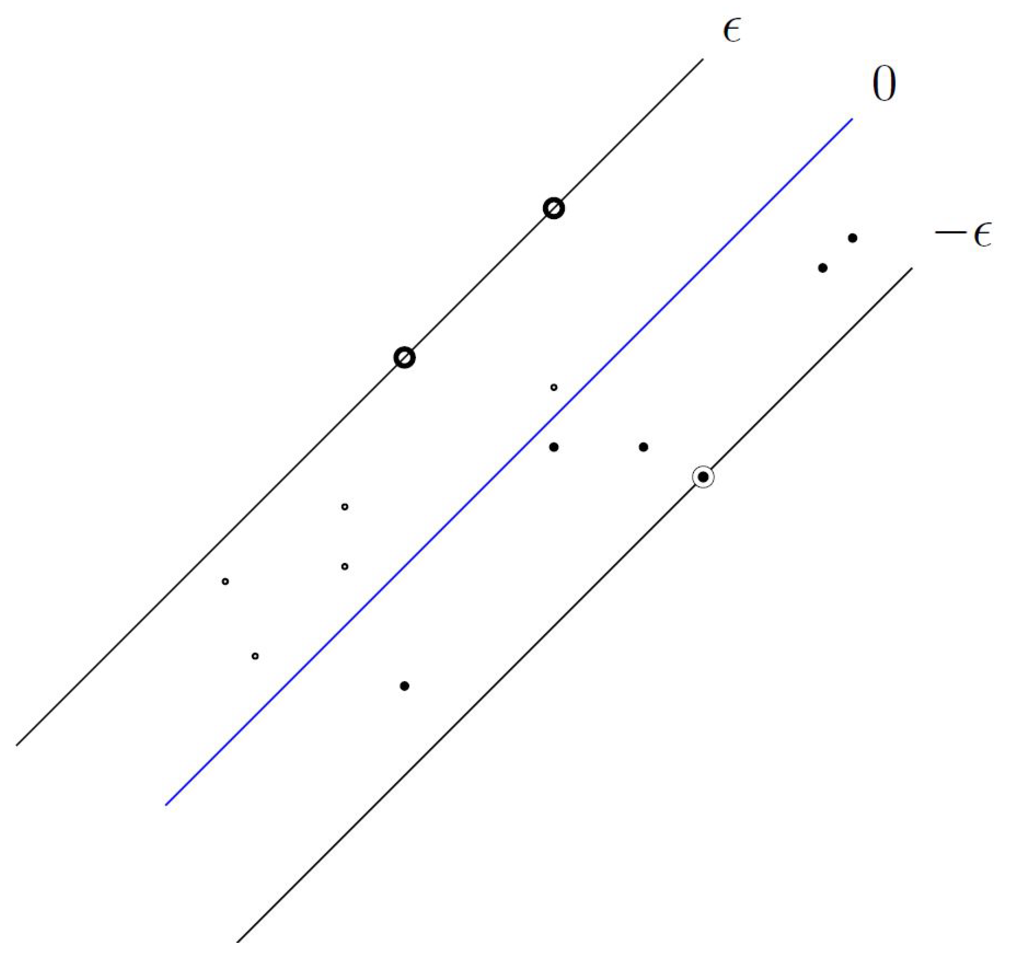
The basic idea behind regression using SVM (i.e., also popularly known as Support Vector Regression) is that given input examples
, where
X denotes the example space (e.g.,
for our problem), a function
is obtained that has at most
deviation from the actual outputs oi for all the input examples (
Figure 5) [
36].
Generally, it is easy to describe the case of linear functions [
37]
f,
, with
where denotes the dot product in X. Furthermore, it is possible to rewrite this problem as a convex optimization problem:
minimize
subject to
The steps of the Python implementation are described in Algorithm 2.
| Algorithm 2 The python implementation of the SVR algorithm |
Input: Data set containing features and target
Output: Prediction of SVR for the given data set
1. Read the data set using the Python read_excel function;
2. Extract features and target variables;
3. Scale the features and target using the StandardScaler function;
4. Split the data set into training and test parts using the train_test_split function;
5. Choose the best hyperparameter using the GridSearchCV function;
6. Derive the SVR using the above results;
7. Predict using the obtained regressor and calculate the performance metrics on the test data set; |
2.2.3. Random Forest (RF)
A decision tree has been widely used from the very beginning of machine learning research to find the best hypothesis as the classifier and regressor. A decision tree is a tree-like structure where a sequence of actions is taken from the root to the leaf nodes based on the values of each decision node in the concerned path. A sample decision tree is depicted in
Figure 6, where the course of action of playing outside is taken based on the value of whether it is training outside or not.
There are a number of different variants of decision tree algorithms, from ID3 [
38], C4.5 [
39], and CART [
40] to ensembles of decision trees (e.g., Random Forest [
28])) that have been proposed to improve the accuracy of the classifiers and regressors. For a single decision tree construction, the most widely used splitting criteria, “Gini index” or “Entropy”, can be mathematically stated as follows [
32,
38,
39,
40,
41]:
where T is the data set and is the set of labels in the data set T. In addition, represents the number of samples and represents the number of samples with the label t.
A Random Forest (RF) is an ensemble of decision tree models such that each tree in the ensemble is built based on the bootstrap samples of the training data set. Furthermore, during the construction of the decision trees, the random forest selects only a subset of the features at each split point. In this way, the constructed decision trees are more different from each other to reduce the correlation among them and to have a better prediction. In contrast to the single decision tree (CART), random forests do not use any pruning of the tree.
Like any ensemble algorithm, the random forest also takes the average among all decision tree regressors to produce the final predictions (
Figure 7).
The steps of the Python implementation are described in Algorithm 3.
| Algorithm 3 The Python implementation of the RF algorithm |
Input: Data set containing features and target
Output: Prediction of RF for the given data set
1. Read the data set using the Python read_excel function;
2. Extract features and target variables;
3. Scale the features and target using the MinMaxScaler function;
4. Split the data set into training and test parts using the train_test_split function;
5. Choose the best hyperparameter using the GridSearchCV function;
6. Derive the RandomForestRegressor using the above results;
7. Predict using the obtained regressor and calculate the performance metrics on the test data set; |
2.3. Performance Metrics
Four performance metrics [
42] have been used for the comparison of the results.
Mean squared error ()
Root mean squared error ()
Mean absolute error ()
Coefficient of determination ()
For each sample, the error (
) is the difference between actual output (
) and predicted output (
). The average of the squares of the error (
) is the
. The average is taken by dividing the summation of the square of all the errors by the total number of samples (
n).
Root mean squared error (
) is the square root of the average difference in squared error between actual output (
) and predicted output (
). It is the most commonly used metric.
Mean absolute error (
) is the average absolute difference of error between actual output (
) and predicted output (
). It is the most commonly used metric. The advantage of
is that it is softer to outliers. The reason is that it does not have any square term associated with the equation, therefore the penalty for the outlier points is not that much compared to
and
where there are heavy penalties imposed by the square term.
The coefficient of determination or
explains the degree to which the independent variables explain the variation of the output variable. It is a measure of how well new samples can be predicted by the model through the proportion of explained variance. If
is the true value of the
i-th sample and
is the corresponding output or predicted value, the estimated
can be calculated as:
where
.
3. Results and Discussion
The experiments have been executed based on the available field data from the east coast of Malaysia, which consists of 1460 samples, one input variable, wind speed (m/s), and one target variable, either wave height (m) or wave period (s). The regression results are compared among the three regressors (ANN, SVM, and RF). The Python programming environment (version ) with scikit-learn (version ) is used for the implementation.
Initially, the ANN regressor is trained using the training data and then the accuracy is validated using the testing data. The network is chosen with one hidden layer of 4 neurons, and each neuron uses the hyperbolic tangent function. The weight of the ANN is optimized using “lbfgs” in the family of quasi-Newton methods. Furthermore, the SVM regressor is trained using the same training data and validated using the same testing data as mentioned above. For SVM, the standard radial basis function (RBF) is used as the kernel function. Finally, the RF regressor is trained and validated in a similar fashion. For RF, 400 trees are used for the number of trees, 3 is used for the maximum depth of the tree, and samples are used for the training of each decision tree in the ensembles. Each regressor is compared by the state-of-the-art performance metrics.
3.1. Cross Validation Results
It is a common practice to keep a part of the available data for testing and the remaining part for training. However, the model evaluation is particularly dependent on specific pairs of (training and testing) fractions, and the result can be overfitting. To overcome this problem, cross validation [
43] is used to test the model’s fitness to predict new data that was not used to train the model and how it can generalize to unknown data.
There are many variants of cross-validation. The standard method is to use k-fold cross-validation. In general, the procedure is to use k rounds in cross-validation. It splits the data into k subsets. In a single round, it completes the analysis on one subset (the training set), and then validates the performance on the remaining subsets (the validation set). In the next round, another subset is chosen for training and the remaining is chosen for validation. To reduce variability, these steps are repeated k times for k subsets so that each subset is selected for training. Finally, an average among the k validation results is reported as the fitness of the model’s predictive performance.
Nevertheless, it is common practice to repeat the k-fold cross-validation process multiple times and report the average performance among all folds and all repeats. This approach is called repeated k-fold cross-validation.
The average and standard deviation of the regression performance of wave height were determined using 10-fold cross validation that was done for three methods as presented in
Table 3. The four-performance metrics are reported in the same way as in the preceding section.
It is clearly evident that the method of ANN has a minimum average value of mean absolute error, mean square error, and root mean square error. Besides, it has the maximum average value of the coefficient of determination. As a result, this approach performs best for predicting wave height.
Similar findings for wave period have been presented in
Table 4 using 10-fold cross validation that has been done for the consecutive three methods.
It is apparent that the RF approach has the lowest mean absolute error, mean square error, and root mean square error. Furthermore, it has the maximum value of the coefficient of correlation. As a result, this approach is the most accurate for predicting wave periods.
is close to 1, which indicates that regression predictions perfectly fit the data. However, in our case, the experimental results show the lower value of due to the inconsistencies in the collected data set.
3.2. Graphical Representation of a Sample Training and Testing Results
To illustrate the model’s performance graphically, one sample is chosen randomly as the pair of (training, testing), where the training is 80% and testing is 20% of the data. In
Table 5, the results for both training and testing data are shown in the case of the wave height regression problem. It is evident that the mean squared error, mean absolute error, and root mean squared errors are the smallest for RF compared to others in the training data. However, these metrics are the smallest for ANN compared to others in the testing data. Furthermore, the coefficient of correlation (
) is largest for RF compared to others in the training data, but it is largest for ANN compared to others in the testing data. As a result, the ANN approach is superior at predicting wave height in the future.
The regression results of ANN, SVM, and RF for wave height are depicted in
Figure 8.
Figure 8a shows the ANN regression findings for wave height. The black dots are actual testing data, and the green dots are the predicted values. It is clear that the predicted values follow the pattern of the actual testing data. Nevertheless, the regression results for the SVM regressor are shown in
Figure 8b. The black dots are actual testing data, and the blue dots are the predicted values. It is clear that the predicted values follow the pattern of the actual testing data.
The regression results of wave height based on the RF regressor are presented in
Figure 8c. The black dots are actual testing data, and the orange dots are the predicted values. It is clear that the predicted values follow the pattern of the actual testing data. The pattern is not as smooth as SVM or ANN because RF is not a single decision tree method; rather it is an ensemble method that works by taking the average of different decision trees’ predictions.
In addition, in the case of wave period,
Table 6 shows the findings for both training and testing data. It is evident that the mean squared error, mean absolute error, and root mean squared error is the smallest for RF compared to others in both training and testing data. Nevertheless, the coefficient of determination (
) is the largest for RF compared to others in both training and testing data. Therefore, for future prediction of wave period, the RF method is best.
The regression results of ANN, SVM, and RF for wave period are depicted in
Figure 9. For ANN, in
Figure 9a, the actual testing data is shown in black dots and the predicted values are shown in green dots. It is clear that the predicted values follow the pattern of the actual testing data for ANN. For SVM, in
Figure 9b, the actual testing data are represented by black dots, while the actual predicted values are represented by blue dots. It is clear that the predicted values follow the pattern of the actual testing data for SVM.
Finally, for RF, the real testing data is represented in black dots, whereas the actual predicted values are shown in orange dots in
Figure 9c. It is clear that the predicted values follow the pattern of the actual testing data for RF. The pattern is not as smooth as SVM or ANN because RF is not a single decision tree method; rather it is an ensemble method that works by taking the average of different decision trees’ predictions.
3.3. Comparison with Standard Non-Parametric Kernel Regression
The non-parametric method of kernel regression (KR) in statistics is used to calculate the conditional expectation of a random variable. The goal is to find a non-linear relationship between two random variables,
I and
O [
44]. The problem under consideration can be modeled using a standard non-parametric regression problem. As an example,
I can be wind speed and
O can be wave height. In
Table 7, the previous results are compared with the results of KR for the same sample.
It is clear that KR results are not far from those of the SVM, ANN, or RF. In fact, ANN produces the best results in the case of wave height prediction.
3.4. Overall Discussion
The goal of this study is to understand the best predictive model among ANN, SVM, and RF for the prediction of wave height and period from the wind speed. A detailed experiments are performed in terms of cross-validation and sample training and testing results. The summary of this result is given in the
Table 8.
It is evident from
Table 8 that the Random Forest (RF) method is truly performing well across two prediction problems. It is the second best for the prediction of wave height and the best for predicting wave period. Nevertheless, it has the advantage of being a non-parametric method. Moreover, the underlying tree structure has the advantages of interpretability and usage. However, to be specific, RF performs best for the prediction of wave period while ANN performs best for the prediction of wave height.
4. Conclusions
This study carried out three different and well-known machine learning algorithms for the prediction of offshore waves. These approaches are used to predict the wave height and wave period from the given wind forces. Multiple accuracy ranges are obtained in terms of the mean absolute error, mean square error, root mean square error, and coefficient of determination. Overall, these performance measures show average behavior. However, it is possible to compare the three employed methods and analyze the results. The regression analysis in the random forest performs best for the prediction of wave period, and the artificial neural network performs best for the prediction of wave height. Furthermore, it was compared with the standard non-parametric kernel regression and found to have a similar result.
In situations when a traditional analysis would be challenging, these machine learning techniques can produce very quick and reasonable predictions. These studies can benefit the community as a measurement of safety and precaution in the critical marine environment.
In this regard, there are numerous potential future research directions. One disadvantage of using such metocean data is the existence of discrepancies. Future work should incorporate advanced algorithms in addition to the aforementioned models to address such inconsistencies. Additionally, more machine learning techniques should be used to find the ideal answer for this specific prediction problem. The time dependence of the metocean data, which can be examined using time series analysis tools, is another interesting subject of research.
Author Contributions
Conceptualization, all authors; methodology, all authors; software, M.A.; validation, M.A.; formal analysis, all authors; investigation, all authors; resources, all authors; data curation, M.A.U.; writing, all authors; visualization, all authors; supervision, all authors.; project administration, M.A.U.; funding acquisition, M.A. All authors have read and agreed to the published version of the manuscript.
Funding
This research received no external funding.
Institutional Review Board Statement
Not applicable.
Informed Consent Statement
Not applicable.
Data Availability Statement
It is available with a justifiable and reasonable request.
Acknowledgments
The authors are grateful to Jouf University for their assistance with this research. Moreover, the authors would like to express their gratitude to all of the volunteers and anonymous reviewers for their suggestions.
Conflicts of Interest
The authors declare no conflict of interest.
References
- Krogstad, H.; Barstow, S. Satellite wave measurements for coastal engineering applications. Coast. Eng. 1999, 37, 283–307. [Google Scholar] [CrossRef]
- Tolman, H.; Alves, J.; Chao, Y. Operational Forecasting of Wind-Generated Waves by Hurricane Isabel at NCEP*. Weather Forecast. 2005, 20, 544–557. [Google Scholar] [CrossRef]
- Tolman, H.; Balasubramaniyan, B.; Burroughs, L.; Chalikov, D.; Chao, Y.; Chen, H.; Gerald, V.M. Development and Implementation of Wind-Generated Ocean Surface Wave Modelsat NCEP. Weather Forecast. 2002, 17, 311–333. [Google Scholar] [CrossRef]
- Günther, H.; Rosenthal, W.; Stawarz, M.; Carretero, J.; Gomez, M.; Lozano, I.; Serrano, O.; Reistad, M. The wave climate of the Northeast Atlantic over the period 1955–1994: The WASA wave hindcast. Glob. Atmos. Ocean Syst. 1998, 6, 121–163. [Google Scholar]
- Muzathik, A.M.; Nik, W.B.W.; Samo, K.; Ibrahim, M.Z. Ocean Wave Measurement and Wave Climate Prediction of Peninsular Malaysia. J. Phys. Sci. 2011, 22, 79–94. [Google Scholar]
- Setiawan, I.; Yuni, S.M.; Miftahuddin, M.; Ilhamsyah, Y. Prediction of the height and period of sea waves in the coastal waters of Meulaboh, Aceh Province, Indonesia. J. Physics: Conf. Ser. 2021, 1882, 012013. [Google Scholar] [CrossRef]
- Wang, J.; Wang, Y.; Yang, J. Forecasting of Significant Wave Height Based on Gated Recurrent Unit Network in the Taiwan Strait and Its Adjacent Waters. Water 2021, 13, 86. [Google Scholar] [CrossRef]
- Makarynskyy, O.; Makarynska, D.; Kuhn, M.; Featherstone, W. Predicting sea level variations with artificial neural networks at Hillarys Boat Harbour, Western Australia. Estuar. Coast. Shelf Sci. 2004, 61, 351–360. [Google Scholar] [CrossRef]
- Makarynskyy, O.; Pires-Silva, A.; Makarynska, D.; Ventura-Soares, C. Artificial neural networks in wave predictions at the west coast of Portugal. Comput. Geosci. 2005, 31, 415–424. [Google Scholar] [CrossRef]
- Kambekar, A.; Deo, M. Real Time Wave Forecasting Using Wind Time History and Genetic Programming. Int. J. Ocean Clim. Syst. 2014, 5, 249–260. [Google Scholar] [CrossRef]
- Deka, P.C.; Prahlada, R. Discrete wavelet neural network approach in significant wave height forecasting for multistep lead time. Ocean Eng. 2012, 43, 32–42. [Google Scholar] [CrossRef]
- Wu, M.; Stefanakos, C.; Gao, Z.; Haver, S. Prediction of short-term wind and wave conditions for marine operations using a multi-step-ahead decomposition-ANFIS model and quantification of its uncertainty. Ocean Eng. 2019, 188, 106300. [Google Scholar] [CrossRef]
- Mandal, S.; Prabaharan, N. Ocean wave forecasting using recurrent neural networks. Ocean Eng. 2006, 33, 1401–1410. [Google Scholar] [CrossRef]
- Wei, C.C. Wind Features Extracted from Weather Simulations for Wind-Wave Prediction Using High-Resolution Neural Networks. J. Mar. Sci. Eng. 2021, 9, 1257. [Google Scholar] [CrossRef]
- Hu, H.; Westhuysen, A.; Chu, P.; Fujisaki-Manome, A. Predicting Lake Erie wave heights using XGBoost and LSTM. Ocean Model. 2021, 164, 101832. [Google Scholar] [CrossRef]
- Wei, C.C.; Cheng, J.Y. Nearshore two-step typhoon wind-wave prediction using deep recurrent neural networks. J. Hydroinform. 2019, 22, 346–367. [Google Scholar] [CrossRef]
- Juliani, V.; Adytia, D.; Adiwijaya. Wave Height Prediction based on Wind Information by using General Regression Neural Network, study case in Jakarta Bay. In Proceedings of the 2020 8th International Conference on Information and Communication Technology (ICoICT), Yogyakarta, Indonesia, 24–26 June 2020; pp. 1–5. [Google Scholar] [CrossRef]
- Paplińska-Swerpel, B. Application of Neural Networks to the Prediction of Significant Wave Height at Selected Locations on the Baltic Sea. Arch. Hydroeng. Environ. Mech. 2006, 53, 183–201. [Google Scholar]
- Kalra, R.; Deo, M.; Kumar, R.; Agarwal, V. Artificial neural network to translate offshore satellite wave data to coastal locations. Ocean Eng. 2005, 32, 1917–1932. [Google Scholar] [CrossRef]
- Uddin, M.A.; Jameel, M.; Abdul Razak, H.; Islam, A.B.M. Response Prediction of Offshore Floating Structure Using Artificial Neural Network. Adv. Sci. Lett. 2012, 14, 186–189. [Google Scholar] [CrossRef]
- Ellenson, A.; Özkan Haller, H. Predicting Large Ocean Wave Events Characterized by Bi-Modal Energy Spectra in the Presence of a Low-Level SoutherlyWind Feature. Weather Forecast. 2018, 33. [Google Scholar] [CrossRef]
- Tsai, C.P.; Lin, C.; Shen, J.N. Neural network for wave forecasting among multi-stations. Ocean Eng. 2002, 29, 1683–1695. [Google Scholar] [CrossRef]
- Londhe, S.; Panchang, V. One-Day Wave Forecasts Based on Artificial Neural Networks. J. Atmos. Ocean. Technol. 2006, 23, 1593–1603. [Google Scholar] [CrossRef]
- Deo, M.; Jha, A.; Chaphekar, A.; Ravikant, K. Neural networks for wave forecasting. Ocean Eng. 2001, 28, 889–898. [Google Scholar] [CrossRef]
- Yaakob, O.; Zainudin, N.; Samian, Y.; Malik, A.M.A.; Palaraman, R.A. Developing Malaysian Ocean Wave Database Using Satellite. In Proceedings of the 25th Asian Conference on Remote Sensing, Chiang Mai, Thailand, 22–26 November 2004. [Google Scholar]
- Yaakob, O.; Hashim, F.; Omar, K.; Md Din, A.H.; Koh, K. Satellite-based wave data and wave energy resource assessment for South China Sea. Renew. Energy 2015, 88, 359–371. [Google Scholar] [CrossRef]
- FUGRO. Fugro Metocean Services. 2022. Available online: https://www.fugro.com/media-centre/news/fulldetails/2009/10/05/20-years-and-100-countries—worldwaves-a-success-story (accessed on 5 August 2022).
- Breiman, L. Random Forests. Mach. Learn. 2001, 45, 5–32. [Google Scholar] [CrossRef]
- Azad, M. Knowledge Representation Using Decision Trees Constructed Based on Binary Splits. KSII Trans. Internet Inf. Syst. 2020, 14, 4007–4024. [Google Scholar] [CrossRef]
- Azad, M.; Chikalov, I.; Moshkov, M. Decision Trees for Knowledge Representation. In Proceedings of the 28th International Workshop on Concurrency, Specification and Programming, CS&P 2019, Olsztyn, Poland, 24–26 September 2019; Ropiak, K., Polkowski, L., Artiemjew, P., Eds.; CEUR-WS.org—CEUR Workshop Proceedings: Aachen, Germany, 2019; Volume 2571. [Google Scholar]
- Azad, M.; Chikalov, I.; Hussain, S.; Moshkov, M. Multi-Pruning of Decision Trees for Knowledge Representation and Classification. In Proceedings of the 3rd IAPR Asian Conference on Pattern Recognition, ACPR 2015, Kuala Lumpur, Malaysia, 3–6 November 2015; pp. 604–608. [Google Scholar]
- Alsolami, F.; Azad, M.; Chikalov, I.; Moshkov, M. Decision and Inhibitory Trees and Rules for Decision Tables with Many-Valued Decisions;Intelligent Systems Reference Library; Springer: Berlin/Heidelberg, Germany, 2020; Volume 156. [Google Scholar]
- Azad, M.; Moshkov, M. A Bi-criteria Optimization Model for Adjusting the Decision Tree Parameters. Kuwait J. Sci. 2022, 49, 1–14. [Google Scholar] [CrossRef]
- Juárez-Orozco, L.; Martinez Manzanera, O.; Nesterov, S.; Kajander, S.; Knuuti, J. The machine learning horizon in cardiac hybrid imaging. Eur. J. Hybrid Imaging 2018, 2, 1–15. [Google Scholar] [CrossRef]
- McCulloch, W.S.; Pitts, W. A Logical Calculus of the Ideas Immanent in Nervous Activity. In Neurocomputing: Foundations of Research; MIT Press: Cambridge, MA, USA, 1988; pp. 15–27. [Google Scholar]
- Boser, B.; Guyon, I.; Vapnik, V. A Training Algorithm for Optimal Margin Classifier. In Proceedings of the Fifth Annual Workshop on Computational Learning Theory, Pittsburgh, PA, USA, 27–29 July 1992; Volume 5. [Google Scholar] [CrossRef]
- Smola, A.; Schölkopf, B. A tutorial on support vector regression. Stat. Comput. 2004, 14, 199–222. [Google Scholar] [CrossRef]
- Quinlan, J.R. Induction of decision trees. Mach. Learn. 1986, 1, 81–106. [Google Scholar] [CrossRef]
- Quinlan, J.R. C4. 5: Programs for Machine Learning; Morgan Kaufmann: Burlington, MA, USA, 1992. [Google Scholar]
- Breiman, L.; Friedman, J.H.; Olshen, R.A.; Stone, C.J. Classification and Regression Trees; Wadsworth and Brooks: Monterey, CA, USA, 1984. [Google Scholar]
- Azad, M.; Chikalov, I.; Hussain, S.; Moshkov, M.; Zielosko, B. Decision Trees with Hypotheses (To Appear); Synthesis Lectures on Intelligent Technologies; Springer: Berlin/Heidelberg, Germany, 2022. [Google Scholar]
- Botchkarev, A. A New Typology Design of Performance Metrics to Measure Errors in Machine Learning Regression Algorithms. Interdiscip. J. Inf. Knowl. Manag. 2019, 14, 045–076. [Google Scholar] [CrossRef]
- Hastie, T.; Tibshirani, R.; Friedman, J. The Elements of Statistical Learning; Springer Series in Statistics; Springer Inc.: New York, NY, USA, 2001. [Google Scholar]
- Wikipedia Contributors. Kernel Regression—Wikipedia, the Free Encyclopedia. 2022. Available online: https://en.wikipedia.org/w/index.php?title=Kernel_regression&oldid=1099742212 (accessed on 7 July 2022).
| Publisher’s Note: MDPI stays neutral with regard to jurisdictional claims in published maps and institutional affiliations. |
© 2022 by the authors. Licensee MDPI, Basel, Switzerland. This article is an open access article distributed under the terms and conditions of the Creative Commons Attribution (CC BY) license (https://creativecommons.org/licenses/by/4.0/).


