Simultaneous Estimation of Vehicle Mass and Unknown Road Roughness Based on Adaptive Extended Kalman Filtering of Suspension Systems

Abstract

This study presents a vehicle mass estimation system based on adaptive extended Kalman filtering with unknown input (AEKF-UI) estimation of vehicle suspension systems. The suggested real-time methodology is based on the explicit correlation between road roughness and suspension system. Because the road roughness input influences the suspension system, AEKF-UI with a forgetting factor is proposed to simultaneously estimate the time-varying parameter (vehicle mass) of vehicle suspension systems and road roughness using an unknown input estimator. However, a constant forgetting factor does not adaptively weigh the covariance of all the states, and optimal filtering cannot be ensured. To resolve this problem, we present an adaptive forgetting factor technique employed to track time-varying parameters and unknown inputs. Simulation studies demonstrate that the proposed algorithm can simultaneously estimate the vehicle mass variation and unknown road roughness input. The feasibility and effectiveness of the proposed estimation algorithm were verified through laboratory-level experiments.

1. Introduction

In recent years, accurate monitoring of vehicle state information has attracted increasing attention because it is critical for high-precision control of future vehicles such as autonomous as well as conventional vehicles. In particular, vehicle mass is one of the essential parameters in many automotive control systems, and its accuracy directly affects control robustness. For example, the automotive control system requiring accurate vehicle mass includes the active safety system such as collision avoidance [1], active suspension control [2], an electronic stability program [3], etc. The real vehicle mass can change significantly depending on the carried loads of vehicles and to be estimated for control purposes. However, it is challenging to directly measure it by using typical mechanical sensors. Therefore, several studies have attempted to indirectly estimate vehicle mass. These studies have focused on using the longitudinal dynamics of a vehicle to estimate the vehicle mass. Most current techniques for estimating vehicle mass rely on longitudinal and lateral vehicle dynamic models [4,5,6,7,8,9,10,11,12].

Lin et al. [4] established a mass estimation method that considers systematic errors in longitudinal vehicle dynamics. Huh et al. [5] proposed an integrated mass-estimation algorithm based on longitudinal, lateral, and vertical suspension dynamics. Min Zhao et al. [6] presented a vehicle mass dynamics based on a vehicle longitudinal dynamics model that considers the effects of the braking and cornering joint estimation method based on the vehicle longitudinal dynamics model, considering the effects of braking and cornering. Reina et al. [7] proposed an extended Kalman filter to estimate vehicle mass based on the lateral vehicle dynamic model and several sensors such as gyroscope and accelerometers.

In addition, some researchers have studied simultaneous estimation of vehicle mass and road slope. The observer-based parameter estimation scheme for road gradient and vehicle mass had been proposed based on the knowledge of longitudinal dynamics and driving information [8,9,10,11]. Zhang et al. [12] present a dual-level reinforcement estimator to estimate the total mass and road slope of electric mining haul trucks (EMHTs). However, the estimation based on longitudinal dynamics has some technical limitations. It requires the estimation of many systems information (i.e., vehicle speed, engine torque, gear ratio, brake signal, etc.) and unknown disturbance inputs (i.e., road load). Those can inherently generate a lot of noise and affect the accuracy of the estimation results. For these reasons, there were only studies on the simultaneous estimation of vehicle mass and road slope.

In this study, we explore a vehicle mass estimation system based on vertical vehicle dynamics instead of longitudinal vehicle dynamics because suspension systems governed by vertical vehicle dynamics suffer from only single unknown disturbance input (i.e., road roughness). In contrast, the longitudinal vehicle dynamics suffer from several system information and unknown disturbance inputs called road loads such as gradient due to gravitation force, aerodynamic drag, rolling resistance, etc. Some research for vehicle mass estimation has been proposed based on a vertical dynamic system. Jordan et al. [13] proposed the vehicle mass estimator using a multi-model filter. The proposed method is derived by using a vertical dynamic system to reduce the effort of a calibrated referenced dual Kalman filter for the estimation of road irregularities and vehicle mass under a vertical dynamic system. Boada et al. [14] had proposed the dual Kalman filter which requires suspension deflection sensors and an accelerometer. However, this method just parallel estimates vehicle mass and road roughness. Because the estimation performance for vehicle mass can be affected by road roughness (frequently referred to as road profile), a simultaneous estimation method for vehicle mass and road roughness should be developed.

In fact, the measurement of road roughness is challenging owing to the expensive sensors [15]. As a result, an alternative method of road roughness estimation had been proposed based on a suspension system. The Youla–Kucera (YK) parametric observer, which takes advantage of adaptive control law, such as Q-parameterization or YK parameterization, was proposed and used to successfully estimate the road profile [16]. In addition, an H∞ observer was proposed to estimate the road profile using onboard accelerometers. The goal was to minimize the effect of sensor noise on the estimation error using the H∞ framework [17]. However, these approaches are complicated, and vehicle mass estimation performance has not been validated experimentally. Kang et al. applied the Kalman filter algorithm to estimate road roughness and evaluated its performance using an in-vehicle test [18]. Kim et al. estimated the road roughness and state information of a suspension control system based on a Kalman filter with an unknown input (KF-UI) [19,20]. In addition, the Kalman filter with the forgetting factor method had been applied to several systems such as a lithium-ion battery to consider the variation of system model parameters [21]. However, the estimation accuracy of the KF-UI cannot be guaranteed under both unknown input and model parameter variations.

Therefore, the objective of this study is to resolve the aforementioned issues in the estimation of time-varying vehicle mass and unknown road roughness, and we employed a vehicle suspension model (vertical dynamics) and an adaptive extended Kalman filter with unknown input combined with forgetting factor update algorithm, as shown in Figure 1. The paper is organized as follows. The quarter-car suspension model is described in Section 2. Thereafter, the real-time estimation of vehicle mass based on vertical vehicle dynamics (vehicle suspension system) and the Kalman filter (AEKF-UI) is presented in Section 3. Finally, simulations and experimental validation are presented in Section 4 and Section 5.

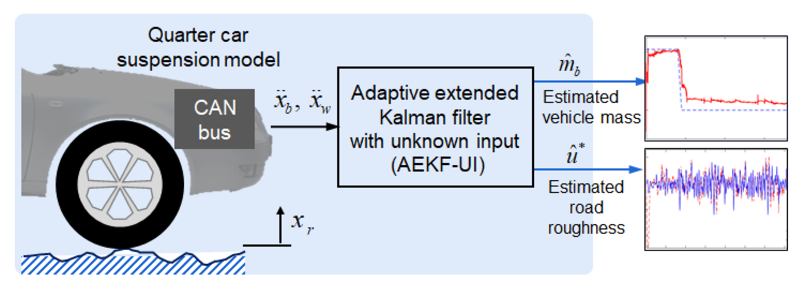
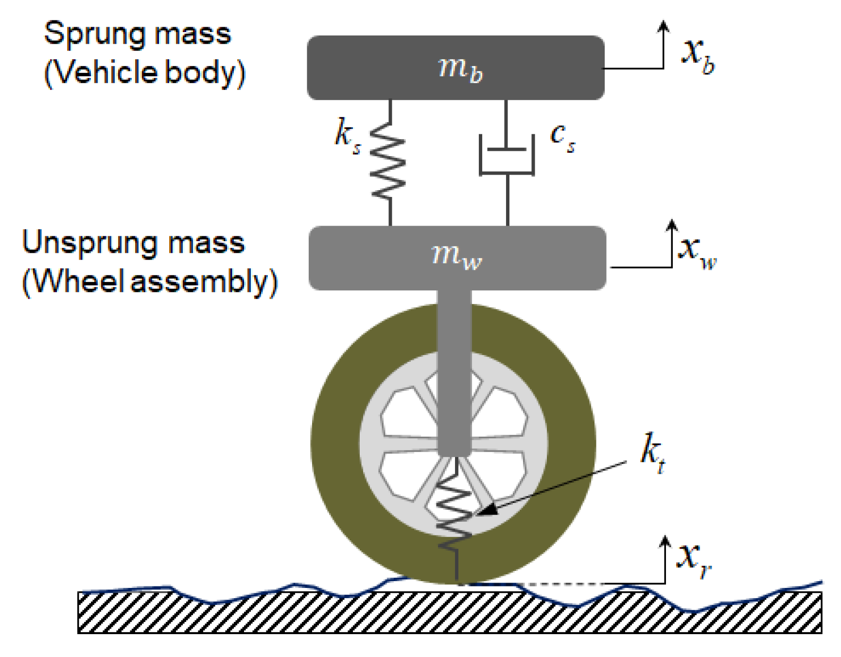
2. Quarter-Car Suspension Model

Various vehicle models have been developed for different purposes. The suitability of each model depends on the performance evaluation criteria. The quarter-car suspension model consists of two degrees of freedom, with the primary masses consisting of the sprung mass (vehicle mass) and the unsprung mass (mass of one wheel, tire, and shock absorber), whereas the linear sprung (tire stiffness $k_t$) associated with the unsprung mass models the tire, as shown in Figure 2. Although the linear quarter-car model ignores the more complex linkage effects, it simplifies complex real-world suspension systems and is thus easier to research and widely used [22,23]. Therefore, a simple suspension system is beneficial for embedded systems. Therefore, a simple suspension mechanism is advantageous for embedded devices. Many researchers have studied and integrated embedded systems using these benefits for better controlling or analyzing vehicle suspension systems. The same passive quarter-car suspension model was utilized in this work to estimate vehicle mass and road roughness ($x_r$) as an unknown input.

The governing equations of a quarter-car suspension model are derived as follows:

$$\begin{gathered} m_b{\ddot{x}}_b+c_s\left({\dot{x}}_b-{\dot{x}}_w\right)+k_s\left(x_b-x_w\right)=0 \\ {m}_w{\ddot{x}}_w+c_s\left({\dot{x}}_w-{\dot{x}}_b\right)+k_s\left(x_w-x_b\right)+k_t{x}_w=k_t{x}_r \end{gathered}$$

(1)

Equation (1) is converted into a nonlinear state equation with an unknown time-varying parameter (i.e., car mass) as the state variable of the quarter-suspension system, and the time-varying parameter is expanded into a state vector as follows:

$$\begin{gathered} \begin{array}{l}\mathrm{x}={\left[\begin{array}{ccccc}{x}_b& {\dot{x}}_b& x_w& {\dot{x}}_w& m_b\end{array}\right]}^T={\left[\begin{array}{ccccc}{x}_1& x_2& x_3& x_4& x_5\end{array}\right]}^T\\ u^{*}=x_r\end{array} \\ \dot{x}=\left[\begin{array}{c}{\dot{x}}_1\\ {\dot{x}}_2\\ {\dot{x}}_3\\ {\dot{x}}_4\\ {\dot{x}}_5\end{array}\right]=\left[\begin{array}{c}{x}_2\\ \frac{k_s\left(x_3-x_1\right)+c_s(x_4-x_2)}{x_5}\\ x_4\\ \frac{k_s\left(x_1-x_3\right)+c_s\left(x_2-x_4\right)+k_t\left(x_r-x_3\right)}{m_w}\\ 0\end{array}\right] \end{gathered}$$

(2)

$$y=\left[\begin{array}{c}{\ddot{x}}_b\\ {\ddot{x}}_w\end{array}\right]=\left[\begin{array}{c}\frac{k_s\left(x_3-x_1\right)+c_s(x_4-x_2)}{x_5}\\ \frac{k_s\left(x_1-x_3\right)+c_s\left(x_2-x_4\right)+k_t\left(x_r-x_3\right)}{m_w}\end{array}\right]$$

(3)

where the sprung and unsprung mass displacements are $x_b$ and $x_w$, respectively, the road roughness (profile elevation) $x_r$ is an unknown input for the system, the sprung and unsprung masses are $x_5$ and $x_w$, respectively. Note that the extended Kalman filter for nonlinear systems should be designed because the two state variables ($x_5$ and $x_3$) in Equation (3) are coupled. The suspension model was described as a hierarchical sprung with stiffness and a linear damper with a damping constant. A pneumatic tire was modeled as stiffness. The vehicle mass is then unknown and can be modeled as a state variable of the random-walk model. This state–space model can be represented by the following equations:

$$\begin{array}{l}\dot{x}=f(x,u^{*},w)\\ y=h(x,u^{*},v)\end{array}$$

(4)

where $x$ is the state variable vector defined in Equation (3), w is the process noise, v is the measurement noise, f is the system function, u* is the unknown input for the system, h is the output function, $y$ is the measurable output vector, and ${\ddot{x}}_b$ and ${\ddot{x}}_w$ are the sprung and unsprung mass acceleration, respectively. The acceleration signals (${\ddot{x}}_b$ and ${\ddot{x}}_w$) can be obtained from the CAN (Controller Area Network) bus.

3. Adaptive Extended Kalman Filter with Unknown Input Estimation

3.1. Overview

In Kalman filtering theory, nonlinear systems can be modeled and identified using an extended Kalman filter (EKF) [24,25]. EKF-UI was extended with a forgetting factor (i.e., AEKF-UI). Compared with EKF-UI, AEKF-UI can estimate the time-varying system parameters. However, constant forgetting cannot guarantee optimal performance. To enhance the tracking ability and robustness to noise, an adaptive fading Kalman filter was developed by [26]. In this study, this technique was employed to track time-varying parameters, such as sprung mass. As a result, under the present state error model, the outdated data may have an impact on AEKF-UI. Errors in the state assumption are caused by the filter presumption’s reliance on old data. The derivation of the AEKF-UI can be expressed as follows:

$${\dot{x}}_k=\frac{x_k-x_{k-1}}{\Delta t}\Rightarrow x_k={\dot{x}}_k\Delta t+x_{k-1}=x_{k-1}+f(x,u^{*},w)\Delta t$$

(5)

where Δt is the time step and k and k − 1 indicate the time instants at t = kΔt and t = (k − 1)Δt, respectively. Replacing Equation (2) with Equation (5) yields. The global discrete equation for Equation (6) is as follows:

$$\{\begin{array}{l}{x}_k=f_{k-1}(x_{k-1},u_{k-1}^{*},w_{k-1})\\ y_k=h_k(x_k,u_k^{*},v_k)\end{array}$$

(6)

where $x_k\in {ℝ}^{n\times 1}$ denotes the system state vector, $y_k\in {ℝ}^{m\times 1}$ denotes the measured variable vector, $u_k^{*}\in {ℝ}^{1\times 1}$ is the unknown input vector, $w_k\in {ℝ}^{n\times 1}$ is the process noise, and $v_k\in {ℝ}^{m\times 1}$ is the measurement noise vector. It is assumed that the measured sprung mass and the unsprung mass acceleration are sampled at the exact time instant $k\cdot T(k=0,1,2$⋯).

$$E[w_k{w}_j^T]=Q_k\cdot {\delta }_{kj}$$

(7)

$$E[v_k{v}_j^T]=R_k\cdot {\delta }_{kj}$$

(8)

where ${\delta }_k$ and $E[\cdot ]$ denote the Kronecker delta and expected value operator, respectively. $\left\{w_k\right\}$ and $\left\{v_k\right\}$ denote sequences of uncorrelated Gaussian random vectors with zero mean, and $Q_k$ and $R_{k }$represent covariance matrices. The AEKF-UI algorithm can then be summarized as follows:

• Initialization of the filter at k = 0

$$\{\begin{array}{l}{\widehat{x}}_0^{+}=E[x_0]\\ {\widehat{u}}_0^{*}=E[u_0^{*}]\\ P_0^{+}=E[(x_0-{\widehat{x}}_0^{+}){(x_0-{\widehat{x}}_0^{+})}^T]\\ S_0=E[(u_0^{*}-{\widehat{u}}_0^{*}){(u_0^{*}-{\widehat{u}}_0^{*})}^T]\end{array}$$

(9)

• Prediction stage

$$\begin{gathered} A_{k-1}={\frac{\partial f_{k-1}}{\partial x}|}_{{\widehat{x}}_{k-1}^{+}}=\left[\begin{array}{ccccc}0& 1& 0& 0& 0\\ \frac{-k_s}{x_5}& \frac{-c_s}{x_5}& \frac{k_s}{x_5}& \frac{c_s}{x_5}& 0\\ 0& 0& 1& 0& 0\\ \frac{k_s}{m_w}& \frac{c_s}{m_w}& \frac{-k_s-k_t}{m_w}& \frac{-c_s}{m_w}& 0\\ 0& 0& 0& 0& 0\end{array}\right] \\ {\widehat{x}}_k^{-}=f_{k-1}({\widehat{x}}_{k-1},u_{k-1}^{*},0) \end{gathered}$$

(10)

$$P_k^{-}={\lambda }_{k-1}{A}_{k-1}{P}_{k-1}^{+}{A}_{k-1}^T+Q_{k-1},\hspace{0.17em}{\lambda }_k\ge 1$$

(11)

The a priori estimate is denoted by the superscript −. The prediction stage then updates the state estimate and estimation error covariance.

• Unknown input estimation

$$H_k={\frac{\partial h_k}{\partial x}|}_{{\widehat{x}}_k^{-}},D_k^{*}={\frac{\partial h_k}{\partial u^{*}}|}_{{\widehat{u}}_k^{*}}H=\left[\begin{array}{ccccc}\frac{-k_s}{x_5}& \frac{-c_s}{x_5}& \frac{k_s}{x_5}& \frac{c_s}{x_5}& 0\\ \frac{k_s}{m_w}& \frac{c_s}{m_w}& \frac{-k_s-k_t}{m_w}& \frac{-c_s}{m_w}& 0\end{array}\right]$$

(12)

$$D^{*}={\left[\begin{array}{cc}0& \frac{k_t}{m_w}\end{array}\right]}^T$$

(13)

$$\begin{array}{l}{K}_k=P_k^{-}{H}_k^T{(H_k{P}_k^{-}{H}_k^T+R_k)}^{-1}\\ S_k={[D_k^{*T}{R}_k^{-1}(I-H_k{K}_k)D_k^{*}]}^{-1}\\ {\widehat{u}}_k^{*}=S_k{D}_k^{*T}{R}_k^{-1}(I-H_k{K}_k)\\ \hspace{1em}\hspace{1em}\times [y_k-h({\widehat{x}}_k^{-},{\widehat{u}}_{k-1}^{*})+D^{*}{\widehat{u}}_{k-1}^{*}]\end{array}$$

(14)

Equation (12) represents a partial derivation matrix $h_k$ and Equation (14) represents the Kalman gain and unknown input estimation. The superscript “+” denotes a posteriori estimate.

• Correction stage

$$\begin{array}{l}{\widehat{x}}_k^{+}={\widehat{x}}_k^{-}+K_k[y_k-h({\widehat{x}}_k^{-},{\widehat{u}}_{k-1}^{*})]\\ P_k^{+}=[I+K_k{D}_k^{*}{S}_k{D}_k^{*T}{R}_k^{-1}{H}_k]\cdot (I-K_k{H}_k)P_k^{-}\end{array}$$

(15)

Finally, the measurement of the state estimate and estimation-error covariance are updated using Equation (15). From Equations (14) and (15), the values of time-varying unknown input (road roughness) and vehicle mass are updated. The choice of forgetting factors determines the performance of AEKF-UI; therefore, the core problem is the generation of optimal forgetting factors.

$$z_k=y_k-h({\widehat{x}}_k^{-},{\widehat{u}}_{k-1}^{*})$$

(16)

$$C_{0,k}=E[z_k{z}_k^T]=H_k{P}_k^{-}{H}_k^T+R_k$$

(17)

Residual $Z_k$ is the white Gaussian noise sequence. An arbitrary gain $K_k$ in (14) is derived from the following covariance of the residual. To determine the optimal Kalman gain, the auto-covariance of the residual is first formulated as follows:

$$\begin{array}{l}{C}_j(k)=E[z_{k+j}{z}_k^T]\\ \hspace{1em}\hspace{1em} =H_{k+j}{A}_{k+j,k+j-1}\\ \hspace{1em}\hspace{1em}\hspace{1em}\times [I-K_{k+j-1}{H}_{k+j-1}]\cdots A_{k+2,k+1}\\ \hspace{1em}\hspace{1em}\hspace{1em}\times [I-K_{k+1}{H}_{k+1}]A_{k+1,k}\\ \hspace{1em}\hspace{1em}\hspace{1em}\times [P_k^{-}{H}_k^T-K_k{C}_{0,k}]\hspace{1em}\forall j=1,2,3,\cdots \end{array}$$

(18)

When Equations (14) and (17) are substituted into (18), $C_{j,i}$ should be zero, implying that the sequence of residuals is uncorrelated. However, in a practical situation, the real covariance of the residual $C_{0,i}$ is different from the theoretical value obtained from Equations (14) to (17) because of the error in the model parameters and noise covariance. Typically, innovation covariance is equal to $C_{0,i}$ when the dynamic equation is exact. However, an exact dynamic equation of a nonlinear stochastic system is not available. Therefore, the estimation error and predicted error covariance may increase owing to the effect of unknown information. Thus, $C_{j,i}$.. may not be zero, and the forgetting factor should be chosen such that the last term of $C_{j,i}$ in Equation (18) for all j = 1, 2, 3, … can be zero.

$$P_k^{-}{H}_k^T-K_k{C}_{0,k}=0$$

(19)

If Equation (19) holds, then the Kalman gain $K_{k }$ is optimal. This condition forms the basis of adaptive filtering algorithms. The term $C_{0,i}$ in Equation (19) is computed not from Equations (11)–(15) and (17) but from the measured data, $T_{k }$ and$g_{\lambda ,k}$ are defined as follows:

$$T_k=P_k^{-}{H}_k^T-K_k{C}_{0,k}$$

(20)

$$g_{\lambda ,k}=\frac{1}{2}{\displaystyle \sum _{i=1}^n{\displaystyle \sum _{j=1}^m{T}_{ij,k}^2}}$$

(21)

The optimality of the Kalman filter can be determined using Equation (21), and $T_{ij,k}^2$ is the (i,j) element $T_k$. A smaller $g_k$ implies that the Kalman gain becomes more optimal. Hence, the forgetting factor (${\lambda }_k$) should be selected to minimize $g_k$.

3.2. Forgetting Factor Update

To optimally select the forgetting factor to minimize $g_k$, we introduced the adaptive rule called p-adaptation. The constant forgetting factor is optimally updated to both identify and track a time-varying parameter based on the following equation:

$${\lambda }_k^{l+1}={\lambda }_k^l+\phi \frac{\partial g_{\lambda ,k}^l}{\partial {\lambda }_k^l}\hspace{1em}\forall l=0,1,2,\cdots$$

(22)

where subscript k represents the time series, superscript l represents the iteration times in a time instant, and φ is the step length (i.e., learning rate) for the gradient descent method. At the p-th iteration, if the forgetting factor is conversing, the iteration is terminated, and the optimal forgetting factor is determined by

$${\lambda }_k=\max \{1,{\lambda }_k^p\}$$

(23)

However, this iterative numerical method can be failed to obtain an explicit formula for the optimal calculation of ${\lambda }_k$, and real-time implementation is challenging. As a result, a one-step AEKF-UI algorithm was employed to relieve this computational burden in this study [27]. Assuming that $Q_k$, $R_k$ and $P_o$ are positive definite and that the measurement matrix $H_k$ is full rank, the optimal forgetting factor can be reformulated by

$${\lambda }_k=\max \left\{1,trace[N_k]/trace[M_k]\right\},$$

(24)

where

$$M_k=H_k{A}_{k,k-1}{P}_{k-1}^{+}{A}_{k,k-1}^T{H}_k^T$$

(25)

$$N_k=C_{0,k}-H_k{Q}_{k-1}{H}_k^T-R_k$$

(26)

The forgetting factor can then be adaptively calculated using the three consecutive recursive equations with initial conditions $G_{1,0}=0$ and $G_{2,0}=0$:

$$C_{0,k}=G_{1,k}/G_{2,k}$$

(27)

$$G_{1,k}=G_{1,k-1}/{\lambda }_{k-1}+z_k{z}_k^T$$

(28)

$$G_{2,k}=G_{2,k-1}/{\lambda }_{k-1}+1$$

(29)

The mathematical proof and detail of this algorithm are well described in [27]. The pseudo-code for the forgetting factor update is illustrated in Figure 3.

4. Simulation of AKEF-UI Algorithm

The quarter-car suspension model is simulated using the parameters listed in

Table 1. Parameters for the simulation of the quarter-car suspension model and AEKF-UI.

Symbol	Parameters	Value
$k_t$	Tire sprung constant	233,350 N/m
$m_w$	Unsprung mass	56.9 kg
$c_s$	Damping coefficient	925.8 Ns/m
$k_t$	Suspension sprung constant	29,114 N/m

. In the embedded MATLAB function block, the signal $x_r$ is used as an unknown road roughness input. According to the international roughness index (IRI), road classification is based on different levels of its power spectral density function. In this study, the measured road roughness [19] was used to compare the estimated road roughness and evaluate the estimation performance. Figure 4 shows the road roughness input and its power spectral density function using Welch’s method regressed by a slope of −1.9290, which is close to the typical value (−2) of smooth road roughness classified by IRI. Owing to the road input excitation, the vibration of the vehicle generated two acceleration signals (${\ddot{x}}_b$ and ${\ddot{x}}_w$) that were assumed to be measurable outputs in the simulation. The vehicle mass drop scenario was set to suddenly decrease from 240.8 kg (normal) to 220 kg (abnormal) for 1 s (i.e., slew rate limited reference input) to mimic the loss of mass when the vehicle is moving, as shown in Figure 5. The vehicle was assumed to be driven at a speed of 20 km/h, and the simulation time was 40 s. The initial condition for the state variable was set to be $x_0=\left[0,0,0,0,235\right]$ and the initial covariance matrix was set to be $P_0=diag\left(1,1,1,1,{10}^3\right)$. Tuning the process and measurement noise covariance matrices in the random walk model is a critical step for Kalman filter algorithms [28]. The measurement noise covariance matrix is then tuned to be $Q_k={10}^{-11}\cdot I_{5\times 5}$ whereas the measurement noise covariance matrix is set to be constant $R_k=1.8\cdot {10}^{-1}\cdot I_{2\times 2}$.

The performance of the proposed algorithm was evaluated using the root-mean-square error (RMSE) performance metric. RMSE can be defined as follows [29].

$$RMSE\left(k\right)=\sqrt{\frac{1}{k}{{\displaystyle \sum }}_{i=1}^k{(p\left(i\right)-\widehat{p}\left(i\right))}^2}$$

(30)

where k, $p\left(i\right)$, and $\widehat{p}\left(i\right)$ are the time instant, true mass, and estimated mass, respectively. In addition, the steady state mean of the RMSE (MRMSE) was calculated to exclude the transient behavior (from 0 s to 5 s). The simulation results for vehicle mass estimation are shown in Figure 6. To compare the estimation performance, the performance of EKF-UI had been simulated and compared in Figure 6a. The equations describing the EKF-UI are identical to those of the AEKF-UI in Equations (5)–(16), except for the forgetting factor in the time-propagation error covariance equation:

$$P_k^{-}=A_{k-1}{P}_{k-1}^{+}{A}^T{}_{k-1}+Q_{k-1}$$

(31)

From Figure 6, it can be observed that the vehicle mass predicted by the AEKF-UI has almost no delay for sudden mass changes, and the AEKF-UI successfully tracks the time-varying vehicle mass with a small tracking error (MRMSE = 2.72) compared to the EKF-UI (MRMSE = 8.08). As shown in Figure 6a, the vehicle mass estimated by the EKF-UI cannot estimate the time-varying vehicle mass. The forgetting factor and error tolerance of the vehicle mass estimation were also continuously updated, as shown in Figure 6b,d. The proposed algorithm also estimates the unknown road roughness input simultaneously. As shown in Figure 7, the vertical-dynamics-based vehicle mass estimation can simultaneously estimate the time-varying parameters (vehicle mass) and unknown road inputs. The purpose of vehicle mass testing is to better understand the condition of the vehicle in motion and better control the vehicle. Thus, the occurrence of rollover traffic accidents can be reduced, and the estimation of real-time vehicle mass changes can be supported compared with other longitudinal dynamics-based vehicle mass estimation methods.

Additional scenarios with different mass drop rates are applied to the simulation model to investigate the effectiveness of the proposed algorithm. These change scenarios allow for the evaluation of the accuracy of the proposed algorithm in estimating the parameter change under the same conditions, such as process and measurement noise covariance matrices. As shown in Figure 8b, a slow mass drop from 240 kg starts at approximately 10 s, drops to 220 kg at 40 s, and continues to hold (simulating a situation where the car experiences a fuel leak from the tank while driving). The RMSE results are shown in Figure 8c. After 20 s, the estimated results under a slow drop rate exhibited a smaller RMSE than that of the rapid drop rate. Figure 8d shows the adaptive forgetting factor calculated using Equation (22). A small forgetting factor improves tracking capability and is vulnerable to noise contamination. Therefore, when a time-varying mass drop occurs, the AEKF deals more appropriately with a slow mass drop rate because the small learning rate value (1.016) was used to avoid undesirable divergent behavior in the estimation results.

In general, the Kalman filter is robust to mismatched engineering noise caused by parameter uncertainty. Therefore, the effects of the variable parameter values and engineering noise must be investigated. In this study, the estimation results for variable tire stiffness and process noise had been obtained because the tire stiffness depends on the internal tire pressure, and the tire pressure can be reduced owing to leakage and temperature. The inflation pressure in tires drops by 1 to 2 psi for every 10° decrease in temperature. As shown in Figure 9a, the nominal tire stiffness (233,350 N/m) was perturbed by +15% (268,352 N/m) and -15% (198,347 N/m), respectively. The simulation results are shown in

Table 2. Comparison of MRMSE for different tire stiffness.

Tire Stiffness (N/m)	MRMSE	Relative Error to Nominal
198,347.5 (−15%)	3.25	19.4%
233,350 (nominal)	2.72	-
268,352.5 (+15%)	2.83	4.04%

. The simulation results show good robustness against variable tire stiffness because the estimation error shows no significant changes. Because of P-adaptation, the magnitudes of the forgetting factor peaked compared to the nominal (233,350) at 20 s. The adaptive forgetting factor also allows for compensation of the model parameter uncertainty.

To further investigate the performance against a perturbation situation, the relative error to nominal MRMSE (i.e., normalized performance measure) was quantitatively calculated as follows:

$$\mathrm{Relative} \mathrm{Error}=\frac{MRMS{E}_{\mathrm{Perturbed}}-MRMS{E}_{\mathrm{Nominal}}}{MRMS{E}_{\mathrm{Nominal}}}$$

(32)

The values of the relative error to the nominal values are listed in Table 2. The estimation performance of the perturbated parameters is similar to the nominal except for −15% (198,347.5). However, the performance measure is the error relative to the nominal, affected by the denominator in Equation (32) and not the MRMSE values. As shown in Figure 9a, the vehicle mass system was disturbed by both noise reduction and noise enhancement, and the simulation results are shown in

Table 3. Comparison of MRMSE for different Gaussian random noises (variances).

Variance	MRMSE (from 5 s)	Relative Error to Nominal
0.273	4.99	83.4%
0.248 (nominal)	2.72	-
0.223	4.91	80.5%

and Figure 10. The vehicle mass estimation system can still estimate the incident parameters in the presence of noise enhancement. As shown in Figure 10b,c, the forgetting factor, and the error metric dispersion vary compared to the standard parameters (vehicle mass 240 kg, tire stiffness 233,350 N/m). Because the overall values of the forgetting factor for noise reduction and noise enhancement are smaller than those for nominal, the RMSE for nominal is smaller than that for the other. It is believed that a system with small noise shows better tracking results. However, because the forgetting factor for noise enhancement is larger than that for noise reduction, the RMSE results are similar.

5. Experimental Validation

5.1. Experimental Setup and Results

As shown in Figure 11a, a laboratory-grade quarter-car suspension was used as the car suspension system during the experiment, and an AEKF-UI was built into a factual rapid control prototyping system (dSPACE GmbHm, Paderborn, Germany) [30]. The inputs to the AEKF-UI were set to the acceleration output signals of sprung and unsprung, and the AEKF-UI algorithm was used to indirectly estimate the sprung mass. The random road condition is created by a hydraulically driven system as road input, and the random section is repeated every 2.2 s, assuming a car speed of 20 km/h, which corresponds to 12.3 m. A linear variable differential transformer (LVDT)-type position sensor (MTA-5E-5KC, TE Connectivity Corp., Berwyn, PA, USA) measured the road roughness curve segment, as shown in Figure 11b. Two piezoelectric type accelerometers (352C22, PCB Piezotronics, Depew, NY, USA), accurate over a wide frequency, were used to measure the acceleration of the sprung and unsprung masses. The sprung mass can be suddenly dropped during the experiment by quickly opening a valve in a bucket mounted on the sprung mass. The vertical loads and displacements were measured to obtain the sprung stiffness, and sinusoidal excitation was applied to determine the damping coefficient of the hydraulic damper. Based on these experiments, 20,663 N/m and 435.2 Ns/m were measured. The initial values of the state variables were zero, and the initial value of the vehicle mass was 235 kg (i.e., $x_0=\left[0,0,0,0,230\right]$). The error covariance matrix was set to be $P_0=diag\left(1,1,1,1,10\right)$. The covariance matrices of both the system noise vector and measurement noise vector were set to be $Q_k={10}^{-7}\cdot I_{5\times 5}$ and $R_k={10}^{-1}\cdot I_{2\times 2}$, respectively.

The vehicle mass estimation system and measured actual vehicle mass are shown in Figure 12a. The prominent vehicle mass detection method tracks the sudden drop in mass as the vehicle is driven (sudden drop in vehicle mass from 240 to 220 kg). The error covariance matrix shows the adaptive variation in vehicle mass estimation under the most available conditions. The forgetting factor history and error covariance history of the vehicle mass estimation are shown in Figure 12b,d, respectively. Thus, the forgetting factor was updated such that the vehicle mass estimation was better for the sharp drop in mass (a sharp drop in mass occurred between 20 and 21 s) tracking, and Figure 12c shows the error of the vehicle mass estimation. The RMSE of the vehicle mass was estimated to estimate the time-varying parameters.

To further investigate the performance of the vehicle mass estimation system, changes were made to the mass change during vehicle driving. As shown in Figure 13a, the vehicle mass changed between 20 s and 21 s (representing the sudden drop of an object while driving the car), and the mass decreased rapidly from 240 kg to 220 kg. As shown in Figure 13b, the vehicle mass changed between 10 s and 40 s (representing the condition of an oil leak while driving the car), and the mass decreased slowly from 240 kg to 220 kg. By comparing Figure 13a,b, the slow learning rate makes relative slow tracing results in Figure 13a. However, the RMSE results for the rapid drop rate (2.49) are acceptable.

5.2. Robustness Analysis

The robustness of the proposed estimation model under noise and parametric model uncertainty is analyzed by introducing perturbation of sensor noises and system parameters (sprung mass and tire stiffness change) Because the tire stiffness is highly related to tire inflation pressure, the tire stiffness can be varied by several reasons such as air leakage and temperature. To analyze the robustness of the proposed method under tire stiffness perturbation, the nominal tire stiffness was 233,350 N/m, and the variation was -15% and +15%, which were 198,347.5 N/m and 268,352.5 N/m, respectively. The variation in tire air pressure can be achieved using a pneumatic pump. The estimation results are displayed in Figure 14 and

Table 4. Comparison of MRMSE for different tire stiffness.

Tire Stiffness (N/m)	MRMSE	Relative Error to Nominal
198,347.5 (−15%)	3.73	49.8%
233,350 (nominal)	2.49	-
268,352.5 (+15%)	3.38	35.7%

. From the results, it can be known that the MRMSE for perturbation is larger than that for nominal. It means that the proposed method seems to be sensitive to parametric uncertainties. However, the MRMSE performance for perturbation is similar to the results of previous work [30]. The proposed method can be applied to various parametric uncertainties to a reasonable extent.

Because the sensor information will be inherently contaminated by electrical noises, the effect of electrical noise on the estimation performance was examined. The white Gaussian random noise was added to all sensor data. For example, a probability density function of sprung mass vertical acceleration including white Gaussian random noise is shown in Figure 15. Because the random noise (error) distribution can be fitted to a normal Gaussian distribution with the variance (σ² = 0.248), as shown in Figure 15b, it was confirmed by white Gaussian random noise. An original random noise has been modified to the less (σ² = 0.223) and more (σ² = 0.273) contaminated Gaussian noise. As shown in Figure 16a and

Table 5. Comparison of MRMSE for different Gaussian random noises.

Variance	MRMSE (from 5 s)	Relative Error to Nominal
0.273	3.67	47.4%
0.248 (nominal)	2.49	-
0.223	1.93	−22.5%

, the MRMSE for noise reduction is smaller than that of the others. It is believed that a system with small noise shows better tracking results. The performance for noise enhancement is poor than that for nominal. It means that, when using the proposed method, it is difficult to filter out unwanted noises. Because the fluctuation of the forgetting factor for noise enhancement is smaller than that of others, the forgetting factor for noise enhancement is somewhat difficult to tune. However, the MRMSE performance for noise enhancement is similar to the results of previous work [30]. The proposed method can be applied to Gaussian random noise extracted from an acceleration sensor signal.

6. Conclusions

In this study, road roughness and time-varying vehicle mass were simultaneously estimated using an adaptive extended Kalman filter with an unknown input of a quarter-car suspension model. The main contributions of this study are summarized as follows.

• First, we conclude that it is possible to provide a cost-effective alternative means of measuring vehicle mass in real-time by using conventional vehicle sensors (i.e., two accelerometers mounted on the sprung and unsprung mass of the suspension system) because the proposed system can capture sudden decreases in car mass (e.g., a sudden sprung mass change from 240 kg to 220 kg).
• Secondly, we demonstrated that the time-varying car mass and unknown road inputs can be estimated simultaneously through simulations and experiments
• Lastly, the proposed vehicle mass estimation algorithm is robust because it uses a constantly updated weight value treatment of the forgetting factors to ignore errors in the estimation model. By introducing a forgetting factor, AEKF-UI can provide robust adaptation in the Kalman filter during estimation with the consideration of the fluctuation of unknown input and time-varying parameters.

Overall, compared with most vehicle mass estimation systems based on longitudinal dynamics, vehicle mass estimation based on vertical dynamics are more accurate and supports the estimation of rapidly changing vehicle mass. Because the unknown inputs of the vehicle suspension system are fewer than those of the longitudinal dynamics, the adaptive extended Kalman filter with unknown input (AEKF-UI) estimation method can be more accurate and faster. The use of sensor fusion techniques such as adaptive Kalman filter offers the possibility of vehicle electronics applications for vehicle mass estimation systems and a potential application for automotive controller design. For example, an accurate mass estimation can improve the path tracking performance of autonomous vehicles. For the future direction of the current investigation, we will continue to address some ongoing issues. Real-time implementation with an embedded control board system and an in-vehicle test is necessary. In particular, the proposed model will be implemented in real vehicles, and its estimation performance is compared with the results for the quarter car model because we approximated the real suspension model.

References

1. Lu, X.Y.; Wang, J. Multiple-vehicle longitudinal collision avoidance and impact mitigation by active brake control. In Proceedings of the 2012 IEEE Intelligent Vehicles Symposium, Madrid, Spain, 3–7 June 2012; pp. 680–685. [Google Scholar]
2. Krtolica, R.; Hrovat, D. Optimal active suspension control based on a half-car model. In Proceedings of the 29th IEEE Conference on Decision and Control, Honolulu, HI, USA, 5–7 December 1990; pp. 2238–2243. [Google Scholar]
3. Yin, D.; Sun, N.; Hu, J.S. A wheel slip control approach integrated with electronic stability control for decentralized drive electric vehicles. IEEE Trans. Ind. Inform. 2019, 15, 2244–2252. [Google Scholar] [CrossRef]
4. Lin, N.; Zong, C.; Shi, S. The Method of Mass Estimation Considering System Error in Vehicle Longitudinal Dynamics. Energies 2019, 12, 52. [Google Scholar] [CrossRef]
5. Kim, S.; Shin, K.; Yoo, C.; Huh, K. Development of algorithms for commercial vehicle mass and road grade estimation. Int. J. Automot. Technol. 2017, 18, 1077–1083. [Google Scholar] [CrossRef]
6. Zhao, M.; Yang, F.; Sun, D.; Han, W.; Xie, F.; Chen, T. A joint dynamic estimation algorithm of vehicle mass and road slope considering braking and turning. In Proceedings of the 2018 Chinese Control And Decision Conference (CCDC), Shenyang, China, 9–11 June 2018; pp. 5868–5873. [Google Scholar] [CrossRef]
7. Reina, G.; Paiano, M.; Blanco-Claraco, J.L. Vehicle parameter estimation using a model-based estimator. Mech. Syst. Signal Process. 2017, 87, 227–241. [Google Scholar] [CrossRef]
8. Holm, E.J. Vehicle mass and road grade estimation using Kalman filter. Inst. Syst. Dep. Electr. Eng. 2011, 16, 1–38. [Google Scholar]
9. Kidambi, N.; Harne, R.L.; Fujii, Y.; Pietron, G.M.; Wang, K.W. Methods in vehicle mass and road grade estimation. SAE Int. J. Passeng. Cars-Mech. Syst. 2014, 7, 981–991. [Google Scholar] [CrossRef]
10. Jo, A.; Jeong, Y.; Lim, H.; Yi, K. Vehicle mass and road grade estimation for longitudinal acceleration controller of an automated bus. J. Auto-Veh. Saf. Assoc. 2020, 12, 14–20. [Google Scholar]
11. Mahyuddin, M.N.; Na, J.; Herrmann, G.; Ren, X.; Barber, P. Adaptive Observer-Based Parameter Estimation With Application to Road Gradient and Vehicle Mass Estimation. IEEE Trans. Ind. Electron. 2014, 61, 2851–2863. [Google Scholar] [CrossRef]
12. Zhang, Y.; Zhang, Y.; Ai, Z.; Feng, Y.; Zhang, J.; Murphey, Y.L. Estimation of Electric Mining Haul Trucks’ Mass and Road Slope Using Dual Level Reinforcement Estimator. IEEE Trans. Veh. Technol. 2019, 68, 10627–10638. [Google Scholar] [CrossRef]
13. Jordan, J.; Hirsenkorn, N.; Klanner, F.; Kleinsteuber, M. Vehicle mass estimation based on vehicle vertical dynamics using a multi-model filter. In Proceedings of the 17th International IEEE Conference on Intelligent Transportation Systems (ITSC), Qingdao, China, 8–11 October 2014; pp. 2041–2046. [Google Scholar] [CrossRef]
14. Boada, B.L.; Boada, M.J.L.; Zhang, H. Sensor Fusion Based on a Dual Kalman Filter for Estimation of Road Irregularities and Vehicle Mass under Static and Dynamic Conditions. IEEE/ASME Trans. Mechatron. 2019, 24, 1075–1086. [Google Scholar] [CrossRef]
15. Cai, Y. Kalman filtering–based real-time inertial profiler. J. Surv. Eng. 2017, 143, 04017017. [Google Scholar] [CrossRef]
16. Doumiati, M.; Martinez, J.; Sename, O.; Dugard, L.; Lechner, D. Road profile estimation using an adaptive Youla–Kučera parametric observer: Comparison to real profilers. Control Eng. Pract. 2017, 61, 270–278. [Google Scholar] [CrossRef]
17. Pham, T.P.; Sename, O.; Phan, C.; Tran, G.Q.B. H∞ observer for road profile estimation in an automotive semi-active suspension system using two accelerometers. In Proceedings of the 10th International Conference on Mechatronics and Control Engineering, (ICMCE 2021), Qingdao, China, 8–11 October 2014. [Google Scholar]
18. Kang, S.-W.; Kim, J.-S.; Kim, G.-W. Road roughness estimation based on discrete Kalman filter with unknown input. Veh. Syst. Dyn. 2019, 57, 1530–1544. [Google Scholar] [CrossRef]
19. Kim, G.W.; Kang, S.W.; Kim, J.S.; Oh, J.S. Simultaneous estimation of state and unknown road roughness input for vehicle suspension control system based on discrete Kalman filter. Proc. Inst. Mech. Eng. Part D J. Automob. Eng. 2020, 234, 1610–1622. [Google Scholar] [CrossRef]
20. Im, S.J.; Oh, J.S.; Kim, G.W. Simultaneous Estimation of Unknown Road Roughness Input and Tire Normal Forces Based on a Long Short-Term Memory Model. IEEE Access 2022, 10, 16655–16669. [Google Scholar] [CrossRef]
21. Shrivastava, P.; Soon, T.K.; Idris, M.Y.I.B.; Mekhilef, S.; Adnan, S.B.R.S. Combined state of charge and state of energy estimation of lithium-ion battery using dual forgetting factor-based adaptive extended Kalman filter for electric vehicle applications. IEEE Trans. Veh. Technol. 2021, 70, 1200–1215. [Google Scholar] [CrossRef]
22. Türkay, S.; Akçay, H. A study of random vibration characteristics of the quarter-car model. J. Sound Vib. 2005, 282, 111–124. [Google Scholar] [CrossRef]
23. Hurel, J.; Mandow, A.; García-Cerezo, A. Kinematic and dynamic analysis of the McPherson suspension with a planar quarter-car model. Veh. Syst. Dyn. 2013, 51, 1422–1437. [Google Scholar] [CrossRef]
24. Kalman, R.E. A new approach to linear filtering and prediction problems. J. Basic Eng. 1960, 82, 35–54. [Google Scholar] [CrossRef]
25. Gelb, A. Nonlinear Estimation. In Applied Optimal Estimation, 6th ed.; MIT Press: Massachusetts, MA, USA, 1974; pp. 182–199. [Google Scholar]
26. Xia, Q.; Rao, M.; Ying, Y.; Shen, X. Adaptive fading Kalman filter with an application. Automatica 1994, 30, 1333–1338. [Google Scholar] [CrossRef]
27. Yang, J.N.; Lin, S.; Huang, H. An adaptive extended Kalman filter for structural damage identification. Struct. Control. Health Monit. 2006, 13, 849–867. [Google Scholar] [CrossRef]
28. Varshney, D.; Bhushan, M.; Patwardhan, S.C. State and parameter estimation using extended Kitanidis Kalman filter. J. Process. Control 2019, 76, 98–111. [Google Scholar] [CrossRef]
29. Huang, C.; Wang, Z.; Zhao, Z.; Wang, L.; Lai, C.S.; Wang, D. Robustness evaluation of extended and unscented Kalman filter for battery state of charge estimation. IEEE Access 2018, 6, 27617–27628. [Google Scholar] [CrossRef]
30. Lee, D.H.; Yoon, D.S.; Kim, G.W. New indirect tire pressure monitoring system enabled by adaptive extended Kalman filtering of vehicle suspension systems. Electronics 2021, 10, 1359. [Google Scholar] [CrossRef]
Figure 1. Simultaneous estimation of vehicle mass and unknown road roughness enabled by adaptive extended Kalman filtering of vehicle suspension systems.
Electronics 11 02544 g001
Figure 2. Schematic of quarter-car suspension model consisting of two primary masses (sprung and unsprung).
Electronics 11 02544 g002
Figure 3. The pseudo-code for the forgetting factor update (P-adaptation loop) [27].
Electronics 11 02544 g003
Figure 4. Unknown road roughness input for simulation; (a) measured road roughness at a vehicle speed of 20 km/h for 40 s and (b) its power spectral density function.
Electronics 11 02544 g004
Figure 5. Sudden drop scenario of vehicle mass around 20 s (240 kg → 220 kg).
Electronics 11 02544 g005
Figure 6. Simulation result of vehicle mass estimation; (a) estimated vehicle mass (240 kg → 220 kg from 20 to 21 s), (b) time evolution history of the forgetting factor, (c) RMSE (AEKF−UI), and (d) convergence history of error covariance.
Electronics 11 02544 g006
Figure 7. Simulation result of unknown road roughness input; estimation of road roughness input, estimation error between measured and estimated road roughness.
Electronics 11 02544 g007
Figure 8. Simulation result of vehicle estimation (a) estimated vehicle mass (240 kg → 220 kg from 20 to 21 s), (b) estimated vehicle mass (240 kg → 220 kg from 10 to 40 s), (c) RMSE according to mass drop rate, (d) forgetting factor according to mass drop rate.
Electronics 11 02544 g008
Figure 9. Simulation result of vehicle mass estimation with respect to different tire stiffness: (a) estimated vehicle mass (240 kg → 220 kg), (b) time evolution of the forgetting factor, (c) RMSE with respect to different tire stiffness, and (d) convergence history of error covariance.
Electronics 11 02544 g009
Figure 10. Simulation result of vehicle mass estimation with respect to different noise (a) estimated vehicle mass according to several noises, (b) time evolution of the forgetting factor, (c) RMSE, and (d) convergence history of error covariance.
Electronics 11 02544 g010
Figure 11. Experimental setup for vehicle mass estimation; (a) schematic with a photograph of a quarter car test stand, (b) stimulated road roughness input.
Electronics 11 02544 g011
Figure 12. Experimental results of vehicle mass estimation; (a) estimated vehicle mass (240 kg → 220 kg from 20 to 21 s), (b) time evolution of the forgetting factor, (c) RMSE, and (d) convergence history of error covariance.
Electronics 11 02544 g012
Figure 13. Experimental result of vehicle mass estimation (a) estimated vehicle mass (240 kg → 220 kg from 20 to 21 s), (b) estimated vehicle mass (240 kg → 220 kg from 10 to 40 s), (c) RMSE according to mass drop rate, and (d) forgetting factor according to mass drop rate.
Electronics 11 02544 g013
Figure 14. Experimental result of vehicle mass estimation with respect to different tire stiffness (a) estimated vehicle mass according to tire stiffness, (b) time evolution of the forgetting factor, (c) RMSE, and (d) convergence history of error covariance.
Electronics 11 02544 g014
Figure 15. Gaussian random noises for robustness evaluation; (a,b) original extracted from the acceleration of unsprung mass, (c,d) less contaminated, (e,f) more contaminated.
Electronics 11 02544 g015
Figure 16. Experimental results of vehicle mass estimation for three data sets of Gaussian random noise; (a) estimated vehicle mass according to different Gaussian random noises, (b) time evolution of the forgetting factor, (c) RMSE, and (d) convergence history of the error covariance.
Electronics 11 02544 g016