Real-Time Drift-Driving Control for an Autonomous Vehicle: Learning from Nonlinear Model Predictive Control via a Deep Neural Network

Abstract

A drift-driving maneuver is a control technique used by an expert driver to control a vehicle along a sharply curved path or slippery road. This study develops a nonlinear model predictive control (NMPC) method for the autonomous vehicle to perform a drift maneuver and generate the datasets necessary for training the deep neural network(DNN)-based drift controller. In general, the NMPC method is based on numerical optimization which is difficult to run in real-time. By replacing the previously designed NMPC method with the proposed DNN-based controller, we avoid the need for complex numerical optimization of the vehicle control, thereby reducing the computational load. The performance of the developed data-driven drift controller is verified through realistic simulations that included drift scenarios. Based on the results of the simulations, the DNN-based controller showed similar tracking performance to the original nonlinear model predictive controller; moreover, the DNN-based controller can demonstrate stable computation time, which is very important for the safety critical control objective such as drift maneuver.

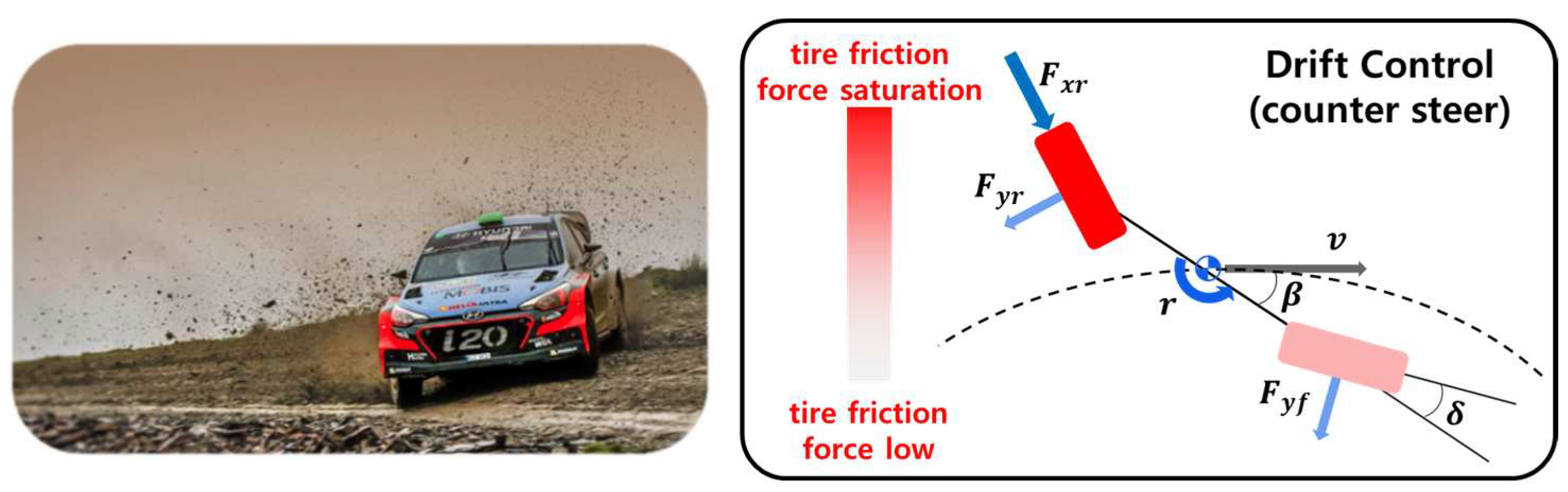
1. Introduction

To maximize passenger safety, future autonomous vehicles will be required to operate in various road environments and cope with various emergencies. A common emergency situation is high lateral slippage of the rear wheels on a sharply curved path or an ice-covered road, which leads to oversteering (see Figure 1). In such a situation, an autonomous vehicle should be capable of guaranteeing safety.

Drift technology (Figure 2) is a vehicle control strategy developed for use in motorsports. This technology enables professional racecar drivers to quickly generate high yaw rates that cannot be achieved with normal steering maneuvers. Such a driving technique requires expert driving skills to handle the vehicle’s behavior at its dynamic limit. Additionally, it is also used as a method for maintaining vehicle stability when an unintentional oversteering phenomenon occurs while driving.

Drift control methods for autonomous vehicles have been extensively studied. For example, the University of California, Berkeley [1] and Stanford University [2,3] have been developing drift control methods for several years. However, most existing control methods are based on the drift equilibrium state derived from vehicle dynamics. In particular, methods have been proposed to control a vehicle using a counter-steering maneuver that turns the steering wheel opposite to the turning direction [4,5]. Recent studies have introduced reinforcement learning techniques for developing drift control algorithms [6].

A drift control algorithm based on a nonlinear model predictive control (NMPC) method was also developed, which is a method using real-time numerical optimization to compute the control inputs minimizing the cost function [7,8].

In general, NMPC is based on real-time optimization techniques over a finite future horizon. The NMPC approach has many advantages; for instance, it considers the input and state constraints along with the dynamics during numerical optimization. However, the unpredictable computational time of most numerical optimization algorithms has limited the performance of NMPC in real-time control applications. To overcome this limitation, this study proposes a drift controller based on a deep neural network (DNN) algorithm. The proposed controller learns from data generated using the model predictive control (MPC) technique and demonstrates similar control performance as NMPC while delivering better real-time performance.

With the continued development of algorithms and computing devices, artificial intelligence (AI) is now being applied to various industrial applications. In automated vehicle research, AI advances enhance the integrity and safety of automated vehicle software. AI is also expected to serve as a solution for critical safety scenarios that are difficult to manage with conventional approaches [9,10].

The development of AI techniques that could improve the existing control systems has been addressed in several studies in various contexts. In particular, the performance of existing control systems has been improved by learning the driving from the data, enabling shared control between a driver and an autonomous driving system [11].

Other studies have attempted to increase the online performance of proportional integral derivative controllers by learning through an artificial neural network (ANN) [12,13,14]. Recently, primal-dual NNs have improved the real-time performance and stability of MPC [15].

Several studies have been conducted to improve the performance of the controller by reducing the uncertainty of the model using an ANN. In particular, the performance of MPC can be significantly improved by learning from real-time data, which provide knowledge of the target model [16,17,18,19,20,21,22,23,24,25,26,27].

The present study develops an NMPC-based drift control method that accurately tracks the predefined trajectories of an automated vehicle by using an established vehicle model. The developed NMPC-based drift controller is then replaced by a DNN-based controller pretrained on the data generated from the previously designed closed-loop trajectories of the NMPC method.

By replacing the previously designed NMPC method with the proposed DNN-based controller, we avoid the need for complex numerical optimization of the vehicle control, thereby reducing the computational load. The computational time of the DNN-based controller is very small and predictable in general, once the training process is complete. However, the computational cost of the NMPC method is often high and very unpredictable because its optimization problem includes many free variables that must be explored under many constraints. By switching the iterative numerical optimization process with a fixed number of NN computational processes, real-time implementation of the final control algorithm on a cheaper controller platform can be achieved and the real-time performance of the control method can be guaranteed. The new technique is especially advantageous in safety-critical applications such as automated vehicle control [28,29,30,31].

The following sections describe the development process. Section 2 analyzes the vehicle dynamics that were used for the NMPC’s design, and the simulation is introduced. The vehicle model is based on a 1:10-scaled vehicle (the test platform for future research). Section 3 presents the NMPC design process under which the automated vehicle performs the drift maneuver while following the desired curved trajectories. Section 4 illustrates the closed-loop simulation results of the designed NMPC, and Section 5 presents the design of the DNN-based controller. The research conclusions are presented in Section 6.

2. Vehicle Dynamics Analysis

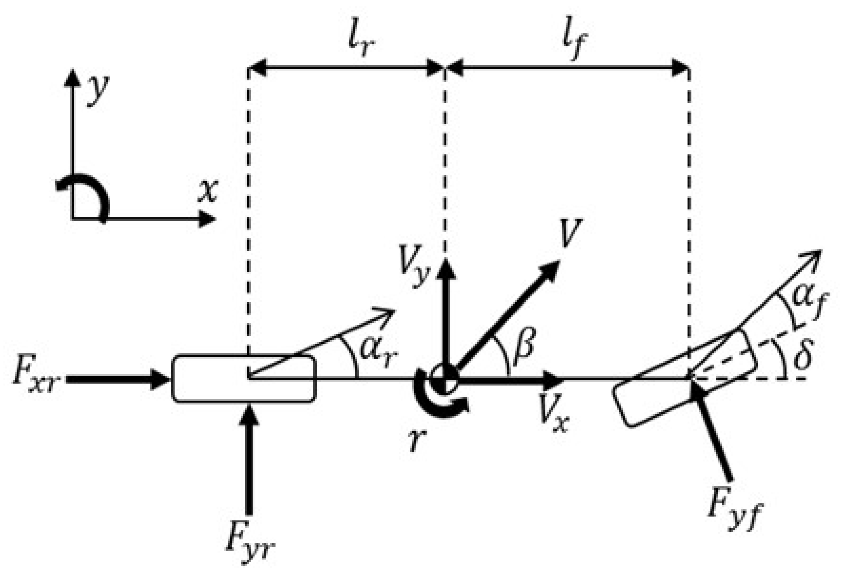
2.1. Three-Degrees-of-Freedom Bicycle Model

The horizontal motion of the vehicle was computed using the bicycle model shown in Figure 3. Neglecting aerodynamic drag forces, the bicycle model is defined as follows:

$$\begin{gathered} \dot{\beta }=\frac{F_{yf}\cos \left(\delta \right)+F_{yr}}{m}-r, \\ \dot{r}=\frac{F_{yf}\cos \left(\delta \right)-l_r{F}_{yr}}{I_{zz}}, \\ \dot{v_x}=\frac{F_{xr}-F_{yf}\sin \left(\delta \right)}{m}+r{v}_x\beta . \end{gathered}$$

(1)

Table 1. Nomenclature of the present study.

Symbol	Meaning	Unit
$F_{yf}$	Front tire lateral force	N
$F_{yr}$	Rear tire lateral force	N
$v$	Vehicle velocity	m/s
$v_w$	Rear-wheel velocity	m/s
$v_x$	Longitudinal velocity	m/s
$\mathsf{\alpha }$	Tire slip angle	rad
${\alpha }_f$	Front tire slip angle	rad
${\alpha }_r$	Rear tire slip angle	rad
$\mu$	Friction coefficient	-
${\mu }_s$	Friction coefficient of tire skids	-
$r$	Yaw rate	rad/s
$\delta$	Steering angle	rad
$\beta$	Sideslip angle	rad
$m$	Vehicle mass	kg
$l_f$	Distance from the center of gravity (CG) to the front axle	M
$l_r$	Distance from CG to the rear axle	M
$I_{zz}$	Yaw moment of inertia	N·m/rad2
$C_{xr}$	Rear tire longitudinal slip angle	-
$\kappa$	Tire slip ratio	-

defines the notations used in this study. The state variables of the vehicle model in Equation (1) are the sideslip angle ($\beta$), yaw rate ($r$), and forward velocity ($v_x$). The control inputs are the rear tire force ($F_{xr}$) and the steering angle ($\delta$).

2.2. Brush Tire Model

The longitudinal and lateral tire forces in the bicycle model are computed using a brush tire model, which constrains the maximum amount of tire force (the combined longitudinal and lateral forces) within the elliptical circle in Figure 4. A tire force curve versus the tire slip angle is illustrated in Figure 4, where the red area indicates the saturated area and the blue area denotes the unsaturated area. The brush tire model was employed using Equation (2).

$$\begin{gathered} F=\left\{\begin{array}{cc}\gamma -\frac{1}{3\mu F_z}{\gamma }^2+\frac{1}{27{\mu }^2{F}_z^2}{\gamma }^3,& \gamma \le 3\mu F_z\\ {\mu }_s{F}_z,& \gamma >3\mu F_z\end{array}\right., \\ {F}_x=\frac{C_x}{\gamma }\left(\frac{\kappa }{1+\kappa }\right)F, \\ {F}_y=\frac{C_{\alpha }}{\gamma }\left(\frac{tan\alpha }{1+\kappa }\right)F, \\ \mathsf{\gamma }=\sqrt{C_x^2{\left(\frac{\kappa }{1+\kappa }\right)}^2-C_{\alpha }^2{\left(\frac{tan\alpha }{1+\kappa }\right)}^2}, \\ \mathsf{\alpha }=\left\{\begin{array}{c}{\alpha }_f=atan\left(\frac{v_y+l_f\ast r}{v_x}\right)-\delta \approx atan\left(\beta +\frac{l_f}{v_x}\ast r\right)-\delta \\ {\alpha }_r=atan\left(\frac{v_y-l_r\ast r}{v_x}\right)\approx \mathrm{atan}\left(\beta -\frac{l_r}{v_x}\ast r\right)\end{array}\right., \\ \kappa =\frac{v_w-v_y}{v_x}. \end{gathered}$$

(2)

Under normal driving conditions, the combined force acting on a tire remains within the elliptic region and the tire model remains in the unsaturated state. Conversely, when the magnitude of the combined force acting on the tire reaches the elliptic circle, the tire model moves to the saturated state and a large amount of slip occurs. This situation is dangerous because the vehicle can lock its wheels or skid, which increases the difficulty of controlling the vehicle.

2.3. Drift Equilibrium State Analysis

The vehicle’s trajectory was predicted using the bicycle model defined in Equation (1) with speed and steering angle as the control inputs. To analyze the motion and stability of the vehicle, the bicycle model was combined with the brush tire model under specific conditions (Equation (2)). When the tire slip angle remains within a specific range and the tire force is unsaturated, the vehicle’s motion will remain stable. However, when the tire slip angle increases and the resulting tire force becomes saturated, the vehicle’s motion will destabilize and even a slight disturbance will divert its states from equilibrium.

To maintain the drift maneuver, the vehicle must be controlled in an unstable equilibrium state. Especially on a slippery road, maintaining a drift maneuver requires a precise and agile controller.

In this study, the equilibrium states were established using Equations (1) and (2) when the time derivatives of the vehicle’s states were all zero.

Figure 5 plots the $\beta$, $r$, and $v_x$ equilibrium points according to the steering angle at a longitudinal speed of 1.7 m/s. Plotted are the equilibrium states during a normal driving maneuver (*) and during a drift maneuver (o, Δ) in the clockwise and counterclockwise directions.

3. Design of the Nonlinear Model Predictive Controller

3.1. Vehicle State Prediction Model

Based on the dynamics of the controlled system, the NMPC method predicts the future motions of a vehicle over a fixed time horizon. In this study, the future trajectory was predicted by discretizing the model of the vehicle’s dynamics (Equation (1) in Section 2). The vehicle states ($X$) comprise the sideslip angle ($\beta$), yaw rate ($r$), and speed ($v_x$) of the vehicle as follows:

$$X=\left[\beta ,r,v_x\right].$$

(3)

The control input vector ($u$) comprises the rear-wheel speed ($v_w$) and the steering angle ($\delta$) of the vehicle.

$$u=\left[v_w,\delta \right].$$

(4)

In terms of the rear-wheel speed $(v_w)$, the rear-wheel tire force in Equation (1) is given by the following simplified tire force relation:

$$F_{xr}=\frac{C_{xr}\left(v_w-v_x\right)}{v_x}.$$

(5)

3.2. Nonlinear Model Predictive Controller Cost Function

The cost function for the optimization process of the NMPC method is the error vector ($X_k^e$) between the current vehicle state vector ($X_k$) and the target state vector ($X_k^{ref}$).

$$\begin{gathered} X_k^e=X_k^{ref}-X_k \\ =\left[{\beta }_k^{ref}-{\beta }_k, r_k^{ref}-r_k, v_{x_k}^{ref}-v_{x_k}\right]. \end{gathered}$$

(6)

The cost function (J) is defined in terms of the state error vectors and the control inputs.

$$J=\frac{1}{2}{\left(X_{k+N}^e\right)}^{\mathrm{T}}\ast P\ast X_{k+N}^e+\frac{1}{2}{\displaystyle \sum }_{j=k}^{k+N-1}{\left(X_j^e\right)}^{\mathrm{T}}\ast Q\ast X_j^e+u_j^{\mathrm{T}}R{u}_j.$$

(7)

Note that the cost function comprises a quadratic term of the final Nth step error ($X_N^e$), the sum of the quadratic terms of errors ($X_k^e$), and the quadratic terms of the control input ($u_k$) in future steps from k to k + N – 1, with weight matrices of P, Q, and R, respectively. The inputs that minimize the cost function given by Equation (7) are determined by numerical optimization based on a conjugate gradient method.

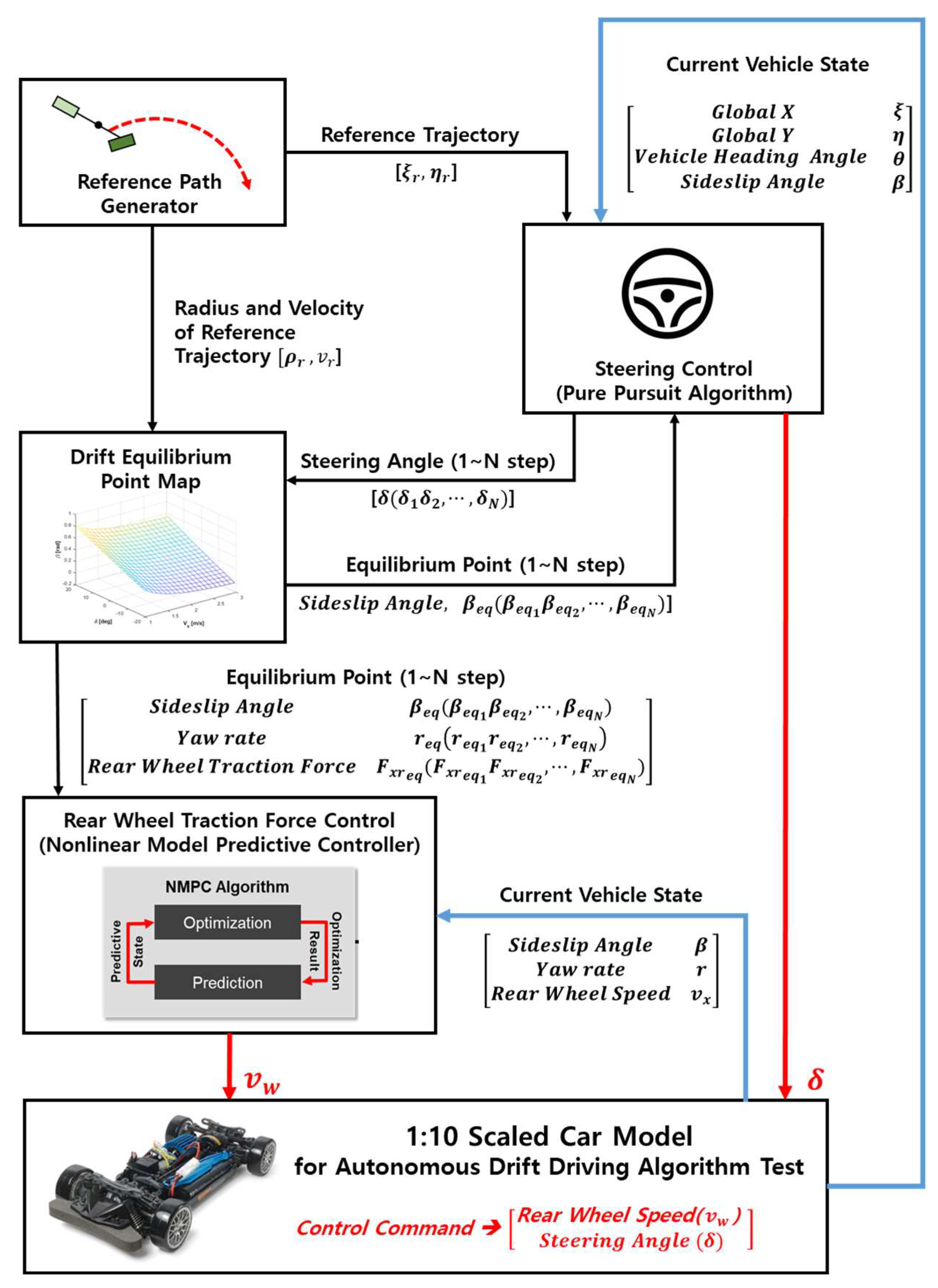
3.3. Nonlinear Model Predictive Controller System for Drift Driving

Figure 6 shows the control system of the developed NMPC-based drift control method. First, the curvature (${\rho }_r$) and reference speed ($v_r$) of the driving trajectory are provided by a path-generation algorithm. The drift equilibrium state is then obtained from the three-dimensional (3D) maps shown in Figure 7. Given the vehicle speed and steering angle at each time step, the 3D maps are configured to output the equilibrium states, i.e., ${\beta }_{eq},r_{eq}$, and $F_{x{r}_{eq}}$, based on the equilibrium analysis presented in Section 2.

The drift equilibrium points obtained from the 3D maps were assembled into the target state vector of the NMPC. The rear-wheel speed, $v_w$, that allows the vehicle to maintain the drift maneuver was calculated with the developed NMPC algorithm.

While maintaining the drift condition through rear-wheel control using the NMPC, an additional pure pursuit algorithm was used as the steering-angle controller to follow the desired trajectory. Similar to the NMPC, the pure pursuit algorithm inputs the current vehicle position and the target trajectory and computes the steering angle ($\delta$) from future time steps k to k + N. Figure 8 illustrates the path-following implementation of the pure pursuit control algorithm.

In the pure pursuit control algorithm, the waypoints are determined from the center point of the rear-wheel axis, which is switched to the center point of the vehicle to simplify the control law. Each waypoint is located at distance $l_d^{\prime }$ along the straight line in the direction of the target body’s sideslip angle. The vehicle’s trajectory over N future steps was computed using Equation (1), and the front-wheel steering angles up to N future steps were calculated as

$$\begin{gathered} {\delta }_k=\mathrm{atan}\frac{2Lsin{\beta }_k^{eq}}{l_d^{\prime }}+k_{\beta }{e}_{{\beta }_k} \\ =\mathrm{atan}\left(\frac{2Lsin{\theta }_k}{l_d^{\prime }}\right)+k_{\beta }\left({\beta }_k^{eq}-{\beta }_k\right). \end{gathered}$$

(8)

The first term in Equation (8) represents the control input that allows the vehicle to head toward the waypoints, and the second term represents the control input for creating the vehicle’s track, i.e., ${\beta }_{eq}$. To obtain the future equilibrium states followed by the NMPC, the steering-angle inputs from the pure pursuit control algorithm are applied to the 3D drift equilibrium maps.

4. Drift-Driving Test of the Nonlinear Model Predictive Controller

4.1. Test Scenario

The performance of the NMPC-based drift control method was evaluated through numerical simulations. The controller was required to follow 8-shaped trajectories with diameters of 2 m (① and ②) and 2.5 m (③ and ④), as shown in Figure 9.

The control period and NMPC prediction period were set to 50 Hz (0.02 s) and 20 steps, respectively. Under these settings, the NMPC system can predict the maneuver for 0.4 s.

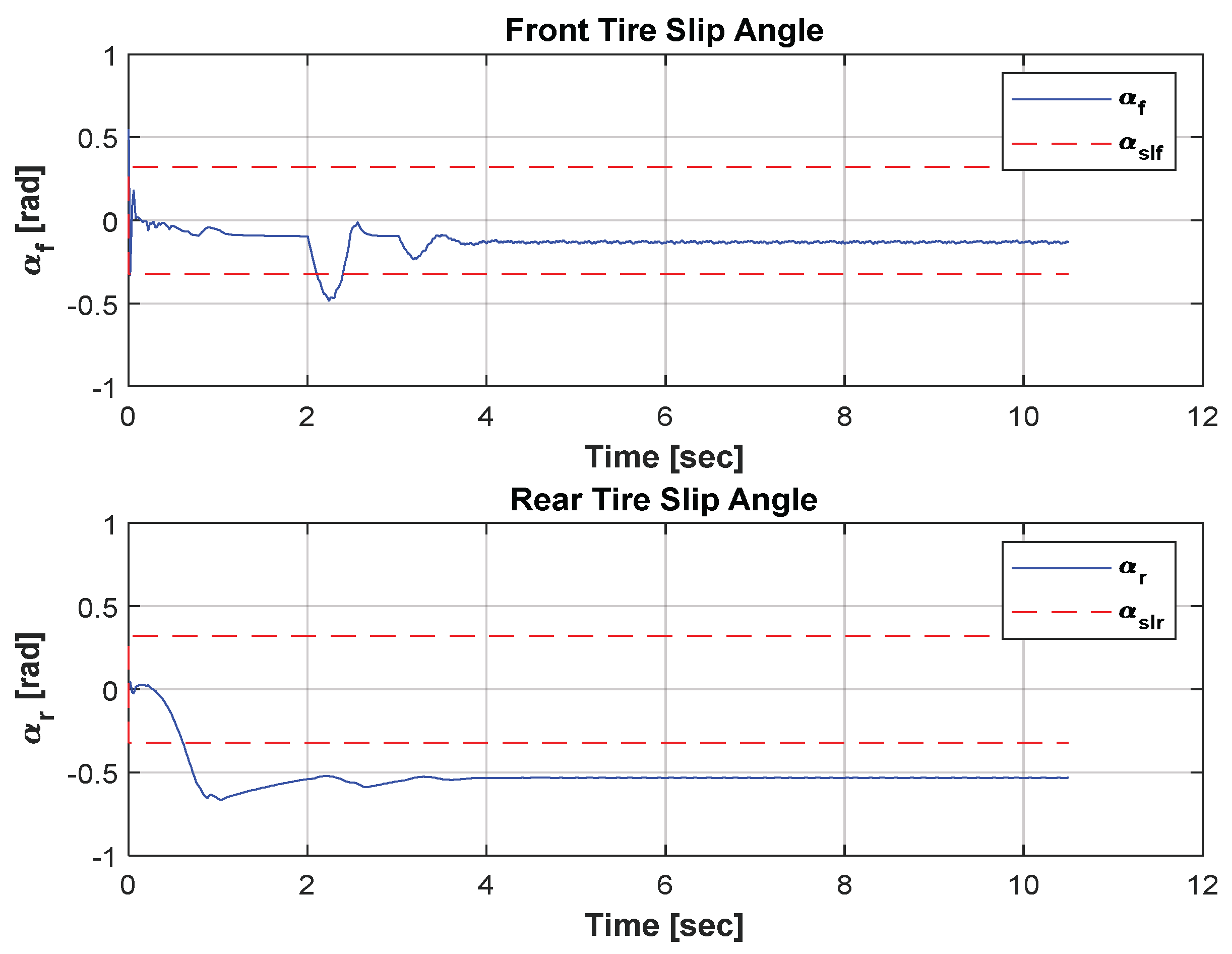
4.2. Drift Test Results

In the test scenario, the test vehicle was controlled to drive on routes ①–④ repeatedly using the drift maneuver. Figure 10 shows the sideslip angle and yaw rate ($\beta$ and $r$, respectively) of the vehicle during the simulation. In scenarios ① and ③, the vehicle drove in the counterclockwise direction; hence, its body sideslip angle was negative and its yaw rate was positive. Conversely, in scenarios ② and ④, the vehicle drove in the clockwise direction with a positive body sideslip angle and a negative yaw rate. The designed NMPC method accurately followed the desired sideslip angle and yaw rate provided by the 3D map.

As shown in Figure 11, the front tire slip never exceeded the limit but the rear tire slip did. Therefore, the front-wheel steering controller required a control-force margin to maintain the desired trajectory, whereas the rear-wheel controller successfully maintained the drift condition by following the desired angle and yaw rate.

Figure 12 shows the driving trajectory of the NMPC-based drift-driving control method. The vehicle precisely followed the figure-eight-shaped target trajectory.

5. Design of the Neural Network Drift Controller

The NMPC method predicts a vehicle’s behavior up to a predetermined future time and derives the optimal control inputs through numerical optimization with a predesigned cost function. A notable advantage of this method is consideration of the characteristics (dynamics and constraints) during the system optimization. On the downside, accounting for these constraints significantly increases the computational time of the optimization, which is undesirable in fast real-time control applications.

To overcome these limitations while exploiting the advantages of the developed NMPC method, this study employed a DNN-based control method that uses the driving data generated by the NMPC method during drift behavior.

5.1. Training Data Preprocess

The DNN was trained on approximately 50,000 sets of simulated trajectory-driving data, collected along the 2-m-diameter path in Figure 10 (counterclockwise driving along Path ①).

Because the vehicle states, such as vehicle velocity and sideslip angle, have different units and magnitudes, the data were preprocessed by normalizing as follows:

$$x_{norm}=\frac{x-x_{min}}{x_{max}-x_{min}},$$

(9)

where $x$ represents the variable to be normalized and $x_{min}$ $\mathrm{and} x_{max}$ represent the minimum and maximum values, respectively, among the sets of variables x. To increase the efficiency of the learning process, only data within the normal range were selected. The standard score $z$ was thus defined as follows:

$$z=\frac{x-\mu }{\sigma },$$

(10)

where $\mu$ and $\sigma$ signify the mean and standard deviation of the data, respectively.

If the absolute value of the Z score exceeded 2, the datum was excluded from the training data because it was outside the normal range of 95% probability. In this process, the data were assumed to follow a Gaussian distribution. The data normalization results are shown in

Table 2. Training data for steering (lateral) control.

		Mean and Standard Deviation		Normalization Variables
		$\mathit{\mu }$	$\mathit{\sigma }$	Min	Max
Input Data	$x_e$*	−0.0307	0.1819	−0.2697	0.2674
	$y$†	0.0080	0.2070	−0.2688	0.2695
	$\beta$	−0.4278	0.1314	−0.5625	−0.3534
	${\beta }_{eq}$o	−0.4969	0.1213	−0.6379	−0.2630
Output Data	$\delta$	−0.1742	0.1216	−0.3876	0.0651

* Longitudinal position error with respect to the reference point; ^† Lateral position error with respect to the reference point; ^o Sideslip angle equilibrium point.

and

Table 3. Training data for steering (longitudinal) control.

		Mean and Standard Deviation		Normalization Variables
		$\mathit{\mu }$	$\mathit{\sigma }$	Min	Max
Input Data	$v_x$	−0.0307	0.1819	−0.2697	0.2674
	$v_y$	0.0080	0.2070	−0.2688	0.2695
	$\beta$	−0.4278	0.1314	−0.5625	−0.3534
	$r$	−0.4969	0.1213	0.6379	0.2630
Output Data	$v_w$ *	−0.1742	0.1216	−0.3876	0.0651

* Vehicle’s rear-wheel speed.

.

As an example, Figure 13 presents the data before and after normalizing the sideslip angle. The data were distributed in the range of −0.48–0.43 before normalization (left panel) and the range 0 to 1 after normalization (right panel).

5.2. Neural-Network-Based Controller Architecture

The control system architecture includes two NN controllers (Figure 14). The first NN controller, based on a DNN, controls the steering wheel to drive the vehicle along the desired trajectory during a drift maneuver. The second NN controller, based on a time delay NN (TDNN), maintains the drift state of the vehicle.

5.2.1. Deep Neural-Network-Based Controller for Steering Control

A typical NN comprises an input layer, one or more hidden layers, and an output layer. To include the characteristics of the system and prevent unstable behavior due to external disturbances [26,27], the present study employed a DNN with six hidden layers. Each of the six hidden layers was configured with 20 artificial neural nodes as shown in Figure 15. The input data of the network (Table 2) include the position error ($x_e,y_e$) between the path point and the vehicle, the body slip angle ($\beta$), and the body slip-angle equilibrium point (${\beta }_{eq}$) generated from the 3D map. The network outputs the vehicle steering angle ($\mathsf{\delta }$) for lateral position control.

5.2.2. Time Delay Neural-Network-Based Controller for Drift State Control

The designed NMPC method for maintaining the drift equilibrium states was replaced with a TDNN-based controller. To include the dynamic characteristics of the vehicle during the drift maneuver, the network structure must reflect the near-past vehicle states. The TDNN structure inputs the current data and the data of the past four steps (t, t−1, t−2, t−3, and t−4) as follows:

$$\begin{gathered} \mathrm{Current} \mathrm{States}: X^t=\left[v_x^t,v_y^t,{\beta }^t,r^t\right], \\ \mathrm{Previous} \mathrm{States}: X^{t-1}=\left[v_x^{t-1},v_y^{t-1},{\beta }^{t-1},r^{t-1}\right], \\ ⋮ \\ {X}^{t-4}=\left[v_x^{t-4},v_y^{t-4},{\beta }^{t-4},r^{t-4}\right], \end{gathered}$$

(11)

$$\mathrm{Input} \mathrm{Data}: \mathrm{I}=\left[X^t,X^{t-1},X^{t-2},X^{t-3},X^{t-4}\right],$$

(12)

where the number of time delay steps was set to 4. The TDNN-based drift controller (Figure 16) contains six hidden layers, each holding 20 artificial neural nodes.

The TDNN inputs were the longitudinal and lateral speeds ($v_x,v_y$), body slip angle ($\beta$), and rotation angular speed ($r$) in Table 3 and the output was the rear-wheel speed ($v_w$). The DNN was trained on ~50,000 sets of simulation data obtained from the trajectory-driving data (counterclockwise driving around the 2-m-diameter path; see ① in Figure 10).

6. Simulation Results of the Neural Network Drift Controller

The performance of the DNN-based drift control method was evaluated through numerical simulations of a 1:10-scale vehicle driving counterclockwise around a 1-m-radius circle. In this scenario, the vehicle speed was set to 1.7 m/s.

Figure 17 shows the sideslip angles of the front and rear wheels during the drift maneuver. The lateral slip of the front tire did not exceed the saturation limit, whereas the lateral slip of the rear tire exceeded the saturation limit while maintaining the drift condition, allowing the rapid increase of yaw rate that is necessary for following the 1-m-radius circular path. The same phenomenon was observed during the closed-loop simulation using NMPC.

Figure 18 plots the vehicle states during the drift maneuver. Although the TDNN-based rear-wheel controller did not explicitly use the 3D map information of the vehicle equilibrium states, the desired equilibrium points are also plotted as a reference.

The vehicle’s states accurately followed the desired equilibrium states of the body sideslip angle, yaw rate, and longitudinal velocity, even though the TDNN-based controller does not explicitly have information related to the 3D map. It was concluded that the closed-loop trajectory data generated by the NMPC implicitly included information on the drift equilibrium states, which was transferred to the TDNN-based controller during the learning process.

Figure 19 and Figure 20 display the closed-loop trajectory of the vehicle controlled by the TDNN and the tracking errors, respectively. The mean lateral position error remained at ~0.06 m during the drift maneuver. The designed DNN-based steering controller accurately followed the desired trajectory.

7. Conclusions

In this study, a drift control method for autonomous vehicles was developed as a strategy for managing a dangerous oversteer phenomenon that may occur during driving. First, a NMPC-based drift controller was designed by analyzing the tire model and vehicle dynamics during the drift maneuver. The closed-loop performance of the developed NMPC method was evaluated through numerical simulations of figure-eight-shaped vehicle trajectories with different radii.

Second, a data-driven NN-based control method was employed to overcome the limitations of the real-time performance of the existing NMPC-based drift controller. The DNN- and TDNN-based controllers incorporated the closed-loop performance of the previously designed NMPC method by learning the trajectories and input data obtained from the simulations. The performance of the developed data-driven controller was further verified through realistic numerical simulations, which confirmed the accurate tracking performance of the vehicle along a circular path.

Based on the study results, the proposed data-driven control method has the potential to be used as a controller for autonomous vehicles. The method retains the advantages of the sophisticated model-based NMPC approach for managing expert driving techniques such as drift. In addition, it can learn expert driving skills from a broad range of user data, potentially overcoming the limitations of the current rule-based autonomous driving system.

References

- Zhang, F.; Gonzales, J.; Li, S.E.; Borelli, F.; Li, K. Drift Control for Cornering Maneuver of Autonomous Vehicle. Mechatronics 2018, 54, 164–174. [Google Scholar] [CrossRef]
- Hindiyeh, R.Y. Dynamics and Control of Drifting in Automobiles. Ph.D. Thesis, Department of Mechanical Engineering, Stanford University, Stanford, CA, USA, 2013. [Google Scholar]
- Goh, J.Y.; Goel, T.; Gerdes, J.C. Towards Automated Vehicle Control Beyond the Stability Limits: Drifting Along a General Path. J. Dyn. Syst. Meas. Control 2020, 142, 02004. [Google Scholar] [CrossRef]
- Park, M.; Kang, Y. Experimental Verification of a Drift Controller for Autonomous Vehicle Tracking: A Circular Trajectory Using LQR Method. Int. J. Control Autom. Syst. 2021, 19, 404–416. [Google Scholar] [CrossRef]
- Kim, M.; Lee, T.; Kang, Y. Experimental Verification of the Power Slide Driving Technique for Control Strategy of Autonomous Race Cars. Int. J. Precis. Eng. Manuf. 2020, 21, 377–386. [Google Scholar] [CrossRef]
- Cai, P.; Mei, X.; Tai, L.; Sun, Y.; Liu, M. High-Speed Autonomous Drifting with Deep Reinforcement Learning. IEEE Robot. Autom. Lett. 2020, 5, 1247–1254. [Google Scholar] [CrossRef]
- Guo, H.; Tan, Z.; Liu, J.; Chen, H. MPC-based Steady-state Drift Control under Extreme Condition. In Proceedings of the 33rd Chinese Control and Decision Conference (CCDC), Kunming, China, 22–24 May 2021; pp. 4708–4721. [Google Scholar]
- Xu, D.; Han, Y.; Ge, C.; Qu, L.; Zhang, R.; Wang, G. A Model Predictive Control Method for Vehicle Drifting Motions with Measurable Errors. World Electr. Veh. J. 2022, 13, 54. [Google Scholar] [CrossRef]
- Hristozov, A. The Role of Artificial Intelligence in Autonomous Vehicles. Available online: https://www.embedded.com/the-role-of-artificial-intelligence-in-autonomous-vehicles/ (accessed on 15 July 2020).
- Hristozov, A. Artificial Intelligence Algorithms and Challenges for Autonomous Vehicles. Available online: https://www.embedded.com/artificial-intelligence-algorithms-and-challenges-for-autonomous-vehicles/ (accessed on 3 August 2020).
- Huang, M.; Gao, W.; Wang, Y.; Jiang, Z. Data-Driven Shared Steering Control of Semi-Autonomous Vehicles. IEEE Trans. Hum.-Mach. Syst. 2019, 49, 350–361. [Google Scholar] [CrossRef]
- Zribi, A.; Chtourou, M.; Djemel, M. A New PID Neural Network Controller Design for Nonlinear Processes. J. Circuits Syst. Comput. 2018, 27, 1850065. [Google Scholar] [CrossRef]
- Chertovskikh, P.; Seredkin, A.; Godyzov, O.; Styuf, A.; Pashkevich, M.; Tokarev, M. An Adaptive PID Controller with an Online Auto-tuning by a Pretrained Neural Network. J. Phys. Conf. Ser. 2019, 1359, 15–22. [Google Scholar] [CrossRef]
- Yaadav, A.; Gaur, P. AI-based Adaptive Control and Design of Autopilot System for Nonlinear UAV. Indian Acad. Sci. 2014, 39, 765–783. [Google Scholar] [CrossRef] [Green Version]
- Jhang, X.; Bujarbaruah, M.; Borrelli, F. Safe and Near-Optimal Policy Learning for Model Predictive Control Using Primal-Dual Neural Networks. In Proceedings of the IEEE American Control Conference (ACC), Philadelphia, PA, USA, 10–12 July 2019; pp. 354–359. [Google Scholar]
- Rankovic, V.; Radulovic, J.; Grufovic, N.; Divac, D. Neural Network Model Predictive Control of Nonlinear Systems Using Genetic Algorithms. Int. J. Comput. Commun. Control 2012, 7, 540–549. [Google Scholar] [CrossRef]
- Shi, T.; Wang, P.; Chan, C.; Zou, C. A Data Driven Method of Optimizing Feedforward Compensator for Autonomous Vehicle. IEEE Intell. Veh. Symp. 2019, 1901, 2012–2017. [Google Scholar]
- Vasikaninová, A.; Bakošová, M. Neural Network Predictive Control of a Chemical Reactor. Acta Chim. Slovaca 2009, 2, 21–36. [Google Scholar]
- Zhang, Z.; Wu, Z.; Rincon, D.; Christofides, P. Real-Time Optimization and Control of Nonlinear Processes Using Machine Learning. Mathematics 2019, 7, 890. [Google Scholar] [CrossRef]
- Wong, W.; Chee, E.; Li, J.; Wang, X. Recurrent Neural Network-Based Model Predictive Control for Continuous Pharmaceutical Manufacturing. Mathematics 2018, 6, 242. [Google Scholar] [CrossRef]
- Ramdane, H. Adaptive Neural Network Model Predictive Control. Int. J. Innov. Comput. Inf. Control 2013, 9, 1245–1257. [Google Scholar]
- Limon, D.; Calliess, J.; Maciejowski, J.M. Learning-based Nonlinear Model Predictive Control. IFAC-PapersOnLine 2017, 50, 7769–7776. [Google Scholar] [CrossRef]
- Afram, A.; Sharifi, F.J.; Fung, A.S.; Raahemifar, K. Artificial Neural Network (ANN) Based Model Predictive Control (MPC) and Optimization of HVAC systems: A state of the Art Review and Case Study of a Residential HVAC System. Energy Build. 2017, 141, 96–113. [Google Scholar] [CrossRef]
- Gonzalez, L.P.; Sanchez, S.S.; Guzuman, J.G.; Boada, M.J.L.; Boada, B.L. Simultaneous Estimation of Vehicle Roll and Sideslip Angles through a Deep Learning Approach. Sensors 2020, 20, 3679. [Google Scholar] [CrossRef]
- Mohamed, I.; Rovetta, S.; Do, T.; Dragicević, T.; Diab, A. A Neural Network Based Model Predictive Control of Three-Phase Inverter with an Output LC Filter. IEEE Access 2019, 7, 124737–124749. [Google Scholar] [CrossRef]
- Peng, H.; Song, N.; Li, F.; Tang, S. A Mechanistic-Based Data-Driven Approach for General Friction Modeling in Complex Mechanical System. ASME J. Appl. Mech. 2022, 89, 071005. [Google Scholar] [CrossRef]
- Peng, H.; Song, N.; Kan, Z. Data-Driven Model Order Reduction with Proper Symplectic Decomposition for Flexible Multibody System. Nonlinear Dyn. 2022, 107, 173–203. [Google Scholar] [CrossRef]
- Kang, B.; Lucia, S. Learning-based Approximation of Robust Nonlinear Predictive Control with State Estimation Applied to a Towing Kite. In Proceedings of the 18th European Control Conference (ECC), Naples, Italy, 25–28 June 2019; pp. 16–22. [Google Scholar]
- Lee, T.; Kang, Y. Performance Analysis of Deep Neural Network Controller for Autonomous Driving Learning from a Nonlinear Model Predictive Control Method. Electronics 2021, 10, 767. [Google Scholar] [CrossRef]
- Winkler, D.A.; Le, T.C. Performance of Deep and Shallow Neural Networks, the Universal Approximation Theorem, Activity Cliffs, and QSAR. Mol. Inform. 2017, 36, 1–2. [Google Scholar]
- Lucia, S.; Karg, B. A Deep Learning-based Approach to Robust Nonlinear Model Predictive Control. IFAC-PapersOnLine 2018, 51, 511–516. [Google Scholar] [CrossRef]