Abstract
Since its 3.3 release, Modelica offers the possibility to specify models of dynamical systems with multiple modes having different DAE-based dynamics. However, the handling of such models by the current Modelica tools is not satisfactory, with mathematically sound models yielding exceptions at runtime. In this article, we propose several contributions to this multifaceted issue, namely: an efficient and scalable multimode extension of the structural analysis of Modelica models; a systematic way of rewriting a multimode Modelica model, based on this analysis, so that the rewritten model is guaranteed to be correctly compiled by state-of-the-art Modelica tools; a proposal for the handling of the consistent initialization of multimode models; multimode structural analysis algorithms that handle both multiple modes and mode change events in a unified framework, coupled with a compile-time algorithm for identifying and quantifying impulsive behaviors at mode changes. Our approach is illustrated on relevant example models, and the performance of our implementations is assessed on a variable dimension large-scale model.
1. Introduction
Modelica and other languages supporting object-oriented modeling of physical systems rely on the formalism of Differential Algebraic Equations, or DAEs. Compilers of such languages perform sophisticated preprocessing prior to generating simulation code [1]. Index analysis and reduction [2] is one such important processing, where selected equations are differentiated one or more times so that the Jacobian matrix with respect to the leading variables (i.e., the variables of maximal differentiation degree in the system) becomes regular. This is typically performed by using so-called structural analysis methods, such as the Pantelides algorithm [3] and Pryce’s -method [4].
Since its 3.3 release, the Modelica language offers the possibility of specifying multimode dynamics, by describing state machines with different DAE dynamics in each different state [5]. Multimode DAEs, or mDAEs, can thus be written in the Modelica language. This valuable feature enables describing large and complex cyberphysical systems with different behaviors in different modes. Unfortunately, multimode modeling has been the source of serious difficulties for non-expert users of the current generation of Modelica tools. Indeed, while many large-scale Modelica models are properly handled, some physically meaningful models do not result in correct simulations with most tools. As such problematic models are actually easy to construct, the likelihood of such bad cases occurring in large models is significant.
It is unfortunately unclear which multimode Modelica models will be properly handled, and which ones will fail. As a consequence, quite often, end users have to ask Modelica experts, or even tool developers themselves, to tweak their models in order to make them work as expected. While it is accepted that physical modeling itself requires expertise, requiring expertise in how to get around tool idiosyncrasies is not desirable. This situation hinders a wider spreading of Modelica tools among a larger class of users, such as Simulink-trained engineers.
More than 10 years ago, we initiated a project addressing the handling of multimode models by Modelica tools. We showed how the issues discussed above mainly boil down to inadequate structural analysis of multimode models: as far as we know, no industrial-strength Modelica tool implements a mode-dependent structural analysis; worse, it is not even understood what kind of structural analysis should be associated with mode change events.
We already proposed several contributions to the structural analysis of multimode models. In [6], we introduced efficient algorithms for the structural analysis of multimode models in an “all-modes-at-once” fashion and presented promising experimental results for a prototype implementation named IsamDAE. In [7], we proposed a structural analysis that is valid for multimode DAE models, both within each mode and at mode changes, with an additional focus on possible impulsive behaviors that appear at mode changes in many physical models. These works were explained, with a more practical standpoint, in the three papers [8,9,10]. In addition to casting the above contributions into a coherent perspective, this article brings new structural analysis algorithms, thus proposing a comprehensive range of tools for the correct compilation of multimode Modelica models.
One can distinguish between four phases (Our approach supports multimode Modelica models exhibiting only these four phases. In particular, we do not support models exhibiting so-called “sliding modes” [11], in which the system bounces back and forth between two or several DAE dynamics in zero time, for some positive duration) in the simulation of a multimode Modelica model:
- Initialization, in which initial conditions consistent with the multimode DAE system must be specified;
- Long modes, which are modes lasting for some positive duration, each one being governed by a specific DAE dynamics;
- Mode changes, which are events separating two successive long modes and possibly requiring a specific reset of the state of the system;
- Transient modes, which are modes with zero duration in which a specific dynamics is in force; such modes can occur in finite sequences called cascades. Transient modes occur, for example, with elastic impacts in contact mechanics: this is illustrated below by the Cup-and-Ball game example, a multimode variation of the celebrated pendulum in Cartesian coordinates.
It turns out that these four different phases of the multimode dynamics require different structural analyses.
For long modes, classical structural analysis methods for DAEs apply; the same holds for consistent initialization, which actually was the core motivation for the seminal work of Pantelides [3]. However, in both cases, one problem has to be solved for each long mode and each possible initial mode of the system, which cannot be performed by enumeration. Part of the works presented in this paper addresses efficient methods for the mode-dependent structural analysis of both the long modes and initial modes.
As for mode changes and transient modes, they require novel structural analyses that were not considered before in a multi-physics or physics-agnostic context. For mode changes, the core issue is the conflict that can occur between the DAE dynamics before and after the mode change; this possible conflict is due to the fact that the restart conditions in the new mode are influenced by both dynamics. The structural analysis of finite cascades of transient modes even requires further care, as we shall see.
All these structural analyses are meant to work together, as components of a compile-time structural analysis chain for mDAE models. Their results are complementary, in that they provide the information needed for generating correct and efficient code for all four phases of the simulation. To our knowledge, no such works exist in the DAE literature.
It still has to be noted, however, that the methods presented in this article do not guarantee, in all generality, the numerical nonsingularity of the model. In other words, they share the limitations inherent in any structural analysis method, such as the Pantelides method [3], Pryce’s -method [4], and the dummy derivatives method [2]. Numerical methods for mDAEs is a highly relevant research topic, that falls outside of the scope of the works presented here. So-called symbolic-numeric methods [12,13,14] would be an interesting midway solution, although they are still unable to guarantee numerical nonsingularity.
The paper is organized as follows.
We first exhibit, in Section 2, three simple small-sized Modelica models that are not correctly handled by state-of-the-art Modelica tools, and we explain the reasons behind these failures. In Section 3, we go further by writing down a sensible physical model that would require extending the Modelica language. All four models are used throughout the article for either illustrating algorithms or assessing the performances of our implementation.
Section 4 introduces the symbolic representations we are using to alleviate the need for mode enumeration during the handling of multimode models. We also present two algorithmic building blocks, built on top of these representations, that constitute the basis for all of our contributions; namely, a multimode extension of the classical Dulmage–Mendelsohn decomposition of a system of algebraic equations [15], and a multimode extension of Pryce’s -method for the structural analysis of DAE systems [4]. The design of these algorithms is fit for handling variable dimension models such as the one introduced in Section 3 so that they could be used for designing compilers for useful extensions of the Modelica language.
Although these building blocks provide the bases for an efficient structural analysis of multimode systems, they are not quite sufficient for addressing the daunting challenge of scalability. Section 5 is dedicated to the CoSTreD (Constraint System Tree Decomposition) method, a novel generic approach for solving multimode constraint systems, that we apply to the building blocks introduced above. This method exploits model sparsity, a feature exhibited by most large-sized practical industrial models.
We explain in Section 6 how all these pieces are put together in the IsamDAE tool for the structural analysis of long modes of multimode DAE models, and we assess its correctness and scalability. We complement these results with the introduction, in Section 7, of the latest feature of IsamDAE, that is, an efficient multimode extension of the consistent initialization of DAE models.
Section 8 focuses on the structural analysis of mode changes and finite cascades of transient modes. This approach is based on nonstandard analysis [16,17], which allows for a grounded use of infinities and infinitesimals in mathematical analysis. Section 9 addresses the related issue of impulsive behaviors that may occur at mode changes. After the introduction of a simple illustrative example, we propose a general compile-time analysis for impulsive behaviors, designed to act as an additional step in the structural analysis of mode changes. This analysis can be used, in particular, to renormalize impulsive variables when implementing a numerical scheme that approximates the restart values for each state variable of the system, thus improving conditioning. The efficient implementation of these contributions in the IsamDAE tool is currently in progress.
Finally, Section 10 demonstrates how the results of the multimode structural analysis performed by the IsamDAE tool can be used for transforming a multimode Modelica model into its RIMIS (Reduced Index Mode-Independent Structure) form, which is guaranteed to yield correct execution in state-of-the-art Modelica tools. This approach is assessed on one of the examples introduced before, then formalized for its broad application to multimode models.
2. Multimode Modelica Models
Several constructs of the Modelica language enable the definition of switched or hybrid dynamical systems, often called multimode systems in the Modelica community. For instance, it is possible to use if-then-else conditional statements in equations, or equations can be themselves placed in such conditional statements. Hierarchical state machines [5] are also part of the Modelica language [18], enabling a higher-level, clearer modeling style for multimode systems.
However, with all these constructs come several difficult issues. From a mathematical perspective, it turns out that the existence and uniqueness of solutions of a multimode DAE system is a much more difficult question than for pure (or single-mode) DAEs, as detailed in [7]. As for the compilation of multimode Modelica models for the generation of simulation code, it is complicated by the fact that the structure of a multimode DAE system may depend on the mode, and may change at runtime whenever the system switches from one mode to another; as a result, convenient assumptions made by state-of-the-art Modelica tools for simplifying the compilation of such models can result in incorrect runtime behavior for many meaningful examples, as we shall see.
In this section, we review several models, from the simplest (with only two equations) in Section 2.1, to the physically relevant Water Tank example of Section 2.2 and the idealized, but not less relevant, clutch model of Section 2.3. For each of these models, we carry out an in-depth analysis of the difficulties encountered with Modelica tools such as OpenModelica [19] and Dymola [20]. This sheds light on the root causes of the limitations of these tools, and shows how a genuine multimode structural analysis could resolve these issues.
2.1. A Simple Two-Equation Model
A root cause of simulation failures with existing Modelica tools is highlighted by the model shown in Figure 1.
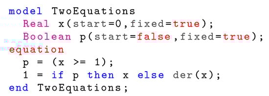
Figure 1.
Modelica model of a simple two-equation system.
This model only has one real equation and one Boolean equation, and it has no particular physical meaning. However, it captures, in a nutshell, the difficulty raised by numerous multimode models, including the Water Tank model introduced in Section 2.2 below. As a matter of fact, it’s numerical solving should proceed in different ways depending on the value of the Boolean variable p:
- When p is true, x is a leading variable, meaning that it is the unknown that needs to be solved;
- When p is false, the leading variable is x′, the first-order time derivative of x, while x itself is a state variable.
This information can be summarized in the form of a Conditional Dependency Graph (CDG), showing what blocks of equations have to be solved in which sets of modes. This graph can be obtained as the result of the multimode structural analysis performed by the IsamDAE tool, introduced in Section 6. The CDG resulting from the structural analysis of the two-equation model is shown in Figure 2a; in this figure, e denotes the real equation of the model. In general, the CDG also provides information about causal dependencies between blocks, but for this simple example, only one block has to be solved in each mode.

Figure 2.
CDG and DG of the two-equation model from Figure 1. Vertices are conditional equation blocks of the form p: , where: E is the block of equations; p is a Boolean condition, defining the set of modes in which the block has to be solved; R is a set of variables to read, or free variables, i.e., parameters of the block of equations; W is a set of variables to write, meaning that they are the unknowns of the block of equations. When R is empty, the shorthand notation is . When p is the constant , prefix “p:” is omitted. (a) CDG of the two-equation model, resulting from the multimode structural analysis; (b) DG of the two-equation model, resulting from the approximate structural analysis.
This mode-dependent structural analysis is not performed by Modelica tools such as OpenModelica 1.17.0 [19] and Dymola 2021 [20]. Instead, these tools rely on an approximate structural analysis, that omits mode dependencies in order to apply standard single-mode methods such as the Pantelides method [3] or Pryce’s -method [4]. More precisely, this approximate structural analysis is performed by abstracting away all mode dependencies inside the equations; for instance, an equation x = if cond then y else z will be regarded as an equation involving variables x, y and z. On the two-equation model, this results in the Dependency Graph (DG) given in Figure 2b.
The approximate structural analysis determines that the leading variable is x′ in all modes; however, the actual equation is singular in x′ when p is true. As a result, an exception is raised during simulation, as shown in Figure 3.
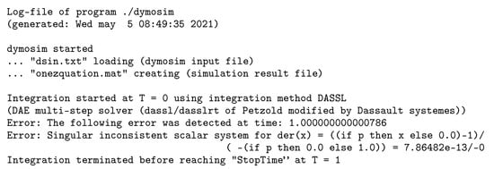
Figure 3.
Failed simulation of the two-equation model with Dymola 2021.
As such, this simple example shows how models in which the leading variables depend on the mode can be troublesome for Modelica tools. A genuine multimode Modelica compiler must be able to handle models for which the set of leading variables is mode-dependent.
2.2. A Simplified Water Tank Model
The Water Tank system is a simple model of a closed tank with a variable water inflow z and a default outflow y0, where water is considered incompressible. When the tank is full, a positive flow correction yh is added to the outflow, as the tank cannot store more water; conversely, when the tank is empty, a negative flow correction yl is added to the outflow.
The corresponding Modelica model, given in Figure 4, uses two complementarity conditions [21] for the flow corrections. The first one, encoded by the multimode equations eh1 and eh2, depends on the Boolean variable bh, which is true if and only if variable sh is nonnegative. The combined effect of these two equations is that xmax − x and yh are always nonnegative, and that at least one of those is equal to 0 at any time. Equations el1 and el2 encode the second complementarity condition (between x − xmin and yl) in a similar way.
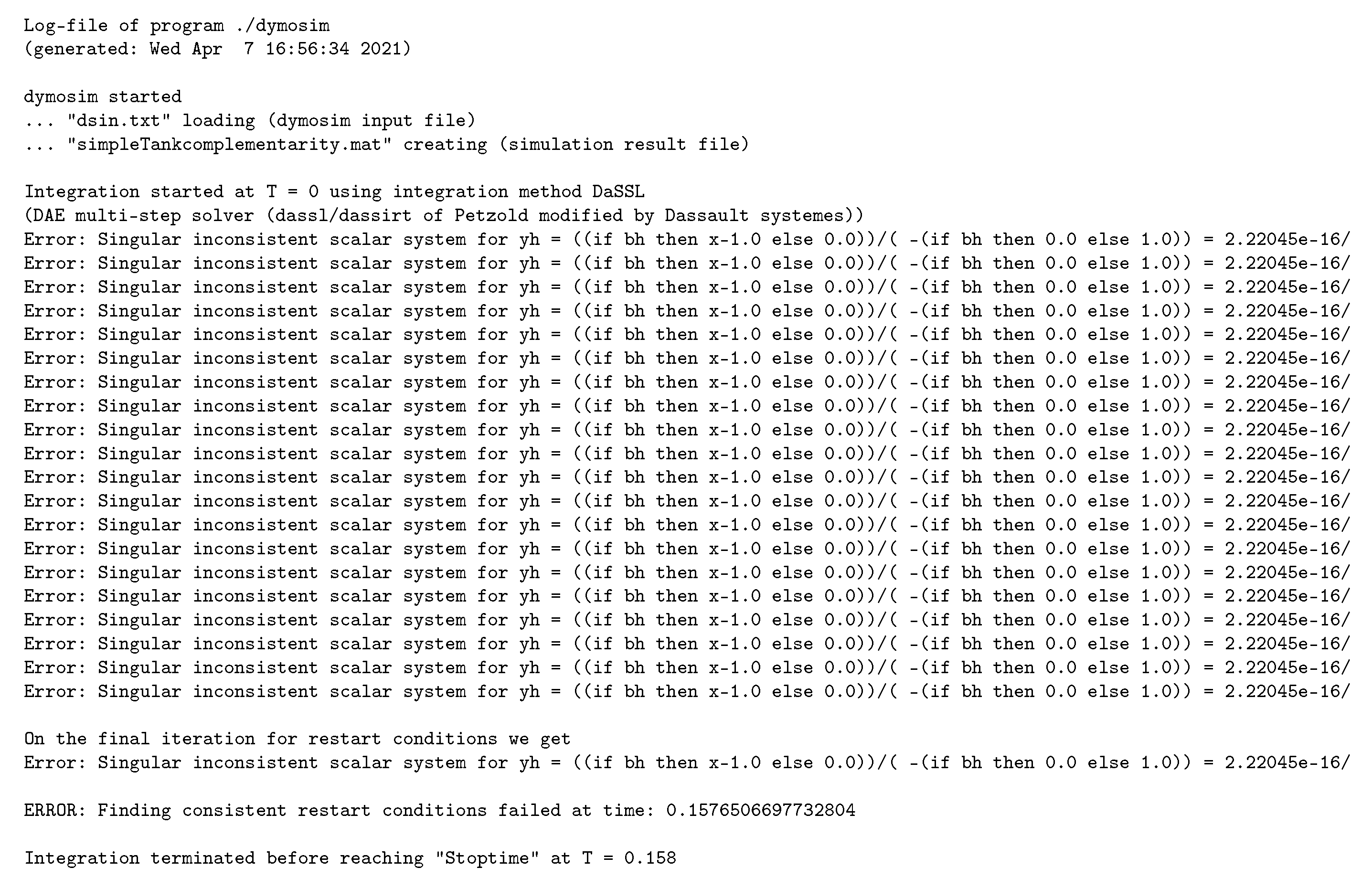
This model fails to simulate properly with both OpenModelica 1.17.0 and Dymola 2021; Figure 5 shows the output of Dymola 2021.
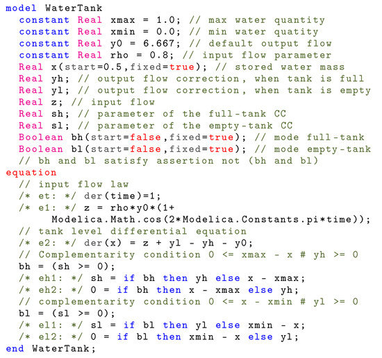
Figure 4.
Modelica model of the Water Tank system. Comments of the form /* id: */ define the equation labels that appear in the dependency graphs in Figure 6 and Figure 7.
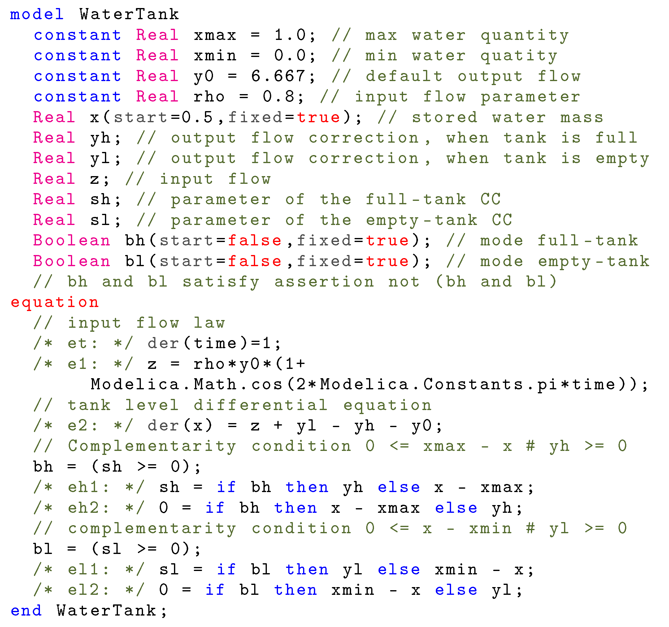
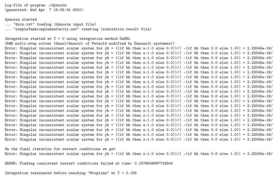
Figure 5.
Simulation of the Water Tank system with Dymola 2021, failing with a division by zero exception.
Figure 5.
Simulation of the Water Tank system with Dymola 2021, failing with a division by zero exception.
Once again, the root cause of this behavior is that state-of-the-art Modelica tools perform an approximate structural analysis, disregarding the fact that the structure of the system is mode-dependent. For the Water Tank model, this analysis results in the DG shown in Figure 6.
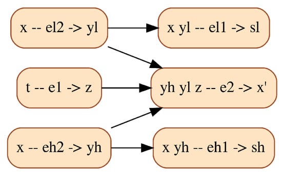
Figure 6.
DG resulting from the approximate structural analysis of the Water Tank model. Vertices are labeled following the same rules as for Figure 2. Edges express causal dependencies, meaning that a block can be solved only after all its predecessors have been solved.
Figure 6.
DG resulting from the approximate structural analysis of the Water Tank model. Vertices are labeled following the same rules as for Figure 2. Edges express causal dependencies, meaning that a block can be solved only after all its predecessors have been solved.
In this decomposition, equation eh2 has to be solved for the variable yh. When performing the pivoting of this equation, mode dependencies have to be taken into account again. Equation eh reads:
which can be rewritten as an equation of the form 0 = a yh + b where a and b are mode-dependent:
Unknown yh can finally be isolated:
A problem is then bound to occur at runtime when Boolean variable bh is true. As a matter of fact, Equation (1) is exactly the equation responsible for the division by zero exception shown in Figure 5, which occurs at the initial time, when bh is true.
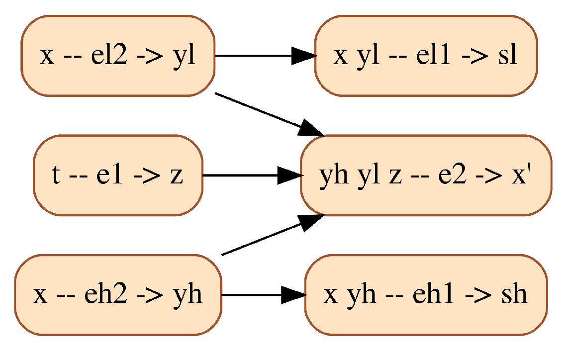
For comparison, the CDG resulting from the multimode structural analysis of this model is shown in Figure 7. Remark that equation eh2 is no longer used to compute yh in all modes, but only when bh is false, thus preventing the runtime error explained above.
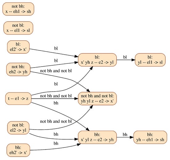
Figure 7.
CDG resulting from the multimode structural analysis of the Water Tank model. Vertices are labeled following the same rules as for Figure 2. Edges express causal dependencies, meaning that a block can be solved only after all its predecessors have been solved. They are labeled by Boolean conditions, characterizing the modes in which the dependency applies.
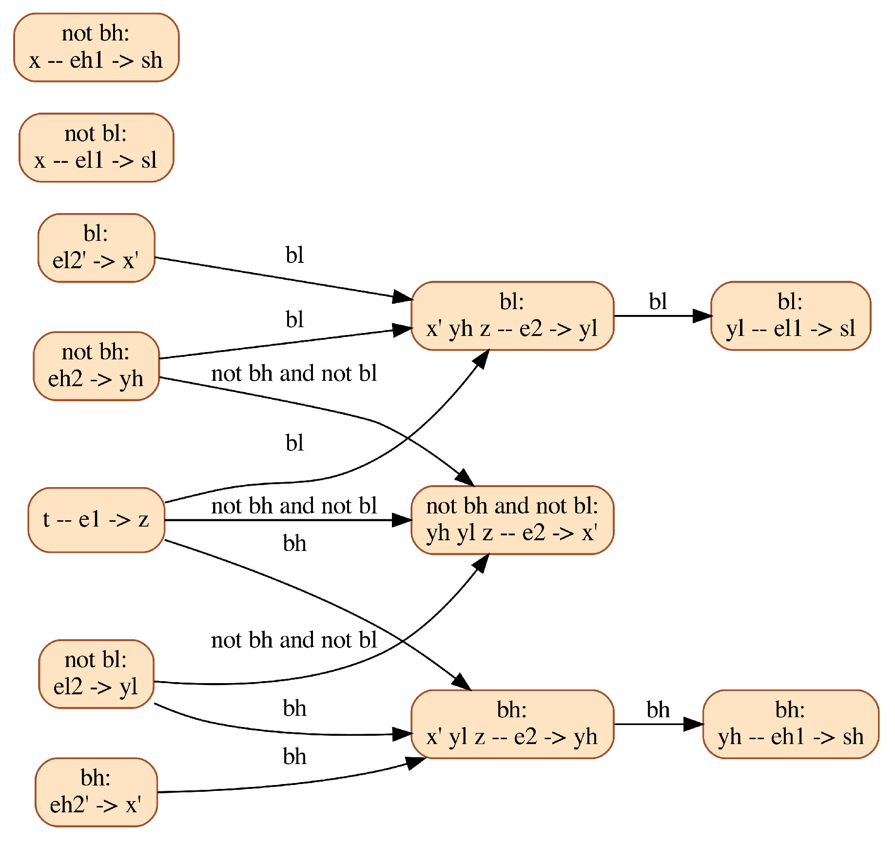
Moreover, notice that the orders of differentiation of the equations of this system are mode-dependent. For instance, equation el2 is used differentiated, to compute the derivative of x, when bl is true, while it is kept undifferentiated, to compute yl, when bl is false. A genuine multimode Modelica compiler must be able to handle models with variable (mode-dependent) differentiation index.
2.3. A Clutch Model
The clutch depicted in Figure 8 is an idealized clutch interconnecting two rotating shafts.
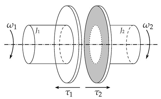
Figure 8.
An ideal clutch with two shafts.
It is assumed that this system is closed, meaning that the two shafts are not connected to anything else, whence the corresponding model:
In model (2), the dynamics of each shaft i is described by ODE for some, yet unspecified, function , where is the angular velocity and is the torque applied to shaft i. Depending on the value of the input Boolean variable , the clutch is either engaged () or released ().
When the clutch is released, the two shafts rotate freely: no torque is applied to them (). When the clutch is engaged, it ensures a perfect join between the two shafts, forcing them to have the same angular velocity () and opposite torques (). When , equations are active and equations are disabled, and vice-versa when . The model yields an ODE system when the clutch is released, and a DAE system of index 1 when the clutch is engaged.
If the clutch is initially released, then, at the instant of contact, the relative speed of the two rotating shafts jumps to zero; hence, an impulse is expected on the torques.
- The clutch in Modelica:
Figure 9 details the Modelica model of the Ideal Clutch system. It is a faithful translation in the Modelica language of the two-mode DAE (2), except that the two differential equations have been linearized. Moreover, the trajectory of the input guard (here called g) has been fully specified: it takes the value between and and otherwise.
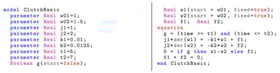
Figure 9.
Modelica code for the idealized clutch.
This model is deemed structurally nonsingular by both OpenModelica 1.17.0 and Dymola 2021. However, none of these tools generates the correct simulation code from this model. Indeed, simulations fail precisely at the instant when the clutch switches from the uncoupled mode (g=false) to the coupled one (g=true). This is evidenced by a division by zero exception, as shown in Figure 10.

Figure 10.
Division by zero exceptions with Dymola 2021 (top) and OpenModelica 1.17.0 (bottom) occurring when simulating the Ideal Clutch Modelica model.
As with the previous examples, the approximate structural analysis performed by the tools yields incorrect simulation code. In this case, it finds that the second-to-last equation of the model has to be solved for unknown f1 in all modes. Isolating this unknown in the equation, in a way similar to what was shown for the Water Tank model above, one gets:
Equation (3) is responsible for the division by zero exception shown in Figure 10, which occurs as soon as g becomes true.
However, addressing this shortcoming of current Modelica tools would still not guarantee the correctness of the simulation. To better understand the remaining difficulties, we provide the CDG of the clutch model in Figure 11.
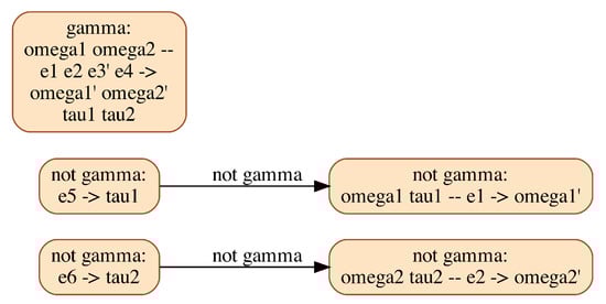
Figure 11.
CDG resulting from the multimode structural analysis of the Clutch model.
This graph shows that the mode-dependent equation has to be differentiated once. Equation reads ; its activation, at the instant when switches from to , forces and to instantaneously take equal values from (a priori) distinct values: choosing a common restart value for these variables is a difficult issue. Moreover, state variables and are impulsive, so their value at the instant of mode change cannot be set. A genuine multimode Modelica compiler must be able to handle (possibly impulsive) restart conditions at mode changes, including for models with variable index.
3. A Proposal for a Variable Dimension Extension of the Modelica Language
A model of a possibly faulty transmission line is used to give flesh to a proposed extension of the Modelica language, enabling variable structure and variable dimension systems. It is a lumped model, consisting of the series interconnection of N instances of the same Modelica model, derived from an equivalent electrical circuit of the transmission line element shown in Figure 12. The element has three possible modes of operation, depending on the states of the two switches:

Figure 12.
Equivalent electrical circuit of a faulty transmission line element.
- Nominal mode, when the open switch is closed, and the short switch is open (in this mode, nominal behavior is expected, while the other two modes are related to faults);
- Open circuit mode, where both the open and short switches are open;
- Short circuit mode, where both the open and short switches are closed.
The configuration where the open switch is open and the short switch is closed does not correspond to a legal mode of the model. The corresponding Modelica model is given by Figure 13. Note that equations v=0 and j=0 appear in this model only for the sake of defining the dynamics of variable v when in open circuit mode (Boolean open is true), and of variable j when in short circuit mode (Boolean short is true).
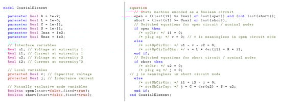
Figure 13.
Modelica model of the faulty transmission line element.
These equations can be regarded as plug equations: they are equations that result in the assignment of variables to a default value, with the sole purpose of keeping the same number of variables and equations in all modes. Such equations would be made unnecessary if variable v was defined only when open is false, and variable j was defined only when short is false. This would be achieved by placing the corresponding variable declarations in if-then-else conditional statements, as shown in Figure 14. Although Modelica does not allow for this, at the time of writing of this paper, this could be a simple and handy extension of the Modelica language, that would enable the support of genuine variable dimension systems.
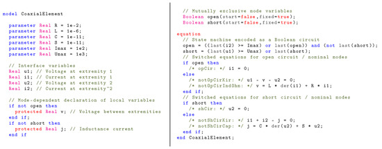
Figure 14.
Variable dimension model of the faulty transmission line element.
The lumped model of the transmission line is given in Figure 15. The execution of this model by current Modelica tools such as Dymola and OpenModelica yields an exception at runtime. The analysis of this model, with N set to 1, by the IsamDAE tool, yields the conditional dependency graph shown in Figure 16, which sheds light into the cause of this behavior: the set of leading variables of this model depends on the mode, which current industrial-strength tools fail to handle in all generality. For instance, when in mode element[1].open, element[1].i1 is computed by solving equation element[1].opCir; in the other two modes, it is its first order derivative that is computed by solving equation element[1].notOpCirIndOhm.
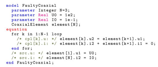
Figure 15.
Assembly of N instances of transmission line elements.
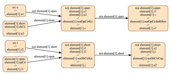
Figure 16.
CDG resulting from the multimode structural analysis of the FaultyCoaxial model with . This graph shows, in particular, that it is a variable structure system, where the set of leading variables depend on the modes.
4. Algorithmic Building Blocks
Our approach to a truly multimode compilation of the Modelica language requires a number of new algorithms. It turns out that such algorithms are easily built on top of a few basic building blocks. This is an important observation since it allowed us to focus on the effectiveness and ability to scale up for these building blocks only—the latter issue is mentioned in Section 4.1 and further detailed in Section 5. In this section, we present these building blocks in detail, namely:
- A concise representation of the mode-dependent structure of multimode systems, Section 4.1;
- A multimode extension of the Dulmage–Mendelsohn decomposition, Section 4.2;
- A multimode extension of Pryce’s -method, Section 4.3.
In the rest of this article, only models with a finite number of modes are addressed; more specifically, we assume that models are written using mode variables of type Boolean only; denotes the Boolean set, with elements (the “false” constant) and (the “true” constant).
4.1. Dual Representation of Multimode Systems
The core idea behind our multimode extension of the structural analysis chain is the introduction of a “dual” representation of the mode-dependent structure of a multimode system. As an illustration, instead of describing, for each mode, the set of active equations, this representation handles, for each equation, a propositional formula describing the subset of modes in which this equation is active. The whole structural information of the system is stored in a similar way, so that the structural analysis of the model can then be performed in an “all-modes-at-once” fashion, without enumerating the modes.
This dual encoding of the structure of a system consists of the set of Boolean functions [22,23] listed below. For efficiency purposes, these functions can be represented by means of Binary Decision Diagrams (BDD); in our implementation in the IsamDAE tool (see Section 6), we use the Reduced-Ordered variant (ROBDD) introduced by Bryant [24].
The predicates guarding both the equations and variables are abstracted as independent Boolean variables grouped in a set M. The set of modes, that can be denoted by , is then the set of valuations of these variables. Information about the relationship between the actual predicates can be preserved under the form of a propositional formula, called invariant in the sequel.
Each equation, variable and edge is associated with its own Boolean variable; the sets of Boolean variables for equations, variables and edges are denoted by I, J and E, respectively. Every edge of the adjacency graph is weighted according to the highest order of differentiation of the variable appearing in the equation. The mode-dependent values of these weights, which extend the definition of the given in Section 4.3, are stored as a function of both the mode and edge Boolean variables.
Table 1 describes the functions that encode the structure of an mDAE. Note that a little-endian variable-length binary encoding is used to represent integer functions.

Table 1.
Functions generated from parsing the model.
Constraint on the possible valuations of Boolean mode variables describes the invariant of the system; a valuation is a valid mode (This notion of validity of a mode is a structural property, independent from the dynamical property of reachability of a mode: a mode might be valid but unreachable) if , an invalid mode if . The set of valid modes is then denoted by , where one naturally has .
The guards on the equations (resp. variables, edges) are described by function (resp., , ).
Several functions are also defined for later use in our algorithms: functions and , respectively, return the equation and variable associated to a given edge; functions and , respectively, return the set of edges incident to a given equation and variable.
In order to turn the core idea behind our approach into an efficient implementation, it is of paramount importance that this dual data structure is manipulated at all stages of structural analysis. As a result, the multimode extensions of existing algorithms, detailed in Section 4.2 and Section 4.3 below, are all written in terms of Boolean operations on functions, esspecially those directly generated from parsing the model (see Table 1).
4.2. A Multimode Dulmage–Mendelsohn Decomposition
The Dulmage–Mendelsohn (DM) algorithm, introduced in [25], is a canonical decomposition of the set of vertices of a bipartite graph that is commonly used for solving systems of algebraic equations. This decomposition partitions set I (respectively, set J) into three subsets , and (resp., , and ), so that the following properties are satisfied:
- , , ;
- a maximum matching of G can only join a vertex of to a vertex of , a vertex of to a vertex of , a vertex of to a vertex of ;
- a maximum matching of G can always be restricted to a perfect matching between and ;
- there is no edge between a vertex in and a vertex in ;
- there is no edge between a vertex in and a vertex in .
The DM decomposition can be applied to the adjacency graph of a system S of algebraic equations, where each vertex in I represents an equation, each vertex in J represents a variable, and an edge is in E if and only if variable j occurs in equation i. The set of equations is then partitioned into three subsystems: we say that is the underdetermined part of S, is its square (or well-determined) part, and is its overdetermined part; the corresponding subsets of J are the subsets of their dependent variables.
In order to write down the incidence matrix of system S, one has to fix a total order on equations and a total order on variables: these orders yield the indexing of rows and columns of the incidence matrix. The following propositions are then equivalent:
- the total orders and are consistent with the DM decomposition, in the sense that the following conditions are met:
- (i)
- , and
- (ii)
- ;
- the incidence matrix of S, with respect to order on equations and order on variables, is in upper block-triangular form.
An efficient algorithm for computing the DM decomposition of sparse systems was published by Pothen and Fan in [15]. A maximum matching of the system’s adjacency graph is required as an input. An alternating path (with respect to the matching ) is a path whose edges belong alternatively to and . Let (respectively, ) be the set of unmatched equations (resp., unmatched variables). Then:
- and are the subsets of I and J (respectively) that are reachable via an alternating path from ;
- and are the subsets of I and J (respectively) that are reachable via an alternating path from ;
- and collect the remaining equations and variables.
This decomposition is independent of the choice of the maximum matching.
- Multimode extension:
Our multimode adaptation of the Dulmage–Mendelsohn algorithm is designed for algebraic systems of equations in which both equations and variables can be guarded by propositional formulas on mode variables, and where equations can contain if-then-else statements. It is based on the dual representation of the structure of the system introduced in Section 4.1 above. In particular, the functions encoding the structure are those given in Table 1, except for as one now deals with algebraic systems.
The choice of one maximum matching per mode is performed without enumerating the modes, thanks to computation steps similar to those that will be described in further detail in Section 4.3, for the solving of the so-called primal problem. For understanding our extension of the DM decomposition, one just needs to know that indicator functions are computed for each edge , indicating the modes in which the edge is part of the corresponding chosen maximum matchings.
For each equation , we define three functions , , whose final values will state the modes in which this equation belongs to the overdetermined, underdetermined and square subsystems, respectively. Each is initialized so that it encodes the set of modes in which equation i is unmatched, that is:
while functions and are initialized to , the false constant.
In a similar fashion, three functions , , are defined for each variable . Functions are initialized so as to represent the sets of modes in which the considered variables are unmatched, while functions and are initialized to .
The so-called propagation steps that follow consist in exploring alternating paths from the “overdetermined sets” , (respectively, the “underdetermined sets” , ) and updating the corresponding functions until a fixpoint is reached.
For the underdetermined part, one can observe that, in order to explore alternating paths, only edges outside of can be followed from vertices in , while only edges of can be followed from vertices in . The propagation steps can then be written as follows:
These steps are repeated until a fixpoint is reached.
Note that the second assignment in (5) does not explicitly involve function as it was already involved in the computation of the maximum matchings, i.e., the implication holds for every .
In a similar fashion, the propagation steps for the underdetermined part are given by:
Finally, once the functions representing the mode-dependent over- and underdetermined parts were computed, the determined parts are made of the equations and variables that are not part of the other two parts of the decomposition:
The correctness of the resulting decomposition is ensured by design, as the evaluation of the above formulas for any valid mode exactly yields the original algorithm by Pothen and Fan [15]. The computed functions are functions of the mode variables only. This ensures both the compactness of the representation of the multimode DM decomposition and its computational tractability. Finally, note that it is sufficient to append conjunctions with a fixed function to specify a subset of modes in which the DM decomposition must be computed; all modes for which this function returns are then essentially ignored.
4.3. A Multimode Extension of Pryce’s -Method
Albeit less renowned than the Pantelides method [3], Pryce’s -method [4] is an efficient structural analysis method for DAEs, whose equivalence to the Pantelides method has been proven by the author. This method consists in solving two successive problems, denoted by primal and dual, relying on the Σ-matrix, or signature matrix, of a DAE system.
Let F be a square DAE system of size n, with I (respectively, J) denoting its set of equations (resp., dependent variables); we generically denote by either i or an equation of this system, and by j or a variable of this system. Each equation only involves a finite number of variables and their successive time derivatives, as well as the time variable t itself.
The -matrix of this system is given by:
where is the maximal order of differentiation of variable in equation , or if this variable does not appear in the equation. The same structural information can be represented as a weighted adjacency graph, a bipartite graph whose left nodes represent equations and right nodes represent variables; in this graph, each edge represents the occurrence of a variable in an equation, and is weighted by the value of the corresponding . Set E collects all edges of this graph, which corresponds to all pairs such that .
The primal problem consists in finding a maximum-weight transversal in matrix or, equivalently, a maximum-weight perfect matching (MWPM) in the weighted adjacency graph. The underlying linear problem can be written as follows:
This is actually an assignment problem for the solving of which several standard algorithms exist.
The dual problem consists in finding a specific solution to a given linear programming problem (LP), defined as the dual of the aforementioned assignment problem. Every solution of the LP is such that system , obtained by keeping the -th time derivative of every equation , is a structurally nonsingular system whose leading variables are the -th time derivatives of each variable ; the dual problem consists in finding the (component-wise) smallest nonnegative solution of this LP, whose existence and uniqueness are guaranteed provided that the primal problem has at least one solution (Section 3.2 of [4]).
In practice, the dual problem is solved by means of a fixpoint iteration (FPI) that makes use of the MWPM found as a solution to the primal problem, described by the set of tuples :
- Initialize to the zero vector.
- For every ,
- For every ,
- Repeat Steps 2 and 3 until convergence is reached.
- Multimode extension:
In the multimode setting, the primal problem consists in finding, for every mode , a solution to the following linear program:
where the fresh condition on edges is introduced in order to take into account the mode dependency of edges. Our initial approach for solving this problem without mode enumeration, as described in [6], consisted in computing several functions one after the other:
- describes all perfect matchings in all valid modes; it can be computed as the conjunction of several functions, representing the uniqueness constraints on both equations and variables, as well as the constraint that only edges that are active in a given mode can be part of a matching in this mode.
- describes all MWPMs in all valid modes; it can be computed by pruning out from X every matching whose weight is not maximal, thanks to the use of a weight function computed from function .
- restricts S by selecting one and only one MWPM per valid mode; it can be efficiently computed by an inductive algorithm on the BDD encoding function S.
- For convenience, a function is computed for every edge , indicating the valid modes in which edge e is part of the chosen MWPM.
Section 5 introduces an algorithm that alleviates the need for this computation chain and improves the associated computational times by several orders of magnitude.
Finally, the FPI algorithm used for solving the dual problem has to be adapted in our setting, so that it computes functions (for every ) and (for every ). For simplicity, a (resp. ) is set to 0 in those modes in which equation (resp. variable ) is disabled; in the end, functions and indicate the modes in which each and each has to be considered so that the choice of this default value is harmless—the value 0 actually helps keep BDD representations concise. Note, however, that the parametrized FPI has to explicitly take into account the conditions enforced by functions , and .
Using a parametrized max function, as well as arithmetic operations and a parametrized if-then-else operator, the parametrized FPI reads as follows:
- Initialize to the zero function.
- For every ,
- For every ,
- Repeat Steps 2 and 3 until convergence is reached.
By design, the method detailed hereinabove returns functions of the mode variables that, once evaluated for a particular mode, yield the same results as the single-mode structural analysis of the resulting DAE.
5. Addressing the Scalability Challenge with the CoSTreD Method
As shown in Section 4.3 above, the first step in Pryce’s -method is the solving of the primal problem, which consists in finding an MWPM (maximum-weight perfect matching) in the weighted adjacency graph of the considered DAE system. The multimode extension of the primal problem aims at computing functions of the modes representing the choice of one MWPM per mode; this information may be encoded as, either a single function , or a set of functions .
The approach presented in Section 4.3 for solving the multimode primal problem alleviates the need for enumerating the modes of a model. Nevertheless, it still proved to yield very high computation times. The root cause of this issue is the need for computing several functions of large numbers of variables and performing sophisticated operations on those. This section introduces a decompositional method for solving the primal problem introduced in Section 4.3, and illustrates it on the transmission line model from Section 3.
We reformulate the primal problem by using the fact that both the Boolean constraints and the objective function of this problem can be uniformly expressed as weighted constraints in the generic context of the weighted Constraint Satisfiability Problem [26] (wCSP). Quite importantly, we show that the overall structure of the system (in terms of interconnections between modules) is preserved by this transformation. In other words, sparse DAE models yield sparse constraint systems, on which a decompositional approach can prove highly effective.
In this section, the concept of wCSP is extended to multimode wCSP, or mwCSP. From a mathematical point of view, solving an mwCSP amounts to solving a wCSP for every valuation of the mode variables. In practice, we use symbolic representation to solve the mwCSP as a whole, without explicitly enumerating these valuations. Remark that we use the term multimode for the sake of consistency with multimode DAE systems, but it should be clear that the notion of mode exactly corresponds to the notion of parameter in mathematical programming.
The core of this section is about how the Constraint System Tree Decomposition (CoSTreD) method, detailed in the research report [27], is used for solving this problem; this amounts to a specific implementation of the CoSTreD method for the optimization of weighted constraints.
It is worth noting, though, that the approach presented in the research report can be applied in full genericity to solve many constraint-stated optimization problems. The experimental results obtained with the IsamDAE tool (see Section 6) heavily rely on the implementation of the CoSTreD method, not only for solving Pryce’s primal problem, but also for the multimode Dulmage–Mendelsohn decomposition (see Section 4.2) and the structural analysis of consistent initialization (Section 7). Demonstrating the efficiency of CoSTreD on use cases other than these is a work in progress.
Name disambiguation: In what follows, we will be distinguishing between the propositional variables, which are Boolean variables involved in the mwCSP; the mode variables of the model, that are used as mode variables in the mwCSP; and the model variables, which are just the real variables from the source model.
5.1. Related Work
The CoSTreD method is a dynamic programming approach, which exploits a “good” tree decomposition [28] of a system. It breaks down the resolution of large, yet sparse, problems into sets of smaller, thus simpler, problems. Variations of this method have been rediscovered many times in the history of computer science, under various names: message passing in factor graphs, belief propagation in belief networks, arc consistency in constraint networks [29], etc. Message-passing techniques have been extensively used in statistics, signal processing and constraint programming; however, as far as we know, their multimode extension had not been considered so far.
Various sources confirm the use of symbolic representation to efficiently deal with local problems, in the context of message passing methods. However, the use of Binary Decision Diagrams (BDDs) within this setting is quite original, since we can only cite the work of Lande and Swoboda [30] for the case of 0-1 ILP (Integer Linear Programming).
5.2. Constraint Dependencies Follow Component Interconnections
Because of the component-based design of large-scale Modelica models, such models are typically sparse, in that each component only interacts with a few other components. Hence, each model variable is only used in a few equations and each equation only involves a few model variables. Therefore, the resulting flat Modelica model (following the procedure described in Chapter 5 of the Modelica Language Specification [18]) is sparse.
To formalize the notion of sparsity, in the context of wCSP and mwCSP, we use the notion of primal graph of a constraint system, that is, the undirected graph where two variables are related if and only if they appear in a common constraint. We emphasize that the notion of the primal graph should not be confused with the weighted adjacency graph used in the statement of Pryce’s primal problem.
Recall that the multimode primal problem consists in finding an MWPM of the weighted adjacency graph, in each valid mode of the model. System (10), Page (16), is an mwCSP encoding of this problem, where one propositional variable is associated to each edge of the weighted adjacency graph (that is, each pair such that model variable j occurs in equation i), and the mode variables from the original model are kept as mode variables of the mwCSP. Hence, the corresponding vertices in the primal graph are adjacent, if and only if the corresponding edges share a common model variable or a common equation. As a result, the sparsity of the original model yields the sparsity of the mwCSP that represents the primal problem.
A particular case is that of chain-shaped systems; the faulty transmission line model from Section 3 is a typical example of such systems. Its primal graph, given in Figure 17, clearly illustrates the fact that the overall structure of the original model, made of small components interconnected by a few variables, is preserved in the primal graph.
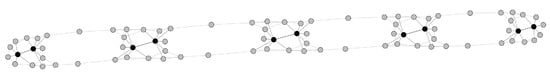
Figure 17.
Primal graph of the faulty transmission line model for components. Grey vertices represent propositional (edge) variables, while black vertices represent mode variables.
5.3. Generic Single-Mode Formulation
Optimization problems are typically made of an objective function to be maximized, and a set of Boolean constraints that have to be met. In our setting, we will instead deal with two sets of “constraints”, as the objective function will implicitly be declared as a set of reward functions whose sum has to be maximized. Let us introduce these sets and exemplify them on the (single-mode) primal problem as given in System (9), Page (15):
- is a set of reward functions on set X; for any valuation , we denote .
- This set of functions expresses the quantity to be maximized. In the primal problem, the objective function given by (9a) is ; it can be kept as a monolithic constraint (in which case it would be the only element in ), or decomposed as the set of constraints for all . By definition of , both approaches yield the same objective function, but the second one ensures a better sparsity of the primal graph of the constraint system.
- is a set of Boolean constraints on the set X of propositional variables; for any valuation , we denote .
- This set of constraints is used to filter out valuations that do not meet the given criteria. In the primal problem, where the propositional variables are the ’s, set collects all constraints (9b) and (9c). Each of these constraints can be seen as a Boolean function that, given a valuation , returns if the constraint holds for , otherwise. As a result, returns if and only if encodes a perfect matching.
Notation is used to denote the whole optimization problem, made up of constraints and reward functions . Then, denoting , we define the maximal weight reachable by assuming as:
In particular, this maximal weight is equal to if and only if the set of Boolean constraints is unsatisfiable:
For later convenience, we define as the characteristic function of the set of maximal weight solutions:
5.4. Generic Multimode Formulation
In order to extend the definitions above, one has to be aware that a solution of an mwCSP is itself a function of the mode variables. As we shall see, a direct consequence is that mode variables have to be handled in a different way than the other variables; in other words, propositional variables and mode variables are not equal citizens. Therefore, we explicitly distinguish propositional variables (edge variables in the example of the primal problem) from mode variables , as we did in System (10).
The above definitions and properties are extended to a multimode setting as follows:
- a multimode Boolean constraint is of the form ;
- a multimode reward function is of the form ;
- the (mode-dependent) maximal weight is defined asand the relationship between this and the unsatisfiability of the set of Boolean constraints now reads
- finally, is similarly extended as
5.5. Unified Formulation
For convenience, we want to deal with Boolean constraints and reward functions by unifying them into a single concept. For this reason, the notion of weighted constraints is defined as follows:
- for each Boolean constraint , we introduce a weighted constraint ;
- for each reward function , we introduce a weighted constraint by just extending the co-domain with .
We can then define an addition law + on weighted constraints, by using the classical addition law on naturals, extended with as an absorbing element, that is: . It is worth noting that, for any weighted constraints and , is itself a weighted constraint.
The unified optimization problem is defined by:
- two sets of variables X and M, with the same meaning as above, and
- a set of weighted constraints , whose semantics is defined byRemark that the semantics of a constraint system is a constraint itself. In many cases, this allows us to reason on constraints, instead of constraint systems.
Weighted constraints can, in turn, be transformed back into Boolean constraints and reward functions by considering both the Boolean and weighted projection operators:
Hence, we have . In what follows, the Boolean projection will be of particular interest when reasoning in terms of sets of solutions. In our unified framework, we actually consider as a subset of , by identifying with (the constant true) and 0 with (the constant false), in accordance with the definition of the Bool operator.
For any multimode weighted constraint , we can now define and as follows:
The definition of the operator relies on the fact that is identified as a subset of : this enables us to handle Boolean constraints in an explicit way, while still being able to use the addition law + on all weighted constraints indifferently.
Note that the max and operators satisfy a weak compositional property that is required for our approach: for two constraints and , where and are disjoint sets, the constraint is such that
(up to an embedding of and in by adding useless variables in their respective supports). No such property, however, holds in general for constraints whose supports are overlapping.
We define the optimizing semantics of a constraint (or constraint system) f as the pair
The equivalence of two constraints is then defined by the equality between their respective optimizing semantics:
As we shall see, the compositional solving of a constraint system is made difficult by the fact that this equivalence is not congruent for the addition law +, that is:
Finally, we introduce a multimode notion of maximal weight solution.
- First, we define a multimode valuation as a function , that is, a function that, for each mode, returns either a valuation or . Given a multimode constraint , we define as follows:
- Then, we say that a multimode valuation V is a multimode solution ifFor the solving of the multimode primal problem, this function returns for a given mode if no perfect matching exists in this mode; otherwise, it returns the encoding of a perfect matching.
- Finally, we say that a multimode valuation V is a maximal weight multimode solution ifOn may notice that V is, in particular, a multimode solution. By convention, maximal weight multimode solutions are denoted by . In particular, in the context of the multimode primal problem, is a function which, for each mode , returns an encoding of an MWPM if at least one perfect matching exists, otherwise.
In the remainder of this section, we assume without loss of generality that the primal graph is connected: whenever it is not, as the weak compositional property given by Equation (21) is satisfied, one can split the problem across the connected components, then aggregate their solutions to obtain a solution to the original problem.
5.6. Single-Mode Decompositional Approach
In the above, we introduced mwCSP and a unified formulation where Boolean constraints and reward functions are cast into a unique notion of weighted constraints. Now that the stage is fully set up, we may delve into the decompositional approach that grounds the CoSTreD method. For the sake of clarity, CoSTreD is first introduced on an illustrative example, then developed in all generality for wCSP, that is, without mode variables. Section 5.7 deals with its extension to mwCSP.
- Illustrative example
This example shows how the CoSTreD method would handle the wCSP resulting from the transmission line model introduced in Section 3, with , and where all lump elements are forced in a nominal mode so that no mode variables appear in the constraint system. Formal definitions and algorithms will be given in the remainder of this section.
Figure 18 shows the primal graph of the constraint system under study, where the grey vertices represent the propositional (edge) variables, along with a representation of a tree decomposition for this system.
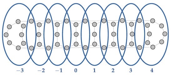
Figure 18.
Primal graph and tree decomposition of the transmission line model for lump elements, forced in nominal mode. The blue bubbles represent the nodes of the tree decomposition; here, they are indexed from left to right, with node 0 acting as the root of the tree.
The blue bubbles represent the nodes of this decomposition; they are chosen so that each clique of the primal graph is included in at least one node. This ensures that, for each constraint of the wCSP under study, its set of variables in included in at least one node of the tree decomposition, so that the nodes define a partitioning of the constraint system into subsystems. Each of these subsystems are, in turn, regarded as a single constraint, as per Equation (17).
Edges of the tree decomposition connect nodes that share variables. Hence, the tree decomposition of Figure 18 is actually a chain of 8 nodes, each one associated with a single constraint. Each node could be chosen as the root of the tree; here, node 0 is picked as root.
The CoSTreD method solves the wCSP using a process akin to message passing [29], and based on this decomposition. Messages are propagated, first from the leaves to the root (“forward”), then back to the leaves (“backward”) (If we regard the tree decomposition as an in-tree, that is, a directed tree with all its edges pointing towards the root, then the “forward” operations follow the directed edges, while the “backward” operations proceed in the reverse order); these successive stages are, respectively, called Forward Reduction and Back-Selection. On the example of Figure 18, they act as follows:
- Forward Reduction: Start from node , one of the leaves of the rooted tree. The constraint sitting in it undergoes two operations:
- Projection: Variables that only belong to node are eliminated in such a way that all necessary information about the maximal possible weight is preserved. This information is passed to node and combined with the constraint sitting in that node.
- Co-Projection: The original weighted constraint sitting in node is turned into a Boolean constraint describing conditions under which a valuation of the variables can be a maximal weight solution of the wCSP. To our knowledge, this operation was not introduced in message passing techniques; it is instrumental to the second stage of the method, the Back-Selection (see below).
This process is repeated toward the root, on node , then on node . In parallel, the other branch is handled in a similar fashion, from node 4 to node 1; the final constraint sitting in node 0, the root of the tree decomposition, combines the original weighted constraint sitting in node 0 with the constraints received from nodes and 1.Solving this constraint can actually be performed by applying the projection and co-projection operators. The former yields the global maximal weight, while the latter provides a Boolean constraint on the set of maximal weight solutions; any valuation of the variables of node 0 that satisfies this constraint is a partial solution, meaning that it can be extended into a maximal weight solution of the original wCSP. - Back-Selection: The Boolean constraints sitting in the nodes of the tree decomposition are the results of the co-projections performed during the Forward Reduction. As we shall see in the rest of this section, the design of the CoSTreD method ensures two important properties: any valuation of the variables that satisfy all these constraints at once is a maximal weight solution, and a partial solution can always be extended into such a solution.To do so, the Boolean constraints sitting in the nodes are taken into account in a top-down fashion, that is, from the root of the tree to its leaves. This extends, in successive steps, the partial solution computed in node 0 into a global maximal weight solution of the original wCSP.
The CoSTreD method, like message passing methods, only requires the solving of local subsystems, involving a (possibly small) set of variables contained in a single node. However, it has the unique asset that maximal weight solutions can be rebuilt “in one go” during the Back-Selection process.
The method is the end result of a very careful design process. The main difficulty consists in ensuring that the optimizing semantics (see Equation (22)) of the original constraint system is preserved by the Forward Reduction, by having it unchanged at every step of this process. In other words, every Forward Reduction step must preserve, not only the maximal weight of a solution, but also the actual set of maximal weight solutions.
This property is a difficult one to ensure, because of the lack of a congruence property for the semantics of a constraint system; that is, a constraint cannot, in general, be replaced with an equivalent one without changing the overall semantics. To overcome this difficulty, the definitions of the projection and co-projection operators had to be carefully crafted.
In what follows, the method described in the example above is formally defined, and important properties are given. These properties lead to the so-called Core Semantics Preservation theorem (Theorem 1), which guarantees that optimizing semantics are preserved by each Forward Reduction step. This makes it possible to prove the preservation of semantics by the Forward Reduction process, given by Theorem 2, which concludes this section.
- Constraint System Tree Decomposition
The CoSTreD method is based upon the a priori selection of a tree decomposition [28] of the (weighted) constraint system. A tree decomposition
satisfies the following two axioms:
- Nodes are sets of Boolean variables of the constraint system such that, for each constraint f of the system, its support is included in at least one node in B;
- The set of edges forms an undirected spanning tree on B and is such that, for every Boolean variable x, the set of nodes containing x is connected.
Tree decompositions are not, in general, a partitioning of the set of Boolean variables.
Computing an optimal tree decomposition of a constraint system is an untractable problem that is not considered therein. A “good” tree decomposition should consist of nodes with few Boolean variables. Several metrics exist in the literature to quantify tree decomposition, e.g., treewidth [28].
We assume that we are given a tree decomposition, and that each weighted constraint f is mapped to a node of the decomposition, in such a way that the support of the constraint is included in the corresponding node . This yields a partitioning of the constraints. For convenience, constraints mapped to the same node are summed into a single constraint. In particular, each node b of the decomposition is associated with a single constraint , such that . We define a Constraint System Tree Decomposition (or CSTD) as the tuple
Intuitively, some form of message passing can be implemented in a CSTD if an order is defined on the nodes of the tree decomposition: messages can then be sent following this orientation, in an iterative fashion, from the leaves to the root. Such an order can be obtained by first selecting a distinguished element of the tree decomposition D, which will be used as its root; we call a rooted tree decomposition. An orientation of is then induced by its root : we say that
The tuple is then called a rooted Constraint System Tree Decomposition, or rCSTD.
- Projection operators
A message passing-like operator can be defined for rCSTD, based upon a suitable form of projection.
Definition 1
(Existential Projection). Let f be a weighted constraint on a set of variables X. For any subset , the existential projection , where , is defined as follows:
To avoid unnecessary domain castings, it is assumed that is embedded back into by reintroducing variables in Y as useless variables.
In other words, is a constraint obtained from f by a specific “existential elimination” of the variables in Y, in such a way that all necessary information about the maximal weight is preserved: for any valuation , one has if and only if (i) there exists an extension of such that , and (ii) there exists no extension of , such that .
For the sake of simplicity, we also define the (projective) restriction of a constraint f to the set of variables Y as .
However, we want to keep track, not only of the maximal weight, but also of the corresponding maximal weight solutions, that is, valuations of the propositional variables that maximize the weight. In the context of the primal problem, one is not even interested in the maximal weight itself, but only in the maximal weight solutions, that is, the MWPM. The co-projection operator introduced below will be used to collect all local information necessary for reconstructing such solutions.
Definition 2
(Co-Projection). Let f be a weighted constraint on a set of variables X. For any subset , the co-projection is defined as follows:
The definition of co-projection mirrors that of the operator given in Section 5.3, in that acts as a characteristic function of the set of maximal weight solutions.
- Forward Reduction
The following properties are instrumental in establishing the correctness of message passing algorithms (These properties are actually axioms of the theory on which the generic method is based, as shown in [27]; it can be proved that they all hold in the context in which they are used here, because of the fact that is a totally ordered set on which the operator + is strictly monotonic, except for the absorbing () and neutral (0) elements):
Lemma 1.
Let f and g be two weighted constraints on the set X of propositional variables, and Y and Z be two disjoint subsets of X. The following properties hold, where ⊎ denotes the union of disjoint subsets:
- Assuming and , then
- If , then
- -
- -
These properties lead to the fact that for any weighted constraint f and any set of variables Y, one has
where ≡ was defined in (23). Property (28) enables us to define a message passing operation on rooted CSTD, called Forward Reduction. It is defined as follows:
Definition 3
(Forward Reduction). Let a rooted CSTD and a forward arc. The forward reduction operator is defined by:
Intuitively, the projection operator is used on so that the necessary information about the global maximal weight is propagated from s to d; by using this operation in an iterative fashion, up to the root of the tree decomposition, the maximal weight is computed in a compositional way “forward”.
As for the co-projection operator applied on , it makes it possible to only keep relevant information about the actual valuations that can yield this maximal weight: weighted constraint is reduced, during Forward Reduction, into a Boolean function that acts as a characteristic function of the set of maximal weight solutions. This information will later be used for reconstructing maximal weight solutions, if they actually exist, “backward”.
Note that Forward Reduction can be efficiently implemented using a symbolic algorithm such as the one described in our previous article [6].
We say that an arc is forward reduced in a rooted CSTD if . This leads to defining a forward reduced rCSTD as a rooted CSTD in which all arcs are forward reduced:
Definition 4
(Forward Reduced rCSTD). We say that a rooted CSTD is forward reduced if and only if:
Turning an rCSTD into a forward reduced rCSTD is performed by induction over the tree structure of the decomposition, by inductively propagating messages from the leaves to the root according to the orientation : this is called the Forward Reduction Process (or FRP).
If an inconsistent formula is detected at any point of the process, this means that the original constraint system is unsatisfiable (the maximal weight is ), so that the traversal of the tree decomposition can be stopped. Otherwise, one reaches the case where the original rCSTD has been transformed into a forward reduced rCSTD whose root node is satisfiable.
The FRP is performed in a linear number of reduction steps, and the fact that it always yields a forward reduced rCSTD can easily be proved by induction. However, the fact that the forward reduced rCSTD is equivalent to the original rCSTD is a major theoretical difficulty. The reason is that the equivalence of f and does not guarantee, in general, the equivalence of and , as stated in Equation (24). Preservation of semantics, in the sense of (23), by forward reduction is addressed later in this section.
- Back-Selection
After the FRP, all nodes of the tree decomposition, except for its root, only hold Boolean constraints (obtained by applications of the co-projection operator). The root node can then be decomposed into its projection and co-projection on the whole set X of propositional variables; the former yields the maximal weight, while the latter is, in turn, a Boolean constraint on the set of maximal weight solutions.
What distinguishes the CoSTreD method from standard message passing techniques is that a maximal weight solution can then be rebuilt in one go. For this purpose, the maximal weight sitting in the root node can simply be discarded; all nodes of the tree decomposition are now Boolean constraints. Starting from the root node, these constraints are taken into account in a top-down fashion, that is, via a simple depth-first traversal of the tree decomposition.
We call solution a valuation of the variables that satisfies all the Boolean constraints (nodes) at once; a partial solution is a partial valuation (that is, a valuation of a subset of the propositional variables) that can be extended into a solution. The process used for extending a partial solution into a solution is the Back-Selection, formally defined as follows (Algorithm 1).
| Algorithm 1: Back-Selection |
|
The back-selection process starts by computing a solution of the root constraint, which is a partial solution of the constraint system. It then extends this partial solution to its children, and so on. An important property to point out is that if a variable appears in two or more children of , then it appears in itself; as a result, applying Back-Selection to the children of does not pose any risk of “conflict” on variable valuations. This fact is key for the merging of valuations , …, at the very end of the algorithm, for creating a satisfying valuation of : either a variable appears in , in which case its valuation in is kept; or it appears, and is given a valuation, in a single . This “non-conflict” property is also used for proving the correctness of the algorithm in the research report [27].
- Correctness of the CoSTreD method
As stated above, it can easily be proved that the inductive application of Forward Reduction yields a forward-reduced rCSTD. As for the Back-Selection algorithm, its correctness is addressed above. Hence, the correctness of the CoSTreD method now lies in the preservation of semantics during the FRP.
Once again, this property is actually harder to prove than one may think at first glance, because of Equation (24) that states that ≡ is not a congruence for the binary operator +. One actually needs to focus on a single Forward Reduction step, on a given arc of the rCSTD, in the context of the whole FRP.
Figure 19 illustrates the general setting of the problem. In this figure:

Figure 19.
Illustration of the sets of constraints and variables involved in a Forward Reduction step. The names used are exactly those from Theorem 1.
- h denotes the constraint obtained by combining all constraints in the sub-tree rooted in s;
- f denotes the constraint to be processed by the Forward Reduction step;
- g denotes the constraint obtained by combining every other constraint.
The set X of propositional variables is partitioned according to this decomposition: A is the set of variables that are only involved in g, B is the set of variables common to the supports of g and f, C is the set of variables involved in f but not in g, and D is the set of variables that are involved in h but in neither g nor f.
It is important to note that, as the current Forward Reduction step is part of a whole “bottom-up” process, Forward Reduction was already performed on all the constraints from the sub-tree rooted in s. As a result, h is a Boolean constraint; this can actually be proved by induction. Furthermore, one can assume that : intuitively, this amounts to supposing that the Boolean constraints coming from the sub-tree rooted in s were correctly propagated during the previous steps of the FRP.
The above properties make it possible to prove the preservation of semantics during the current Forward Reduction step, which can be formalized by the following theorem:
Theorem 1
(Core Semantics Preservation). Let a 4-partition of X.
Let f, g, h three optimizing constraints such that:
- ;
- ;
- ;
- h is a Boolean constraint such that .
Let . One then has:
The proof of this statement, detailed in our research report [27], is performed by combining the properties stated above. Note that this result holds because of the very definitions of the projection and co-projection operators; the latter, in particular, was carefully designed so that the Forward Reduction operator preserves the set of maximal weight solutions.
Theorem 1 is then heavily used for proving the preservation of semantics during the whole process:
Theorem 2
(Forward Reduction Semantics Preservation). Let be a rooted CSTD, and be a forward arc. Assuming that , the sub-CSTD rooted in s, is forward reduced, the following properties hold:
- 1.
- ;
- 2.
- is forward reduced in ;
- 3.
- , the sub-CSTD of rooted in s, is forward reduced.
Theorem 2 guarantees the correctness of the FRP: the inductive application of the Forward Reduction operator on a rooted CSTD preserves the semantics of the original constraint system. After the FRP, the Boolean projection of the root node is forward consistent and equivalent to ; applying the Back-Selection algorithm on it yields a satisfying valuation of , that is, a maximal weight solution of .
5.7. Multimode Decompositional Approach
From a mathematical point of view, the introduction of mode variables does not change much, as solving an mwCSP is nothing more than solving a finite (although possibly exponential) number of wCSPs. Unsurprisingly, previous definitions and theorems can easily be extended to the multimode setting by using functional extensionality.
However, there is a hidden difficulty in efficiently solving mwCSPs, that is best understood by comparing the mathematical nature of a wCSP and of its solutions with that of an mwCSP and its solutions: a wCSP is a system of weighted constraints , and a solution, when it exists, is a valuation of the Boolean variables . In comparison, an mwCSP is a system of multimode weighted constraints of the form , and a solution of an mwCSP is a function . The “false” element is used to represent the unsatisfiability of the mwCSP in a given mode.
Solving an mwCSP with a message passing method, that would eliminate propositional variables and mode variables indifferently, would actually change the semantics of the problem being solved: the solution would be a valuation of the mode variables and Boolean variables all together. Namely, in the context of the multimode primal problem, the elimination of mode variables would lead to searching for a perfect matching that has a maximal weight among all matchings, across all modes, instead of searching for one MWPM per mode.
For preserving the semantics of the problem, mode variables actually have to be kept, which has the effect of spreading mode variables among nodes. One way of achieving this is to consider a rooted tree decomposition where the root node is exactly the set of mode variables.
From there on, most of the changes involved in the multimode extension of the decompositional approach amount to the functional extension of the operations involved. As a result, the performance of the CoSTreD method heavily relies on the use of symbolic representations for multimode weighted constraints and for their multimode solutions. The choice of a particular symbolic representation is a matter of implementation, and should not radically change the performance of the method. The implementation of the IsamDAE tool, presented in Section 6, is based on the MLBDD library [31], which implements ROBDDs (Reduced Ordered Binary Decision Diagrams) with complemented edges.
Another key factor for the efficiency of CoSTreD is the computation of a “good” tree decomposition. We proved in our research report [27] that the tree decomposition of an mwCSP can be reduced to that of a wCSP, in linear time. This is achieved by adding a fake constraint linking all mode variables, finding a “good” wCSP tree decomposition, then setting the root as any node that contains all mode variables (such a node provably always exists).
The remaining changes in the CoSTreD method then occur at the level of the Back-Selection algorithm, which has to be carefully adapted in order to take mode variables into account. The details of this extension are detailed in [27].
It is shown in Section 6.3 that the implementation of the CoSTreD method for the structural analysis of long modes yields good results in terms of scalability.
6. Structural Analysis of Long Modes in the IsamDAE Tool
In Section 4 and Section 5 above, we introduced the core building blocks, both in terms of data structure and algorithms, for the implementation of an efficient, genuinely multimode, compiler for the Modelica language. The development of the IsamDAE (https://team.inria.fr/hycomes/software/isamdae, accessed on 25 August 2022) tool was initiated in 2018 as a way of assessing the validity of our approach, especially in terms of computational times and memory consumption: our works not only aim at providing a compilation chain for multimode DAE models, but also at making it fit for large-scale models such as those designed in industrial settings.
In this section, we present the structural analysis chain currently implemented in IsamDAE for the structural analysis of all modes of a multimode DAE model in an “all-modes-at-once” fashion, and we explain how the results produced by IsamDAE are reliable. The current scalability of the tool, obtained thanks to the implementation of the CoSTreD method from Section 5 by Joan Thibault in the Snowflake [32] framework, is then assessed on the faulty transmission line model introduced in Section 3.
6.1. Structural Analysis Chain
The whole analysis chain implemented in the IsamDAE tool builds on the idea of “dual” representation of multimode systems explained in Section 4.1. Given a model of a multimode DAE system (The tool currently takes as inputs models declared in an ad hoc equational language inspired by the Modelica syntax. Its use for the compilation of Modelica code is obviously a major perspective of our works), this analysis chain can be summarized as follows.
- Model parsing is performed in order to extract the structural data of the model, as detailed in Table 1, Section 4.1.
- The multimode -method, introduced in Section 4.3, is applied. In particular, the primal problem is solved by means of the CoSTreD method presented in Section 5.
- If the primal problem cannot be solved for all modes, then the set of modes in which no perfect matching exists is extracted; the multimode Dulmage–Mendelsohn decomposition detailed in Section 4.2, and made more efficient with the help of the CoSTreD method (Section 5), is used for computing the under- and over-determined subsystems in these modes. This information is partially returned to the model designer as diagnostics to help them correct their model.
- The Conditional Dependency Graph of system (as defined in Section 4.3) is finally computed and returned to the user. This step is described further in (Section 6 of [6]); at its core, it relies on multimode adaptations of standard graph algorithms, such as Tarjan’s algorithm for computing the Strongly Connected Components of a graph [33], implemented with adapted data structures for efficiency purposes.
6.2. Assessment of Results
All the steps in the multimode structural analysis chain above are correct by design; that is, the evaluation of all computations in this chain in a specific mode yields a sound structural analysis process for the resulting (single-mode) DAE. A corollary is that the evaluation of functions and returned by Step 2 in a given mode yields the same results as directly applying the -method to the corresponding DAE.
A similar result holds for Step 3. Evaluating a CDG in a given mode amounts to discarding the vertices and edges whose labels evaluate to (the constant false) in this mode, and removing the labels of the remaining elements. Then, the evaluation of the CDG computed in Step 3 in a mode yields the DG of the corresponding single-mode DAE.
The correctness of our implementation is the other facet of a complete correctness result for our tool. The formalization of IsamDAE in a proof assistant, following ideas from certified compilation, would be an interesting challenge but a tremendous task. That being said, the results of the whole chain were successfully assessed on a variety of small models (no more than 30 equations and 8 modes), for which the expected results on every mode could easily be computed; such models are used for acceptance testing in the Continuous Integration pipeline of the tool. In particular, the CDGs from Figure 2a and Figure 7, directly computed with IsamDAE, match the results obtained by performing the standard structural analysis of each individual mode.
6.3. Scalability
The scalability of IsamDAE has been tested experimentally on several examples. In [6], the performances of the tool, without the CoSTreD method, are demonstrated on a thermal model of a building. Here, we assess the structural analysis of long modes by the IsamDAE tool on the transmission line model presented in Section 3. Recall that this model has variable dimension and differentiation index, depending on the modes (nominal, open-circuit, short-circuit) of the transmission line elements. This model can be made arbitrarily large by changing the value of parameter N, that is, the number of lump elements constituting the transmission line.
Tests were carried out on a MacBookPro 2019 computer with a 2.4 GHz 8-core i9 Intel processor and 16 Gb of RAM. Figure 20 gives the measured performances on the transmission line model. It can be seen that CoSTreD improves the computation time by a factor of about when . We could not run IsamDAE with CoSTreD disabled for , as the RAM was completely filled by the BDD manager and BDD operations resulted in heavy swapping. On the contrary, the use of CoSTreD allows us to perform the structural analysis for much higher values of N, with a smaller RAM usage and much smaller computation times. As a matter of fact, the empirical complexity of the structural analysis method with CoSTreD is , on this example. It is a much steeper without CoSTreD. Both complexities have to be compared with the expected exponential complexity that would result from naively performing the structural analysis of each mode separately.
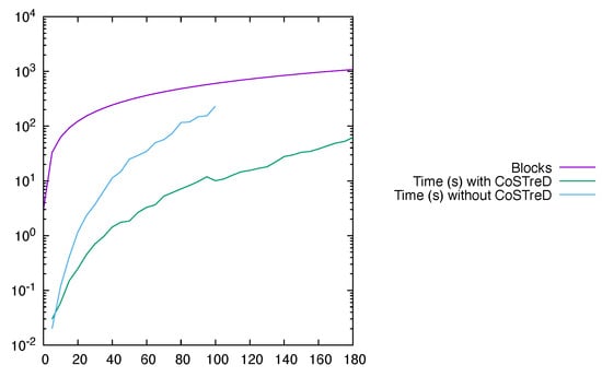
Figure 20.
Performances of the IsamDAE tool for the structural analysis of long modes of the transmission line model. The abscissa is the number N of lump elements in the transmission line. The purple curve gives the number of blocks of the Conditional Dependency Graph (CDG). The blue curve is the processor time (in seconds) with CoSTreD disabled, while the green curve gives the processor time with CoSTreD enabled.
7. Consistent Initialization of Multimode Systems
The seminal article [3] by Pantelides introduced structural analysis as a way of ensuring the consistent initialization of a DAE system. As a matter of fact, the results of the structural analysis of a DAE system yield both the set of state variables, that have to be given initial values, and the set of constraints that have to be satisfied by these values.
In the Modelica language, initial values and, more generally, initial equations, can be provided by the model designer; in Section 7.1 below, we show how this information can be used, alongside the results of structural analysis, for either ensuring that there exists a (structurally) unique initial solution, or returning diagnostics to the model designer so that they may provide adapted initial equations to their model.
We then explain, in Section 7.2, the new issues that come with the initialization of multimode DAE models, and propose a notion of initialization scenarios that help alleviate these issues. The multimode structural analysis of the resulting initialization problem is then built on the same algorithmic building bricks as already used for the analysis of long modes.
7.1. Consistent Initialization of DAE Systems
The structural analysis of a single-mode DAE system (see Section 4.3) yields orders of differentiation for the equations and orders of differentiation for the variables, such that the system
is structurally nonsingular with respect to its leading variables , ⋯, . The solution manifold is then defined by the system
which is an equation system only involving the state variables
The consistent initialization problem consists in determining an initial value for that satisfies all constraints given by ; in this context, system is regarded as an algebraic system, and is generically underdetermined.
A set of initial equations must then be specified so as to uniquely define the initial value of ; in particular, the system must then be structurally nonsingular with respect to the variables .
A possible tool for checking this property, and returning precise diagnostics to the model designer if it is actually violated, is the Dulmage–Mendelsohn decomposition introduced in Section 4.2. System is structurally nonsingular if and only if the sets and (resp., the underdetermined and overdetermined subsets of equations) returned by the DM decomposition are empty. Otherwise, these sets provide valuable information about which initial equations should be added, removed or changed in order to ensure (in a structural fashion) the existence and uniqueness of the initial state.
Note, however, that the current Modelica tools do not provide such advanced diagnostics for consistent initialization. In general, no information about the results of structural analysis is returned to the user, so even the set of state variables may not be known to them. On the contrary, we advocate that useful information given by the DM decomposition of the initialization system should be provided to the user in order to help them provide adapted initial equations in their model. In what follows, we show how the DM decomposition-based approach detailed above can be extended to handle initialization scenarios for multimode DAE systems.
7.2. Extension to Multimode Systems
In the multimode setting, the set of consistency equations is a mode-dependent set . As a direct consequence, issues related to both decidability and determinism appear when trying to extend consistent initialization to multimode DAE systems.
One such issue is that providing a single mode-independent set of initial equations is, in general, not sufficient for ensuring the uniqueness of the initial state of the system, as there may exist several modes in which the system is structurally nonsingular. In such cases, a nondeterministic choice of the initial mode among those would lead to obvious drawbacks related to reproducibility issues, but also to faithfulness to an expected initial behavior.
These problems could be avoided for models in which the mode is uniquely determined by values of state variables, but deciding whether this is the case for a given multimode model is a difficult problem, with little hope for an automatic decision procedure.
For these reasons, the approach detailed in the remainder of this section is based on the notion of initial scenarios. An initial scenario is defined by a set of initial equations, together with a non-empty set of corresponding initial modes. It is implied that initial scenarios are mutually exclusive; the relaxation of this assumption is considered by the authors as future work.
Each (possibly differentiated) equation that has to be taken into account for consistent initialization, be it an initial equation declared in the model or a consistency equation given by the results of the multimode structural analysis, is associated with a fresh Boolean variable; let be the set that collects these variables. A similar process holds for the variables, that can be either algebraic variables declared and used only in an initialization scenario, or state variables given by the results of structural analysis; set collects these variables. Edges are defined in a way similar to what is performed for the structural analysis of long modes (see Section 4.3), so that set is in one-to-one correspondence with a subset of . Last but not least, a fresh Boolean variable is associated with each initialization scenario, and set is the set of all possible valuations of these variables (This encoding was chosen for the following reason: one can expect that the number of initialization scenarios defined in a model remains very small compared to the size of the model so that this “unary encoding” will not significantly impact computational times).
The functions representing all structural information needed for the structural analysis of consistent initialization are given in Table 2; they are once again generated from parsing the original model.
Table 2.
Functions generated from parsing the model.
Two observations are made in order to highlight and explain the differences with Table 1 (Page 12), which gives the structural information needed for the structural analysis of long modes:
- The invariant involves both modes and initialization scenarios, returning if and only if is a possible initialization scenario and is a possible initial mode in this scenario;
- Edges are unweighted, as the system of equations for consistent initialization is regarded as a purely algebraic system.
Our multimode consistent initialization then consists of three phases.
- Select one matching of maximal cardinality for each scenario and each mode, that is, for each pair such that holds; this information is represented by functions for , each of which indicates for which initialization scenarios and in which modes the edge is part of the chosen matching.
- Compute the multimode Dulmage–Mendelsohn decomposition of the system for each initialization scenario and each corresponding initial mode.
- If the over- and underdetermined subsets are empty, the consistent initialization problem is well-posed; otherwise, return diagnostics to the user.
Step 1 can be performed in a way similar to that detailed in Section 4.3 for the solving of Pryce’s primal problem, where the set of modes is replaced with the set of modes and initialization scenarios, and maximal matchings are kept instead of MWPMs. More efficient implementation in IsamDAE is based on the use of the CoSTreD method introduced in Section 5.
Step 2 makes use of the multimode DM decomposition presented in Section 4.2. Set is replaced with set once again, and function is provided as a fixed constraint on the set of modes and scenarios in which the decomposition has to be performed.
Step 3 exploits the Dulmage–Mendelsohn decomposition of the system for outputting diagnostics, in a way similar to the diagnostics for the structural analysis of long modes (Section 6.1). Initial scenarios and modes of interest here are those in which the under- and/or overdetermined blocks of the decomposition are non-empty.
8. Structural Analysis of Mode Changes and Generation of Restart Conditions
So far, we addressed “long” modes, in which the dynamics are governed by a (mode-dependent) DAE, and consistent initialization. The next question is: how to determine the restart conditions for the new mode upon the occurrence of a mode change?
To convince oneself that this is a new issue, different from that of consistent initialization, one may consider again the clutch model introduced in Section 2.3. Its consistent initialization possesses two degrees of freedom when the clutch is released (the angular velocity of each shaft), and one degree of freedom when the clutch is engaged (the common angular velocity). In contrast, the physics tells us that the restart at both mode changes (engaged→released and released→engaged) is determined, i.e., possesses zero degrees of freedom. It turns out that the synthesis of consistent restart conditions at mode changes requires by itself a specific structural analysis.
As far as we know, this issue was totally open before we started working on it. Specific solutions were available for restricted physics (electrical circuits, contact mechanics, and a few more), but the issue was not considered in its generality, in a physics-agnostic setting. Our approach was first announced and sketched in [34]; Ref. [35] gives an informal presentation and identifies the agreement of our approach with a direct, more classical, approach for the so-called “semi-linear” systems; Ref. [7] develops the mathematical foundations needed for our approach, with an extensive development of the nonstandard analysis bases; Refs. [8,9] explains our approach to structural analysis and impulse analysis at mode changes, based on illustrative examples.
In this section, we propose a structural analysis for mode changes and we explain how the result of this structural analysis provides:
- A diagnosis of the mode change model, from the perspective of mode changes: they can be structurally regular, or over/under-specified;
- A first step in generating effective restart conditions to be evaluated at runtime (for a structurally regular mode change model).
8.1. Infinitesimal Time Discretization
If DAE dynamics are approximated in discrete time, then the whole model becomes discrete-time. To avoid the problem of the approximation error, our idea is to use an “infinitesimal” time step in the discrete-time approximation. This will yield an approximation up to an infinitesimal accuracy. This can be made rigorous by relying on nonstandard analysis [7,16,17], which extends the set of real numbers to a superset of hyperreals that includes infinite sets of infinitely large numbers and infinitely small numbers. For the understanding of what follows, it is enough to know the following about nonstandard analysis.
- There exist infinitesimals, defined as hyperreals that are smaller in absolute value than any real number. The arithmetic operations +, ×, etc., and usual relations, are lifted to .
- For every finite hyperreal , there is a unique standard real number such that is infinitesimal, and is called the standard part (or standardization) of x. Standardizing functions or systems of equations, however, raises difficulties.
- For an -valued (standard) signal (), denote the nonstandard internalization of x (see [17], Section I.2).
In the rest of the article, the internalization of a real function f is also denoted f, instead of . This is a sound and unambiguous abuse of notation, since for all .
We then consider the time index set :
where denotes the set of hyperintegers, consisting of all integers augmented with additional infinite numbers called nonstandard, and ∂ is an arbitrary, but fixed, infinitesimal (It is proved in [7] that the simulation code that is finally generated does not depend on the choice of this infinitesimal time step). The following features of are important:
- Any finite real time is infinitesimally close to some element of (hence, covers and can be used to index continuous-time dynamics); and
- is “discrete”: every instant has a predecessor (except for ) and a successor .
Let x be a nonstandard signal indexed by . The forward- and backward-shifted signals and are defined by:
implying that an initial value for must be provided. For a function of the tuple X of signals, we set where the forward shift applies pointwise to all the components of the tuple. For example,
Using (33), we represent, up to an infinitesimal, the derivative of a signal by its first-order explicit Euler approximation . Solutions of multi-mode DAE systems may be non-differentiable or even non-continuous at events of mode change. To give a meaning to at any instant, we define it everywhere as
8.2. The Clutch Example
The nonstandard expansion of the clutch model (System (2), page 8) is:
The multimode structural analysis of this system has already been performed, finding that equation has to be differentiated once in mode . Note that the resulting differentiated equation is replaced by the forward shifted equation ; both are equivalent from a structural point of view. The state variables are , whereas the leading variables are now , , , , in both modes and . This yields a sort of explicit Euler scheme for the model (2), which is exact up to infinitesimals within each mode. This yields a sort of explicit Euler scheme for model (2), which is exact up to infinitesimals within each mode.
- Structural analysis of mode changes
We now proceed, for this example, to the structural analysis of mode changes, and we focus on the difficult mode change , when the clutch gets engaged. At the considered instant, we have and . We unfold System (36) at the two successive (previous and current) instants by taking the actual values for the guard at those instants into account:
We regard System (37) as an algebraic system of equations with dependent variables for , i.e., the leading variables of System (36) at the previous and current instants. System (37) is structurally singular, as it includes the following subsystem (Over- and underdetermined subsystems are structurally found by computing the Dulmage–Mendelsohn decomposition of the system, see Section 4.2) which has five equations and only four dependent variables :
This conflict is due to the superposition of predictions of current velocities by the previous mode, and consistency constraints set by the new mode. Should we decide that this makes the model incorrect and reject it? Not quite: this is an artifact of discretization. So, we decide to resolve this conflict, while applying the following principle:
Principle 1
(causality). What was performed at the previous instant cannot be undone at the current instant.
Applying Principle 1 leads to removing, from subsystem (38), the conflicting equation . This yields the following nonstandard code for the restart at mode change :
The consistency equation has been removed from System (39), thus modifying the original model. However, this removal occurs only at mode change events , thus only for a single nonstandard instant. What we have achieved amounts to delaying by one nonstandard instant the satisfaction of some of the constraints in force in the new mode . Since our time step ∂ is infinitesimal, this takes zero standard time, and, thus, causes no harm.
- Generating effective code for restart
We wish to use System (39) by identifying current values for the states with the left-limits , i.e., the values of the velocities just before the mode change. From these values, we would then compute the restart values for the velocities , together with the torques .
Unfortunately, hyperreals are unknown to computers, hence, System (39) cannot be used as such, but needs to be standardized, by “washing out” ∂. Since the time step ∂ is infinitesimal, it is tempting to get rid of it in (39) by simply setting . Unfortunately, doing this leaves us with system
which is structurally singular. This exemplifies the difficulty in standardizing systems of nonstandard algebraic equations. Indeed, the following key result is proved in [7]:
Theorem 3.
For a (standard) function, consider the nonstandard system of equations where X is a n-vector of variables. If system is structurally nonsingular, then setting in system yields the correct standardization of it, meaning that the solution of standardizes as the solution of .
Theorem 3 states in particular that brute force setting in system (39) is not the correct way of standardizing this system when this yields a structurally singular system.
The cause of structural singularity of System (40) is the existence of impulsive variables. To discover impulsive variables, we perform an impulse analysis. Before engaging the clutch, we must assume , generically. As a result of the engagement, holds, thus causing a discontinuity in the velocities. Hence, cannot be finite because, if it was, then, would be of order ∂, meaning that the function is continuous (see (32)), a contradiction. Hence, the hyperreal is necessarily infinite. However, we assumed continuous functions and finite state . Thus, one of the torques must be infinite at mode change, and because of equation , both torques are in fact infinite, i.e., are impulsive.
We can get rid of this problem by eliminating impulsive variables. To make this feasible, we now assume that the ’s are linear in the torques, i.e., each has the form
where and are the inverse moments of inertia of the rotating masses and and are damping factors divided by the corresponding moments of inertia. This yields the following system of equations, to be solved for at the instant when switches from to :
We now eliminate the impulsive variables from System (41), namely, the two torques. Using yields . Premultiplying the system of equations
by the row matrix yields
Using in addition and setting yields
It is now legitimate to standardize the right-hand side by setting in it. This yields, by identifying and :
where we recall that is the standard part of , see the beginning of Section 8.1. Equation (42) provides us with the reset values for the positions in the engaged mode, which is enough to restart the simulation in this mode.
Figure 21 shows a simulation of the Clutch where the resets are computed following this approach. As expected, the reset value sits between the two values of and when (at s), and the transition is continuous at the second reset (at s). An alternative approach for the computation of the reset values, which does not require the elimination of impulsive variables, is developed in [7], see also Section 9.
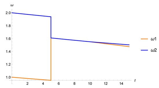
Figure 21.
Simulation of the Clutch model with resets. Mode change occurs at s and mode change occurs at s.
The clutch example exhibited mode changes with impulsive behaviors. One more difficulty can arise, which is not present in the clutch, namely: the existence of transient modes, which are left immediately after being reached.
Such a situation occurs in the Cup-and-Ball example we develop in this section, see Figure 22. This example is a multimode extension of the popular example of the pendulum in Cartesian coordinates [3]. A ball, modeled by a point mass, is attached to one end of a rope, while the other end of the rope is fixed, to the origin of the plane in the model. The ball is subject to the unilateral constraint set by the rope, but moves freely while the distance between the ball and the origin is less than its length. The system is assumed closed. The model for a 2D-version of this example is:
where the dependent variables are the position of the ball in Cartesian coordinates and the rope tension .

Figure 22.
The Cup-and-Ball game.
8.3. The Cup-and-Ball Example
The subsystem expresses that the tension is nonnegative, the distance of the ball from the origin is less than or equal to L, and one cannot have a nonzero tension and a distance less than L at the same time. Constraints and are unilateral, which is not supported by Modelica and related languages. Therefore, using the technique presented in [36], we redefine the graph of this complementarity condition as a parametric curve, represented by the following three equations:
Similarly to the Clutch model, impulsive behavior is expected in the torques. However, an other possible difficulty is present: subsystem of (43) leaves the impact law at mode change insufficiently specified; it could be elastic, or inelastic. What are the consequences of this missing specification?
Two issues have to be addressed by our structural analysis: the expected impulsive behavior of the accelerations at mode changes, and the insufficient specification of the nature (elastic or inelastic) of the impact.
Equation (46) means that the derivatives are interpreted using the explicit first-order Euler scheme with an infinitesimal time step∂. Note that (46) implies
After performing the substitutions given by (46), we observe that the subsystem collecting equations – is a logico-numerical fixpoint equation, with dependent variables . A possible solution would consist in performing a relaxation, by iteratively updating the numerical variables based on the previous value for the guards, and then re-evaluating the guard based on the updated values of the numerical variables, hoping for a fixpoint to occur. Such a fixpoint equation, however, can have zero, one, several, or infinitely many solutions. No characterization exists that could serve as a basis for a (graph-based) structural analysis. We thus decide to refuse to solve such mixed logico-numerical systems.
As a consequence, we are unable to evaluate guard , so the mode that the system is in cannot be determined: model (45) is rejected.
To break the fixpoint equation defining , we choose to systematically introduce infinitesimal delays to guards. For the Cup-and-Ball, the predicate then defines the value of the guard at the next nonstandard instant (The condition triggering the mode change is based on the positions, which remain continuous at mode changes, even though the velocities are discontinuous. As a result, the shifting of this guard by an infinitesimal time step only yields an infinitesimal change in the values of state variables, which will be erased by the standardization process so that the numerical solution is not impacted by this change in the model). This yields the corrected model (48), where the modification is highlighted in red.
This model is understood in the nonstandard setting, meaning that the derivatives are expanded using (46). The leading variables in all modes are .
- The Cup-and-Ball in Modelica
Figure 23 details the Modelica model of the Cup-and-Ball game. It is a faithful translation of the two-mode DAE (43) using rewriting (44). The point mass, modeling the ball, initially stands at the origin of the plane with zero velocity; the Boolean guard , named gamma in the model, is thus set to false.
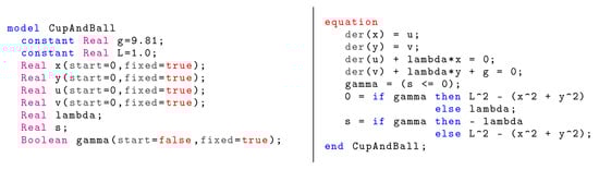
Figure 23.
Modelica code for the Cup-and-Ball.
As is the case for the clutch model presented above, this model is deemed structurally nonsingular by both OpenModelica 1.17.0 and Dymola 2021, but the simulation fails at the instant of mode change. Figure 24 depicts the resulting trajectory of variables y and gamma; it ends when gamma switches from false to true, as the tool is unable to correctly reinitialize the model after the mode change. Replacing condition s <= 0 with last(s) <= 0 in order to break the fixpoint equation defining variable gamma (see modified model (48)) leads to the same simulation results, but with a division by zero error similar to that shown in Figure 10 occurring at the moment of mode change.
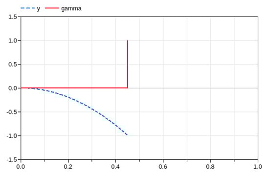
Figure 24.
Trajectory of the Cup-and-Ball Modelica model: it stops around s, when the rope becomes straight.
- Structural analysis of mode changes
Due to equation , the mode (where the rope is straight) requires index reduction. We thus augment model (48) with the two latent equations shown in red:
Note that, as in System (36), the two latent equations and were obtained by shifting forward, which is equivalent to differentiating it for the structural analysis. To perform structural analysis at the considered mode change, we unfold model (49) at the successive instants
where t denotes the current instant. In the following, equation at the instant (respectively, ) will be denoted by (resp., ).
In this unfolding, the two equations and are in conflict with selected equations from the previous two instants, shown in blue in the following subsystem, whose dependent variables are the leading variables at instants and , namely :
We resolve this conflict by applying causality Principle 1, which leads to erasing, in model (49), equations and at the instant of mode change . This yields:
System (50) uniquely determines all the leading variables from the state variables and . In turn, equations and , which were erased from this model, are not satisfied. At the next instant, i.e., when , the same argument is used. We thus erase, in model (49), the only equation at the next instant. This yields:
Note that is a consistency equation that is satisfied by the state variables . In turn, equation , which was erased from this model, is not satisfied. At subsequent instants, equation erasure is no longer needed.
This completes the nonstandard structural analysis of the mode change , i.e., when the rope gets straight.
- Generating effective code for restart
Code generation for restarts consists in standardizing nonstandard systems (50) and (51), in a way similar to Section 8.2. We focus on the standardization of the mode change , i.e., when the rope gets straight. Our task is to standardize systems (50) and (51), by targeting discrete-time dynamics, for the two successive instants composing the restart phase. This will provide us with restart values for positions and velocities.
Due to the expansion of derivatives in equations , tensions and are both impulsive, hence so are s and by . We eliminate the impulsive variables by ignoring , combining and to eliminate , and and to eliminate . This yields:
In System (52), we expand second derivatives using (46), whereas in System (53) we expand them using (47). Consequently, (52) has dependent variables , whereas (53) has dependent variables . We are now ready to standardize the two systems.
Setting in this system yields a structurally regular system. Thus, the correct standardization of System (54) is the following system:
In the resulting system, we interpret x and as the left-limit of state variable x in the previous mode, and as the restart value for the new mode. This yields
which determines the restart values for positions. The constraint that the rope is straight is satisfied. Furthermore, as also holds (the rope is straight at the mode change), is the unique solution of (55): positions are continuous.
We will use System (53) to define restart velocities. We discard the second equation of (53) since it is a consistency equation involving no dependent variable. We then expand second derivatives using (47):
By expanding , the right-hand side of the last equation rewrites
Setting in (58) yields
where we recall that the dependent variables are —other variables are state variables whose values were set at previous time steps. System (59) is structurally regular, hence, by Theorem 3, it is the correct standardization of System (56).
To obtain effective code for restart, we perform, in (59), the following substitutions, where superscripts and denote left- and right-limits, and continuity of positions is used:
and similarly for y. This finally yields
System (61) determines and , which are the velocities for restart. The second equation guarantees that the velocity will be tangent to the constraint. With (55) and (61), we determine the restart conditions for positions and velocities. Invariants from physics are satisfied.
Our reasoning so far produces a behavior in which the two modes (free motion and straight rope) gently alternate; the system always stays in one mode for some positive period of time before switching to the other mode. This indeed amounts to assuming that the impact is totally inelastic at mode change, an assumption that was not explicit at all in (48). So, what happened?
In fact, the straight rope mode was implicitly assumed to last for at least three nonstandard successive instants, since we allowed ourselves to shift twice while the system was in straight rope mode. To address elastic impact, we thus need to revise our reasoning, by not allowing ourselves to shift equations within a transient mode, having zero duration.
8.4. Handling Transient Modes
We will illustrate this on the Cup-and-Ball example, by discussing the case of elastic impact, represented by the cascade of mode changes . This cascade captures that the straight rope mode is transient (it is left immediately after being reached).
Consider again model (48). We regard the instant of the cascade when occurs as the current instant. We cannot add latent equations by simply shifting , since these shifted versions are not active in the mode . Set
Systems and are obtained by shifting once the equations constituting and ; systems and are defined similarly for all . Consider the differentiation array originally proposed by [37], except that we take into account the trajectory for guard . Using shifting instead of differentiation yields the following difference array:
The dependent variables of System are , whereas , must be eliminated. We look for the smallest n such that is structurally nonsingular in this sense. Unfortunately, although shifting twice in System (48) produces one more equation involving the leading variables , this equation also involves the new variable , which keeps the augmented system underdetermined; shifting other equations fails as well. Therefore, the structural analysis rejects this model as being underdetermined at transient mode .
The user is then asked to provide one more equation. For example, they could specify an impact law for the velocity by providing the equation , where is a fixed damping coefficient. This is reinterpreted in the nonstandard domain as , yielding the following refined system for use at mode within the cascade :
The modified difference array is now structurally nonsingular. The so modified model is accepted and two-step restart code for the mode change is generated as before.
- Declaring transient modes
Through the Cup-and-Ball example, we demonstrated the need for the following user-given information: is the current mode long or transient? Long/Transient is an information regarding modes, that cannot be found by an automatic inspection of the model. It must be inferred from understanding the system physics and must be manually specified. The natural way of performing this is to provide a different syntax for specifying long modes, on the one hand, and events corresponding to transient modes on the other hand (mode changes separating two successive long modes need not be specified).
The ‘if’ and ‘when’ statements of the Modelica language are fit candidates for this purpose. We devote the ‘if’ statement to long-lasting modes specified by a predicate, while the ‘when’ statement, pointing to the event when a predicate switches from to , could be further restricted to be a zero-crossing condition, by which a -valued expression crosses zero from below [38]. Using this feature, the Cup-and-Ball example with elastic impact is specified as follows:
8.5. Multimode Structural Analysis in General
We restrict ourselves to the following class of multimode DAE systems:
- We consider only systems possessing long modes (having DAE-based dynamics for a positive duration) alternating with finite cascades of transient modes (having a zero duration, such as the straight rope mode in the Cup-and-Ball model with elastic impact).
- We assume that the information regarding the type of a mode (long vs. transient) is known by the compiler—the two different Modelica primitives if and when should be used to declare long and transient modes, respectively.
- In addition, we require that the current mode is defined by the left-limits of some predicates, see the reasoning leading to the corrected model (48) for the Cup-and-Ball.
For such models, the structural analysis proceeds as follows. Having multiple modes does not change anything in the way the dynamics should be handled within each long mode: just perform the structural analysis of the DAE attached to that mode.
Hence, from theoretical standpoint, we just need to focus on the handling of finite cascades of transient modes separating two successive long modes. Which cascades are actually visited can only be determined at run time, which requires simulation code—unfortunately, this is precisely what we are working at in our analysis. To break this circular reasoning, we need to explore hypothesized cascades of transient modes. A brute force approach would consist of (1) exploring all the possible modes (defined by the assignment of a value to all Boolean variables), and (2) exploring all combinations of successive modes to define the above-hypothesized cascades. This clearly leads to a risk of combinatorial explosion. It is therefore essential to bound this exploration by using prior information derived from the program syntax. How to perform this at compile time is discussed in ([7], Section 6.4.3).
For the structural analysis of such a cascade, we use a first-order explicit Euler expansion for derivatives, with infinitesimal time step ∂. Then, we partition the ∂-discretized timeline as follows, where denotes the first instant when the previous long mode is left:
In (63), the long mode just before the cascade is shown first, we call it the entry mode. It is followed by the cascade of transient modes, and ends with the long mode following the cascade, which we call the exit mode. We split the latter into a restart phase, taking instants, and a steady phase, where normal DAE dynamics operate. The DAE dynamics of the exit long mode is index reduced: latent equations found by the -method are added to the DAE model, within the restart phase of the exit mode.
In (63), Integer is the maximum differentiation degree of the DAE acting in the entry mode. Integer is the maximum forward shifting degree occurring in the (discrete-time) dynamics of the cascade of transient modes, in the nonstandard semantics. These choices for k and l ensure that we cover the entire time interval where entry and exit dynamics may interfere with the dynamics of the cascade.
At this point, we consider the time-interval and we collect all the (discrete time, nonstandard) equations attached to this interval. With reference to Campbell-Gear notion of differentiation array [37], we call the resulting system of equations the difference array attached to the cascade, and we denote it by . Its free variables are all the variables set by the entry mode (before the mode change), and its dependent variables are all the leading variables for the instants t ranging over the interval . The structural analysis of array proceeds as follows:
- Apply Dulmage–Mendelsohn decomposition with respect to the dependent variables of the array, which partitions the array into its over-determined, regular, and under-determined parts.
- Remove conflicts by considering the subarray , and apply again Dulmage–Mendelsohn decomposition with respect to the same set of dependent variables—we know that the over-determined part of this decomposition will be empty. Then,
- If is non-empty, we return to the user the set of undetermined variables and warn that the model is insufficiently specified.
- Alternatively, if is empty, the structural analysis of the array succeeds and we can move to generating restart conditions for the long exit mode, using .
The above procedure is formalized in Algorithm 2.
| Algorithm 2 Structural analysis of mode changes |
|
- Important remark: The algorithm presented in Definition 2 involves two successive calls to the Dulmage–Mendelsohn decomposition, without any explicit reference to a particular mode. Note, however, that the difference array itself is attached to a cascade of (transient) modes, i.e., it depends on a mode trajectory. Therefore, an efficient implementation of this algorithm must use our dual representation of mode-dependent dynamics, presented in Section 4.1, and extensively used in the presentation of algorithmic building blocks in Section 4. The implementation of the two successive calls to Dulmage–Mendelsohn decomposition in the algorithm of Definition 2 must rely on the multimode extension of this method, as presented in Section 4.2. The software implementation of the algorithm presented in Definition 2 is in progress.
The number of hypothesized cascades can be very large (worse than the number of modes), hence, applying the above-described algorithms as such would be very inefficient. Work is ongoing to carry over the implicit multimode extension of the -method (Section 4.3) to the implicit handling of cascades; the key algorithmic component of this work if the multimode Dulmage–Mendelsohn decomposition presented in Section 4.2, and implemented in the IsamDAE tool.
The approach developed in this Section is a systematic way to define the solution of a multimode DAE system. The use of implicit “dual” representations, such as the ones used in the IsamDAE tool, will allow applying this approach to large-scale and/or multi-physics models.
However, this approach still presents several other difficulties regarding its possible mechanization in a tool. We list below the main three developments that are required for its automatization and hint at how we are addressing them:
- Identification of impulsive variables. We present in Section 9 a calculus for this, which is ready for automatization (this is under development in our IsamDAE tool).
- Elimination of impulsive variables. This is easy if impulsive variables enter linearly in the model—this was the case for the Clutch and Cup-and-Ball examples. It is highly costly but still doable if impulsive variables enter polynomially in the model, but cannot be performed practically in all other cases. As a result, the elimination of such variables only seems adapted in practice to a subclass of multimode models in which these variables occur in a linear fashion. Alternative approaches for the handling of impulsive variables are proposed in Section 9.
- Clever choice of how to map nonstandard variables to restart conditions. This was straightforward for the Clutch, but definitely not for the Cup-and-Ball (Section 8.3), where expansion (46) for the derivatives was used for resetting positions, whereas expansion (47) was used for resetting velocities. Works are in progress for automating this choice.
9. Impulse Analysis
As discussed above, a specific focus is required on the detection of impulsive behaviors. In this section, we propose a calculus by which impulsive variables can be identified at compile time, with a quantitative characterization of their magnitude order in terms of the discretization time step. The approach is developed on the Cup-and-Ball example, then generalized. Possible methods that can be used for computing actual restart conditions, from the knowledge of impulsive variables and their respective magnitude orders, are also illustrated in the same example.
Our impulse analysis not only identifies impulsive variables but also quantifies their order of magnitude, thanks to the following notion of impulse order:
Definition 5
(Impulse order and analysis). Consider a nonstandard system of equations E defining the values for restart.
- 1.
- A dependent variable x has impulse order in Eif and only if the solution of system E is such that is provably a finite non-zero (standard) real number. The impulse order of x, when exists, is denoted .
- 2.
- x is impulsive if . By convention .
- 3.
- The impulse analysis of a system of equations S is the system of constraints satisfied by the impulse orders of the dependent variables of S.
Remark that impulse orders may be rational or irrational numbers. The latter is often the case when nonlinear equations are considered. For instance, equation , where , entails the fractional impulse order . Equation then yields the irrational impulse order .
Impulse analysis relies on the following generic assumption, which expresses that DAE within long modes must be reinitialized with finite values for the state variables:
Assumption 1.
State variables are not impulsive; that is, for any state variable v, one has .
As an example, if, in the new mode, a variable x is differentiated up to order n, then its -th derivative is a state variable and thus subject to Assumption 1. Consequently, its k-th order derivatives for are continuous at the considered mode change.
9.1. The Cup-and-Ball Example
Here we focus on identifying possible impulsive behaviors at mode change . This is achieved by analyzing nonstandard systems (50) and (51) defining the values for restart. The intent is that the former will set the restart positions, whereas the latter will set the restart velocities. We successively analyze Systems (50) and (51).
For System (50), the state variables are . By Assumption 1, we obtain the following prior information, which expresses that velocities are not impulsive:
Conditions (64) imply that positions should be continuous. While performing our impulse analysis, we include Equation (47) relating second derivatives and first derivatives.
By (64), Equation (65) implies . Exploiting all equations of System (50) yields the following information
whereas other dependent variables have impulse order zero. System (51) is handled similarly, with the same conclusion. In Section 9.2, we mechanize the impulse analysis for an arbitrary restart system. In Section 9.3, we then explain how this impulse analysis can be exploited for generating effective code for restart.
9.2. General Impulse Analysis
Here, we explain how the reasoning used for the Cup-and-Ball example can be mechanized as a compilation stage following multimode structural analysis.
- Problem setting
Restart systems of equations, as resulting from the structural analysis at mode changes, are nonstandard systems of equations of the following generic form:
where V collects the algebraic variables, X collects the state variables, and is the nonstandard semantics of . , seen as a vector function in its arguments, is by itself standard since the equations of system are obtained by shifting or differentiating equations specified by the user. The reason for (67) being nonstandard is indeed twofold:
- Since is involved, the infinitesimal ∂ occurs in time; and
- Since is involved, the infinitesimal ∂ occurs both in time and space, due to the expansion .
The occurrence of ∂ in time is not an issue: shifted state variables will correspond to restart values for states, whereas non-shifted ones correspond to values prior to the change. In contrast, the occurrence of ∂ in space is the root cause of possible impulsive behaviors. Identifying them is the subject of impulse analysis.
- The rules of impulse analysis
We now develop the impulse analysis introduced in Definition 5. This analysis is useful as a postprocessing of structural analysis, prior to generating effective code for restarts. Note that Assumption 1 is still enforced in what follows.
Figure 25 and Figure 26 display the rules defining the translation of a system of equations of the form (67) into its impulse analysis, for the restricted class where only rational expressions are involved.
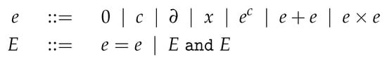
Figure 25.
Syntax: E is a system of one or several equations e = e. An expression e is 0, a nonzero
(standard) real constant c, the infinitesimal ∂, a variable x, the monomial ec, a sum, or a product.
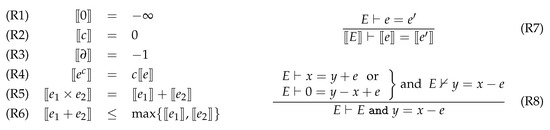
Figure 26.
Rules: The left column displays the impulse order of the primitive expressions. Rule (R7) indicates that is an equation of the impulse analysis if is an equation of E; rule (R8) indicates that, if E involves the equation but not the equation , then we augment E with the latter, i.e., we saturate E with the rule .
Figure 25 describes the syntax of a mini-language specifying such systems of equations. The left column of Figure 26 gives the rules for mapping expressions to their corresponding impulse orders.
The reason for the inequality in (R6) is that in the sum , the dominant terms in the expansion of as a series over ∂ may cancel each other. For an example of this, see equation in System (51): rewriting this equation as , we see a case of strict inequality for (R6) since gravity g has order zero, whereas it is equal to the difference between two terms of order one. We will use Rule (R6) in the following way, thereby reinforcing it. Consider, for example
We can rewrite equation e in the following equivalent ways: , or . To each of them we apply the max rule. This yields the following system of constraints called the impulse analysis of equation e:
Note that the constraint is vacuously satisfied since . Then, among the three nontrivial inequalities of (68), at least two of them must be saturated. We will use impulse analysis (68) for handling sums of terms. This reinforcement of the max rule is formalized by Rule (R8) of Figure 26, which mechanizes the association, to any equation, of its different rewritings.
9.3. Computing Restart Conditions
Code generation for restarts consists in standardizing nonstandard systems such as Systems (50) and (51). See Section 8.1 for the meaning of “standardization”. Standardizing systems of equations requires more care than standardizing numbers, due to impulsive behaviors and singularity issues that result, see also Theorem 3. We can exploit the impulse analysis using three different methods. The first method is mostly described for didactic purposes, as it requires the symbolic elimination of variables, which can be very costly or even impossible in nonlinear systems. In practice, the second and third methods shall be used.
- Eliminating impulsive variables
When this is practical, the simplest method from a conceptual point of view is to eliminate impulsive variables from the restart system, as they are of no use for restarting the new mode. This is a satisfactory solution when the elimination of impulsive variables is practical. In our example, they entered linearly in the restart system, so that elimination was straightforward. When this is not the case, elimination becomes costly or even impossible. Moreover, generalizing and mechanizing this elimination process appears to be a very difficult task. We thus need to look for alternatives for computing the velocities for restart.
- Rescaling impulsive variables
Focus again on System (51). Impulse analysis told us that both have impulse order . We thus rescale them accordingly:
In System (70), is a consistency equation satisfied as a result of performing (50) at the previous instant. We can also discard equation , which only serves to determine the auxiliary variable s. Thus, we are left with the sub-system collecting equations . We can again expand the right-hand side of by using (57). In the resulting system, by Theorem 3, we can safely set since it yields the following structurally regular system:
System (71) determines , and the rescaled impulsive tension , as functions of state variables , which were identified with the left-limits of velocities and positions at previous mode. Note that eliminating the rescaled tension from System (71) yields System (55).
Rescaling impulsive variables is simpler than eliminating them. This method is also promising in terms of designing and implementing algorithms for its mechanization, as the computation of the impulse orders amounts to finding a minimal solution to a system of linear unilateral constraints. Unfortunately, it does not work in full generality since impulse orders can be infinite, as the following example shows:
where y is known to have impulse order zero. Indeed, the impulse order of is n. Since the exponential expands as a power series of infinite support, we deduce that the impulse order of is the maximum of all impulse orders of , hence it is infinite. Thus, the impulsive variable x cannot be rescaled. The last method addresses such cases, at the price of a possibly poor numerical conditioning.
- Bruteforce solving of the restart system
When none of the above methods apply, it is still possible to solve the system returned by the structural analysis of a mode change with (a small positive time step) for its original variables. In the Cup-and-Ball example, System (51) would be solved, with , for the original variables and s. Then, it is proved in [7], see also [8], that solving these systems for their dependent variables and then discarding the values found for the impulsive variables yields a converging approximation for the states and velocities at restart. The first numerical experiments on toy examples showed no issue as long as the time step was kept reasonably high. Of course, without rescaling, the numerical conditioning is less favorable, so rescaling is recommended when impulse orders are finite. Work is in progress for the implementation of this method, coupled with the rescaling of impulsive variables when they have finite order.
10. A Model Transformation for Multimode Modelica Models
In this section, we demonstrate how multimode structural analysis can be used for transforming a multimode Modelica model into its RIMIS (Reduced Index Mode-Independent Structure) form, which is guaranteed to yield correct execution on state-of-the-art Modelica tools. This method is illustrated in the Water Tank model for which current Modelica tools fail to execute. Recall that the root cause of this difficulty is that structural analysis methods implemented in these tools fail to yield the correct execution code for this model. In the present section, we demonstrate the generation of a target Modelica model under RIMIS form, resulting in a correct simulation of the model. Our approach is then formalized for its broad application to problematic multimode models.
10.1. A Reduced Index Mode-Independent Structure (RIMIS) Form
Using multimode structural analysis to transform a multimode Modelica model into a reduced-index model, that simulates correctly with state-of-the-art Modelica tools, is made difficult by the fact that the Modelica language does not permit to enable or disable an equation depending on the mode. Based on this limitation, the basic principle of our model transformation is to evaluate all equation blocks of the CDG in a mode-independent fashion, irrespectively of the mode in which the system is. Of course, this leads to useless computations during simulation. However, this turns out to be a systematic way to ensure a correct simulation of multimode Modelica models.
The model transformation is detailed below, in informal terms, then illustrated on a simple example. A mathematical definition of the transformation is detailed in Section 10.4. Remark that models with either initial equations, or when, or reinit statements, are not covered in this paper. Further, note that models with non-scalar variables or class instances of any kind are not considered here. It is assumed that the models have been flattened according to the procedure described in Chapter 5 of the Modelica Language Specification [18]. It is also assumed that all mode variables are of type Boolean.
The method decomposes in the following seven steps:
- Conditional Dependency Graph: The CDG of the source model is computed by the multimode structural analysis method. This graph defines a block-triangular decomposition of the reduced-index system, for each mode of the system. It will be used throughout the transformation.
- Source Model Variable Declarations: Variable declarations from the source model are copied unchanged, with the exception of real variables, whose initialization parts are removed.
- Replicate and Dummy Derivative Variables: For each block of the CDG, replicates of written variables (unknowns) are declared. Whenever an unknown appears differentiated, a dummy derivative variable [2] is declared. Initialization statements for state variables are copied from the source model. As an optional optimization, non-leading replicate variables can be shared among a disjunction of modes, in order to decrease the number of variables in the resulting model.
- Mode Equations: Equations defining mode variables are copied unchanged. For the sake of simplicity, these equations are assumed to be of the form b = (expr > = 0), where is a real expression.
- Replicate and Dummy Equations: Equations are replaced with replicates, according to the following principle:For each block in the CDG, equations appearing in this block are replicated, substituting (i) every written variable (unknown of the block) by the replicate declared in step 3, and (ii) every read variable (parameter of the block) by the corresponding replicate, if it is a leading variable. Both mode variables and read state variables are left unchanged.As a result, the single-mode structural analysis of the resulting equation system yields a block-triangular decomposition that contains all the blocks of the CDG obtained by the multimode structural analysis of the original model.For each equation in the fresh model, the propositional formula conditioning the block in which this equation appears can be taken into account: a partial evaluation of the equation is performed [39]. This has the effect of simplifying the equation, by eliminating some of the conditionals (if … then … else … operators).Note that the resulting equations may still be multimode: in general, not all conditionals can be eliminated by partial evaluation. However, the fact that the structure of the resulting equations is independent of the mode is still guaranteed: the multimode structural analysis ensures that each equation block has the same structure (in particular, the same read and written variables) in all the modes in which it is defined, even if one or several of its equations contain conditional statements.First-order differential equations are also added in accordance with the dummy derivatives method.
- Multiplexing Equations: In order to retrieve the values of the source model variables from the replicates in the fresh model, multiplexing equations have to be added. These are multimode equations, containing conditional operators, but these equations contain no dynamics: each multiplexing equation focuses on a source model variable that corresponds to several replicates in the transformed model, specifying which of the latter currently holds the value of the former.
- Reinitializations: Reinitialization statements finally have to be inserted, in order to reset replicate variables that are state variables to a correct value upon the occurrence of a mode switching. Therefore, these statements are triggered by mode changes.
10.2. Transformation of a Simple Model
We illustrate the method on the simplistic, yet relevant, Two Equations model (Figure 1, page 4). Recall that this model has one real equation, one Boolean equation and, that its CDG (Figure 2a) resulting from the multimode structural analysis distinguishes between two cases:
- when p is true, x is a leading variable, meaning that it is the unknown that needs to be solved;
- when p is false, the leading variable is x′, the first-order time derivative of x, while x itself is a state variable.
Recall that the approximate structural analysis of state-of-the-art Modelica tools determines that the leading variable is x′ in all modes; however, the real equation is singular in x′ when p is true. Unsurprisingly, an exception is raised during simulation, as shown in Figure 2a.
Let us apply the transformation one step after the other:
- The CDG graph of the source model is shown in Figure 2a.
- Declarations of variables x and p are copied.
Real x;
Boolean p(start=false,fixed=true);Remark that the declaration of x has been stripped of its initialization part. - Replicate variables are created according to the two blocks of the CDG. Two leading replicate variables x_2 (holding the value of x if p holds) and x_p_3 (holding the value of x′ if not p holds), and one state replicate variable x_3 that is meaningful only if not p holds, are declared.
Real x_2;
Real x_p_3;
Real x_3(start=0,fixed=true);Note that the initialization of variable x in the source model is copied here, to initialize the replicate state variable x_3. - One mode equation is copied from the source model.
p = (x >= 1); - Replicate equations are generated from the CDG, which has two blocks of one equation each.From the block p : e → x, one replicate equation is generated by replacing variable x with its replicate x_2, then performing the partial evaluation [39] under the assumption that the Boolean condition p holds.
// Block e_2 -> x_2
/* e2 : */ 1 = x_2;From the second block not p: e → x′, one replicate equation is generated in a similar way.// Block e_3 -> x_p_3
/* e3 : */ 1 = x_p_3;A differential equation is also generated, linking replicate variable x_3 with its dummy derivative x_p_3.der(x_3) = x_p_3; - One multiplexing equation is generated, to be solved for variable x.
x = if p then x_2 else x_3; - Finally, the only case in which a state variable has to be reinitialized is when entering the mode not p. The value of replicate variable x_3 is then set to be the left limit of x.
when not p then
reinit(x_3,pre(x));
end when;
The complete RIMIS form of the Two Equations model is given in Figure 27. The result of the successful simulation of this model is shown in Figure 28. Remark that the mode switching from p = false to p = true is correct, and that the reinitialization statement is never evaluated, as p remains true forever after time t = 1.
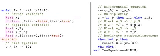
Figure 27.
Two Equations model in RIMIS form.
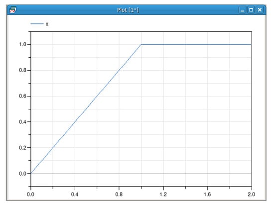
Figure 28.
Simulation of the Two Equations model in RIMIS form with Dymola 2021.
10.3. Successful Simulations of the Water Tank System in RIMIS Form
The RIMIS transformation is illustrated on the Water Tank model (Figure 4); the resulting model is shown in Figure 29. Simulation results obtained with Dymola 2021 are shown in Figure 30. It can be seen that the simulation is successful, with a correct behavior of the Water Tank system, while the simulation of the original model failed (Figure 5). A correct simulation has also been obtained with OpenModelica 1.17.0 [19], under the provision that the Newton solver is used instead of the KINSOL nonlinear solver.
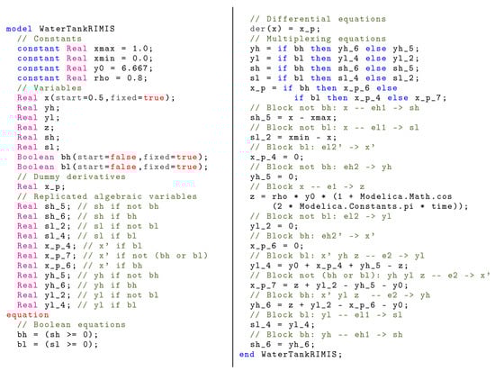
Figure 29.
The Water Tank system in RIMIS form.
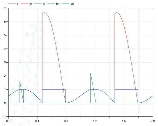
Figure 30.
Simulation of the Water Tank system in RIMIS form with Dymola 2021.
10.4. Formalizing the RIMIS Form Transformation
The mathematical definition of the RIMIS form transformation relies on the partial evaluation of equations. Once variable renaming is also properly defined, the seven-step transformation mentioned in Section 10.1 is formalized. Finally, an optimization aiming at reducing the transformed model is presented.
- Partial evaluation of expressions and equations
Partial evaluation is an umbrella name for a set of program transformation techniques that aim at specializing a program by taking into account prior knowledge on its input data, possibly improving its performances [39,40].
In the context of the Modelica language, consider a Boolean expression q, and a real expression e. The partial evaluation of expression e, assuming q, is an expression , such that q implies and , where is the set of free variables appearing in an expression.
To define the partial evaluation operator , and for the sake of clarity, we only consider the subset of the Modelica expression language defined by the following grammar, where p is a Modelica Boolean expression:
Given a Boolean expression q and a real expression e, the partial evaluation of e, assuming q, is defined by induction on the structure of e:
where
In the above definition, condition r is not unique: whenever possible, it should be chosen such that it is more concise than p.
The extension of the partial evaluation operator to equations is straightforward:
- Variable renaming
Before moving to the formal definition of the RIMIS transformation, variable renaming must be defined, in order to declare replicate variables and transform equations into their replicates.
Given a Boolean expression p, an identifier v, and a differentiation order , the replicate of the n-th order derivative of v, under condition p, is the identifier . The replication operator is assumed to satisfy the following axioms:
Checking the equivalence of two Boolean expressions is, in general, a difficult problem. In this section, Boolean expressions that appear in conditional statements are restricted to propositional formulas only. Mode equations are restricted to the form , where is an affine expression. Under these assumptions, equivalence checking can be performed with BddApron, a logico-numerical abstract domain library [41] combining BDDs (Boolean Decision Diagrams) [24] and polyhedra [42]. Such a use of BddApron is considered, among other program analyses, in Chapter 7 of [43].
- Formal definition of the RIMIS form transformation
Consider a Modelica model M that can be decomposed in the following parts:
where:
- MD is the set of mode (Boolean) variable declarations and initializations;
- RD is the set of real variable declarations, stripped of their initializations;
- RI is the set of real variable initializations;
- ME is the set of mode variable equations;
- RE is the set of real equations.
Remark that models with when and reinit statements are not covered by the RIMIS form transformation, as this would require a multimode structural analysis of mode changes [7], that is not yet implemented in the IsamDAE software [6].
Model M is assumed to be structurally nonsingular in all modes. Its CDG computed by the multimode structural analysis [6] consists of a set of blocks of equations and a set of directed edges between blocks; let Blocks and Edges denote the corresponding sets. A block consists of four parts:
- , a Boolean expression;
- , a set of equations, possibly differentiated;
- , a set of read variables (parameters of the block of equations);
- , a set of written variables (unknowns of the block of equations).
Elements of are pairs of the form , where e is an expression and is a differentiation order. Elements of and are pairs of the form , where u is an identifier and is a differentiation order. An edge consists of three parts:
- , a Boolean expression;
- , two blocks.
The meaning of an edge g is that whenever holds, block has to be solved before block . By construction, implies both and .
In addition, the multimode structural analysis computes several functions and predicates on (differentiated) variables :
- decides whether variable u is a leading variable in some mode satisfying the Boolean formula p;
- decides whether u is an algebraic variable in some mode satisfying p;
- decides whether u is a state variable in some mode satisfying p.
For the sake of clarity, the following notations are introduced: is the set of leading variables appearing in block b; is the set of blocks that define variable v in some mode satisfying the Boolean formula p, either because v itself is written, or because a higher order derivative of it is written:
The resulting RIMIS form model can be decomposed into several parts:
where:
- MD is the set of mode (Boolean) variable declarations and initializations, taken from M;
- RD is the set of real variable declarations, taken from M;
- DECL is the set of replicate variable declarations, defined below;
- INIT is the set of replicate variable initializations, defined below;
- ME is the set of mode variable equations, taken from M;
- REPL is the set of replicate equations, defined below;
- MULTI is the set of multiplexing equations, defined below;
- DIFF is the set of differential equations, defined below;
- REINIT is the set of reinitialization equations, defined below.
Replicate variable declarations (Section 10.1, step 3) consist in the declaration of the following set of real variables:
Replicate variable initializations (Section 10.1, step 3) consist in the initialization of all replicate variables that are state variables, with the initialization expression for u in M ():
where is a fixed replication operator as defined above.
Replicate equations (Section 10.1, step 5) consist in the differentiation to a given order of the equations of each block of equations:
where is the partial evaluation operator defined above, equation is the k-th order differentiation of equation q, and is the substitution operator such that substitutes any variable u in equation q with the replicate variable , any derivative of the form der(u) by the replicate variable , and so on for higher order derivatives.
Multiplexing equations (Section 10.1, step 6) serve two purposes: (i) linking written variables and read variables in different blocks, and (ii) defining the original real variables from M:
where is defined by induction over the set of blocks that define variable v in some mode:
Differential equations (Section 10.1, step 5) serve the purpose of defining replicate state variables from the replicate dummy derivatives:
Finally, upon the occurrence of a mode change, reinitialization statements (Section 10.1, step 7) serve the purpose of copying the state vector from a formerly active replicate state variable to a newly active one:
- Optimization
Modelica code generated with the procedure described above may contain multiplexing equations and reinitialization statements that can be eliminated thanks to the optimization described below.
It may happen that a multiplexing equation is of the form . This typically happens when a block reads a variable that is written by exactly one block . In this case, no multiplexing equation needs to be generated, and replicate variable does not need to be declared. Instead, every occurrence of in equations shall be replaced by .
Remark that this optimization has been applied to the Water Tank model in RIMIS form (Figure 29). For instance, equation sh_5 = x − xmax refers directly to variable x instead of variable x_5, sparing both the declaration of the replicate variable x_5 and the generation of the multiplexing equation x = x_5. The same optimization has been applied to variable z.
11. Conclusions and Perspectives
We reviewed several examples of multimode Modelica models that are currently not handled by the existing industrial-strength Modelica tools. We identified the reason for such failures as being an “approximate” structural analysis, that turns out to be incorrect in many sensible multimode examples.
All models considered in this article are variable structure models, that is, their set of leading variables is mode-dependent, or their differentiation index is. Indeed, models that exhibit both features at the same time can easily be designed. In addition, models such as the faulty transmission line model presented in this article are arguably easier to describe as variable dimension models, which cannot be declared in the Modelica language at the time of writing. In our specific example, it is possible to complement the model with plug equations in order to comply with the current limitations of Modelica. However, the resulting model is still not handled properly by the tested tools, due to its variable structure.
In order to address these issues, we first proposed a concise “dual” representation of the mode-dependent structure of multimode systems. This representation avoids having to systematically enumerate all the modes when performing the structural analysis.
Despite the above improvement, scalability remains a tough challenge towards the use of a genuine multimode Modelica compiler for the numerical simulation of large industrial systems. Our second contribution, the CoSTreD method, addresses in part this important issue by providing an efficient decompositional approach for the solving of multimode constraint systems. We applied this to the efficient solving of our multimode extension of Pryce’s -method, a key pillar of the structural analysis of DAE systems. The CoSTreD method also applies to the multimode extension of the Dulmage–Mendelsohn decomposition, the second pillar of multimode structural analysis.
We described how these algorithms and methods were implemented in the IsamDAE tool for the structural analysis of a multimode model in an “all-modes-at-once” fashion. We assessed this tool on the faulty transmission line model. We also proposed and demonstrated, as our third contribution, a novel approach for the consistent initialization of multimode models that also strongly benefit from the CoSTreD method.
Future works include the extension of the CoSTreD method to difference bound matrices [44], which would allow us to apply CoSTreD to the dual problem of Pryce’s -method. Another extension of CoSTreD would be to allow the elimination of mode variables by the introduction of higher-order projection and co-projection operators. The current implementation of the Snowflake library restricts the use of IsamDAE to models with less than a few hundred mode variables; the elimination of mode variables in the CoSTreD method would allow us to go beyond this figure.
The issue of mode changes was not well understood in a multi-physics or physics-agnostic context. Moreover, impulsive behaviors can occur at mode changes, which is another source of difficulty for existing tools.
Our fourth contribution is a mathematically sound, physics-agnostic, compilation process for multimode DAE models that allows the handling of both modes and mode changes in a unified framework. We detailed how it applies to the mechanical examples mentioned above, and how it is systematized for defining the notion of the solution of a multimode DAE system. We also developed a method that enables identifying impulsive variables at compile time and quantifying their impulse orders, in order to guide the computation of the actual restart conditions. The implementation of this structural analysis chain for mode changes in the IsamDAE tool is in progress, and is a major perspective of our works.
It should be stressed that our structural analysis of mode changes is applicable only to a specific class of mDAE systems. Recall that the method is based on the a priori knowledge of whether the mode change is isolated (meaning that it is followed in time by a long mode), or part of a cascade of mode changes (in which case the structural analysis is based on the knowledge of the sequence of transient modes). This assumption restricts the class of mDAEs that can be analyzed with our method: at any given instant, the mode of a system must depend only on the past behavior (consisting of the left limits of the variables). This means that mDAE models with instantaneous logico-numerical fixpoint equations cannot be analyzed with our method. This is the reason why, when dealing with the Cup-and-Ball model, we introduced an infinitesimal delay between s and (System (48), Page 39): this eliminated the logico-numerical fixpoint between these variables without changing the behavior of the model. However, such a transformation has, in general, the effect of selecting one particular solution among several possible ones, as is the case for the index-2 mDAE studied in [45]. To our knowledge, no structural analysis method has been proposed for mDAEs with logico-numerical fixpoints, in full generality.
The design of a genuine multimode Modelica compiler still appears as a time-consuming task. Before such a compiler becomes available, modeling practices in the Modelica community shall still have to include clever model transformations, in order to turn multimode models into equivalent ones that are handled by state-of-the-art tools. Nowadays, this practice requires a high level of expertise in structural analysis and tool implementations, which arguably hinders a wider spreading of Modelica tools among a larger class of users.
Our fifth contribution aims at addressing this issue by proposing a method for the automatic transformation of multimode Modelica models. This method, called the RIMIS transformation, guarantees both the equivalence between the source and transformed models, and the correctness of the simulation of the output model on state-of-the-art Modelica tools. We illustrated this method on a very small multimode model and provided the RIMIS forms of two of our examples. We then showed that these forms, contrary to the source models, are correctly simulated by both Dymola 2021 and OpenModelica 1.17.0. We proceeded to formally define this transformation and the class of multimode Modelica models to which it can be applied.
The illustrative models used in this article for the RIMIS transformation are only made of linear equations so that the evaluation of all equation blocks, both active and inactive, at every time step is not an issue. For nonlinear blocks, not only could this approach be computationally expensive, but it might fail altogether, as such blocks might be singular outside of a given subset of the modes. A fix for this specific problem, described in [10], is currently being considered. Finally, the further generalization of the method and its implementation in the IsamDAE tool are for future work.
As a concluding remark, we believe that our contributions are important, not only for the correct simulation of multimode Modelica models, but also for their debugging.
On the one hand, proposals exist [46] and were implemented, e.g., in OpenModelica [19], for assisting the modeler in debugging their models; still, they suffer from the same limitations for handling multimode models as the compilers on which they are built. On the other hand, recent proposals for just-in-time compilation of multimode models are not suitable for compile-time debugging.
On the contrary, our works also aim at providing compile-time assistance to the model designers. For structurally incorrect models, our approach returns, at compile time, a property characterizing the set of modes in which a given subsystem is structurally singular. This service is provided for both the consistent initialization, the long modes, and the mode changes, thus providing valuable information for model debugging.
Author Contributions
Conceptualization, mathematical formalization and algorithms: A.B., B.C., M.M. and J.T. Software development and experimental results: B.C., M.M. and J.T. Original draft, review and editing: A.B., B.C., M.M. and J.T. Project administration: B.C. and M.M. Funding acquisition: B.C. All authors have read and agreed to the published version of the manuscript.
Funding
This research was funded by the FUI ModeliScale French national collaborative project (contract number: DOS0066450/00), the Glose Inria-Safran Tech bilateral collaboration, and the Inria IPL ModeliScale large-scale initiative (https://team.inria.fr/modeliscale/, accessed on 25 August 2022). The APC was funded by the Inria centre at Rennes University.
Institutional Review Board Statement
Not applicable.
Informed Consent Statement
Not applicable.
Data Availability Statement
Not applicable.
Acknowledgments
The authors are indebted to Hilding Elmqvist (Mogram AB, Sweden), Martin Otter (DLR, Germany), Hans Olsson (Dassault Systèmes AB, Sweden) and John Pryce (Cardiff U., UK) for many fruitful discussions on the topics of multimode DAE systems and the Modelica language.
Conflicts of Interest
The authors declare no conflict of interest. The funders had no role in the design of the study; in the collection, analyses, or interpretation of data; in the writing of the manuscript, or in the decision to publish the results.
References
- Casella, F. Simulation of Large-Scale Models in Modelica: State of the Art and Future Perspectives. In Proceedings of the 11th International Modelica Conference, Versailles, France, 21–23 September 2015; Elmqvist, H., Fritzson, P., Eds.; Linköping University Electronic Press: Linköping, Sweden, 2015. [Google Scholar]
- Mattsson, S.E.; Söderlind, G. Index Reduction in Differential-Algebraic Equations Using Dummy Derivatives. SIAM J. Sci. Comput. 1993, 14, 677–692. [Google Scholar] [CrossRef]
- Pantelides, C.C. The Consistent Initialization of Differential-Algebraic Systems. SIAM J. Sci. Stat. Comput. 1988, 9, 213–231. [Google Scholar] [CrossRef]
- Pryce, J.D. A Simple Structural Analysis Method for DAEs. BIT Numer. Math. 2001, 41, 364–394. [Google Scholar] [CrossRef]
- Elmqvist, H.; Gaucher, F.; Mattsson, S.E.; Dupont, F. State Machines in Modelica. In Proceedings of the 9th International Modelica Conference, Munich, Germany, 3–5 September 2012; Otter, M., Zimmer, D., Eds.; Linköping University Electronic Press: Linköping, Sweden, 2012; pp. 37–46. [Google Scholar]
- Caillaud, B.; Malandain, M.; Thibault, J. Implicit structural analysis of multimode DAE systems. In Proceedings of the HSCC ’20: 23rd ACM International Conference on Hybrid Systems: Computation and Control, Sydney, NSW, Australia, 22–24 April 2020; Ames, A.D., Seshia, S.A., Deshmukh, J., Eds.; ACM: New York, NY, USA, 2020; pp. 20:1–20:11. [Google Scholar] [CrossRef]
- Benveniste, A.; Caillaud, B.; Malandain, M. The mathematical foundations of physical systems modeling languages. Annu. Rev. Control 2020, 50, 72–118. [Google Scholar] [CrossRef]
- Benveniste, A.; Caillaud, B.; Malandain, M. Handling Multimode Models and Mode Changes in Modelica. In Proceedings of the 14th International Modelica Conference, Hamburg, Germany, 7–8 March 2005; Number 181 in Linköping Electronic Conference Proceedings. Sjölund, M., Buffoni, L., Pop, A., Ochel, L., Eds.; Linköping University Electronic Press: Linköping, Sweden, 2021; pp. 507–517. [Google Scholar] [CrossRef]
- Benveniste, A.; Caillaud, B.; Malandain, M. Compile-Time Impulse Analysis in Modelica. In Proceedings of the 14th International Modelica Conference, Linköping, Sweden, 20–24 September 2021; Number 181 in Linköping Electronic Conference Proceedings. Sjölund, M., Buffoni, L., Pop, A., Ochel, L., Eds.; Linköping University Electronic Press: Linköping, Sweden, 2021; pp. 549–559. [Google Scholar] [CrossRef]
- Caillaud, B.; Malandain, M.; Benveniste, A. A Reduced Index Mode-Independent Structure Model Transformation for Multimode Modelica Models. In Proceedings of the 14th International Modelica Conference, Linköping, Sweden, 20–24 September 2021; Number 181 in Linköping Electronic Conference Proceedings. Sjölund, M., Buffoni, L., Pop, A., Ochel, L., Eds.; Linköping University Electronic Press: Linköping, Sweden, 2021; pp. 519–528. [Google Scholar] [CrossRef]
- Utkin, V.I. Sliding Modes in Control and Optimization; Communications and Control Engineering Series; Springer: Berlin/Heidelberg, Germany, 1992. [Google Scholar] [CrossRef]
- Unger, J.; Kröner, A.; Marquardt, W. Structural analysis of differential-algebraic equation systems—Theory and applications. Comput. Chem. Eng. 1995, 19, 867–882. [Google Scholar] [CrossRef]
- Chowdhry, S.; Krendl, H.; Linninger, A.A. Symbolic Numeric Index Analysis Algorithm for Differential Algebraic Equations. Ind. Eng. Chem. Res. 2004, 43, 3886–3894. [Google Scholar] [CrossRef]
- Tan, G.; Nedialkov, N.S.; Pryce, J.D. Symbolic-numeric methods for improving structural analysis of differential-algebraic equation systems. In Mathematical and Computational Approaches in Advancing Modern Science and Engineering; Springer: Berlin/Heidelberg, Germany, 2015. [Google Scholar]
- Pothen, A.; Fan, C. Computing the block triangular form of a sparse matrix. ACM Trans. Math. Softw. 1990, 16, 303–324. [Google Scholar] [CrossRef]
- Robinson, A. Nonstandard Analysis. In Princeton Landmarks in Mathematics; Princeton University Press: Princeton, UK, 1996; ISBN 0-691-04490-2. [Google Scholar]
- Lindstrøm, T. An Invitation to Nonstandard Analysis. In Nonstandard Analysis and Its Applications; Cutland, N., Ed.; Cambridge Univ. Press: Cambridge, UK, 1988; pp. 1–105. [Google Scholar]
- The Modelica Association. Modelica, A Unified Object-Oriented Language for Systems Modeling. Language Specification, Version 3.5. 2021. Available online: https://specification.modelica.org/maint/3.5/MLS.pdf (accessed on 29 July 2022).
- Fritzson, P.; Pop, A.; Abdelhak, K.; Ashgar, A.; Bachmann, B.; Braun, W.; Bouskela, D.; Braun, R.; Buffoni, L.; Casella, F.; et al. The OpenModelica Integrated Environment for Modeling, Simulation, and Model-Based Development. Model. Identif. Control 2020, 41, 241–295. [Google Scholar] [CrossRef]
- Dassault Systèmes. Dymola Official Webpage. 2022. Available online: https://www.3ds.com/products-services/catia/products/dymola/ (accessed on 29 July 2022).
- Van Der Schaft, A.; Schumacher, J. Complementarity modeling of hybrid systems. IEEE Trans. Autom. Control 1998, 43, 483–490. [Google Scholar] [CrossRef]
- Lee, C.Y. Representation of Switching Circuits by Binary-Decision Programs. Bell Syst. Tech. J. 1959, 38, 985–999. [Google Scholar] [CrossRef]
- Akers, S.B. Binary Decision Diagrams. IEEE Trans. Comput. 1978, C-27, 509–516. [Google Scholar] [CrossRef]
- Bryant, R.E. Graph-Based Algorithms for Boolean Function Manipulation. IEEE Trans. Comput. 1986, C-35, 677–691. [Google Scholar] [CrossRef]
- Dulmage, A.L.; Mendelsohn, N.S. Coverings of Bipartite Graphs. Can. J. Math. 1958, 10, 517–534. [Google Scholar] [CrossRef]
- Schiex, T.; Fargier, H.; Verfaillie, G. Weighted Constraint Satisfaction Problems: Hard and Easy Problems. In Proceedings of the IJCAI, Montreal, QC, Canada, 20–25 August 1995. [Google Scholar]
- Thibault, J. Constraint System Decomposition; Research Report RR-9478; INRIA Rennes—Bretagne Atlantique and University of Rennes: Rennes, France, 2022. [Google Scholar]
- Robertson, N.; Seymour, P.D. Graph Minors. II. Algorithmic Aspects of Tree-Width. J. Algorithms 1986, 7, 309–322. [Google Scholar] [CrossRef]
- Dechter, R. Constraint Processing; Morgan Kaufmann: Burlington, MA, USA, 2003. [Google Scholar]
- Lange, J.H.; Swoboda, P. Efficient Message Passing for 0-1 ILPs with Binary Decision Diagrams. In Proceedings of the 38th International Conference on Machine Learning, Virtual, 18–24 July 2020. [Google Scholar] [CrossRef]
- Cox, A. GitHub Page of the MLBDD Package. Available online: https://github.com/arlencox/mlbdd (accessed on 29 July 2022).
- Thibault, J. GitLab page of the Snowflake Package. Available online: https://gitlab.com/boreal-ldd/snowflake (accessed on 29 July 2022).
- Tarjan, R. Depth-first search and linear graph algorithms. In Proceedings of the 12th Annual Symposium on Switching and Automata Theory, East Lansing, MI, USA, 13–15 October 1971; IEEE: Piscataway, NJ, USA, 1971. [Google Scholar] [CrossRef]
- Benveniste, A.; Caillaud, B.; Elmqvist, H.; Ghorbal, K.; Otter, M.; Pouzet, M. Structural Analysis of Multi-Mode DAE Systems. In Proceedings of the 20th International Conference on Hybrid Systems: Computation and Control, Pittsburgh, PA, USA, 18–20 April 2017; ACM: New York, NY, USA, 2017; pp. 253–263. [Google Scholar]
- Benveniste, A.; Caillaud, B.; Elmqvist, H.; Ghorbal, K.; Otter, M.; Pouzet, M. Multi-Mode DAE Models—Challenges, Theory and Implementation. In Computing and Software Science—State of the Art and Perspectives; Springer: Berlin/Heidelberg, Germany, 2019; pp. 283–310. [Google Scholar] [CrossRef]
- Mattsson, S.E.; Otter, M.; Elmqvist, H. Modelica Hybrid Modeling and Efficient Simulation. In Proceedings of the 38th IEEE Conference on Decision and Control, Phoenix, AZ, USA, 7–10 December 1999; IEEE: Piscataway, NJ, USA, 1999; pp. 3502–3507. [Google Scholar]
- Campbell, S.L.; Gear, C.W. The index of general nonlinear DAEs. Numer. Math. 1995, 72, 173–196. [Google Scholar] [CrossRef]
- Bourke, T.; Pouzet, M. Zélus: A Synchronous Language with ODEs. In Proceedings of the 16th International Conference on Hybrid Systems: Computation and Control (HSCC 2013), Philadelphia, PA, USA, 8–11 April 2013; Belta, C., Ivancic, F., Eds.; ACM: New York, NY, USA, 2013; pp. 113–118. [Google Scholar]
- Jones, N.D.; Gomard, C.K.; Sestoft, P. Partial Evaluation and Automatic Program Generation; Prentice Hall International Series in Computer Science; Prentice Hall: Hoboken, NJ, USA, 1993. [Google Scholar]
- Danvy, O.; Glück, R.; Thiemann, P. (Eds.) Partial Evaluation, International Seminar, Dagstuhl Castle, Germany, 12–16 February 1996, Selected Papers; Lecture Notes in Computer Science; Springer: Berlin/Heidelberg, Germany, 1996; Volume 1110. [Google Scholar] [CrossRef]
- Jeannet, B. Bddapron. Available online: http://pop-art.inrialpes.fr/~bjeannet/bjeannet-forge/bddapron/ (accessed on 23 May 2022).
- Schrijver, A. Theory of Linear and Integer Programming; Wiley: Hoboken, NJ, USA, 1998. [Google Scholar]
- Schrammel, P.; Jeannet, B. Logico-Numerical Abstract Acceleration and Application to the Verification of Data-Flow Programs. In Proceedings of the Static Analysis—18th International Symposium, SAS 2011, Venice, Italy, 14–16 September 2011; pp. 233–248. [Google Scholar] [CrossRef] [Green Version]
- Miné, A.A. A New Numerical Abstract Domain Based on Difference-Bound Matrices. In Symposium on Program as Data Objects; Springer: Berlin/Heidelberg, Germany, 2001. [Google Scholar]
- Rocca, A.; Acary, V.; Brogliato, B. Index-2 hybrid DAE: A case study with well-posedness and numerical analysis. In Proceedings of the IFAC World Congress 2020, Berlin, Germany, 12–17 July 2020. [Google Scholar]
- Bunus, P.; Fritzson, P. Methods for Structural Analysis and Debugging of Modelica Models. In Proceedings of the 2nd International Modelica Conference, Oberpfaffenhofen, Germany, 18–19 March 2002. [Google Scholar]

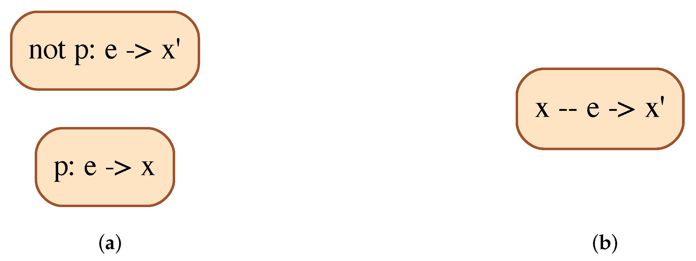
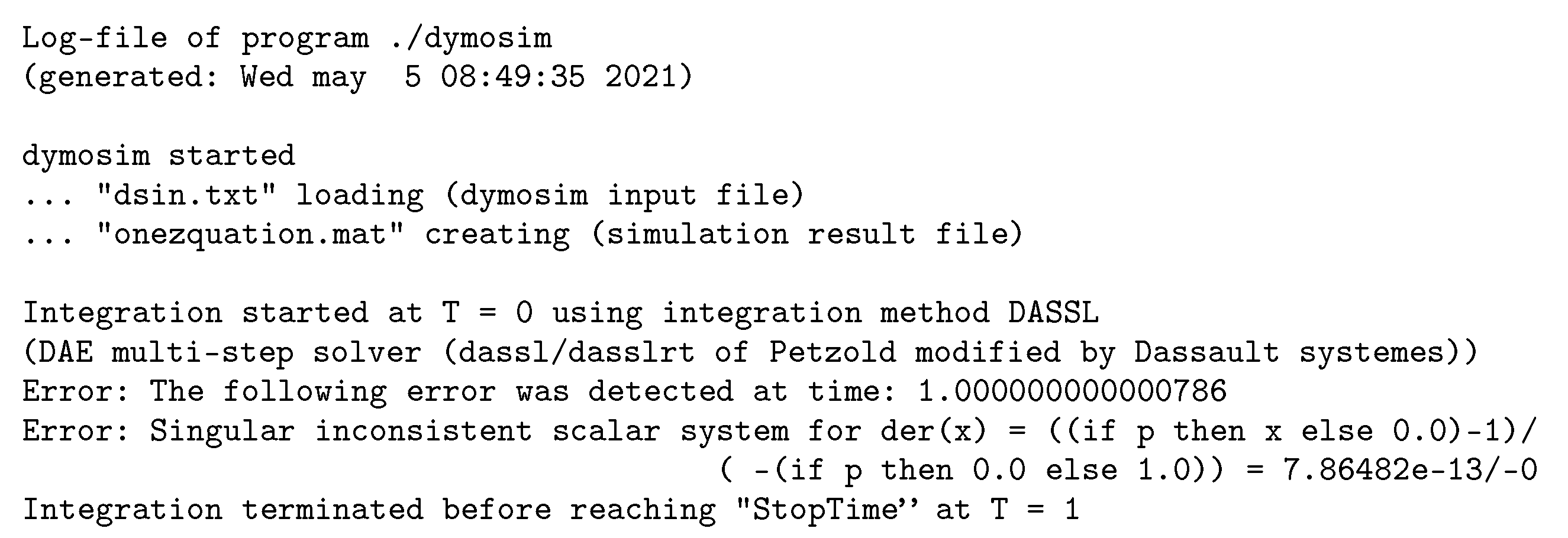

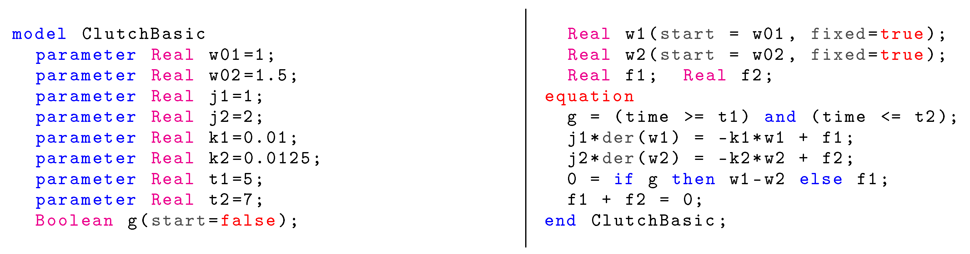
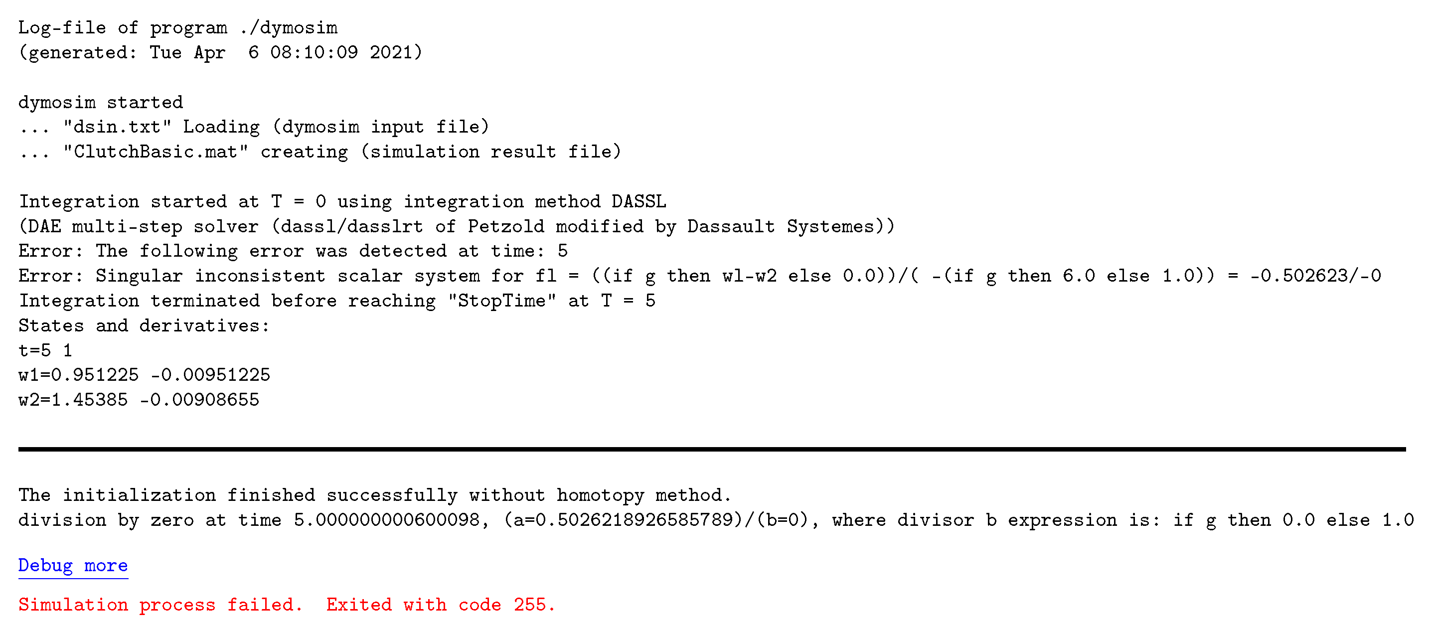
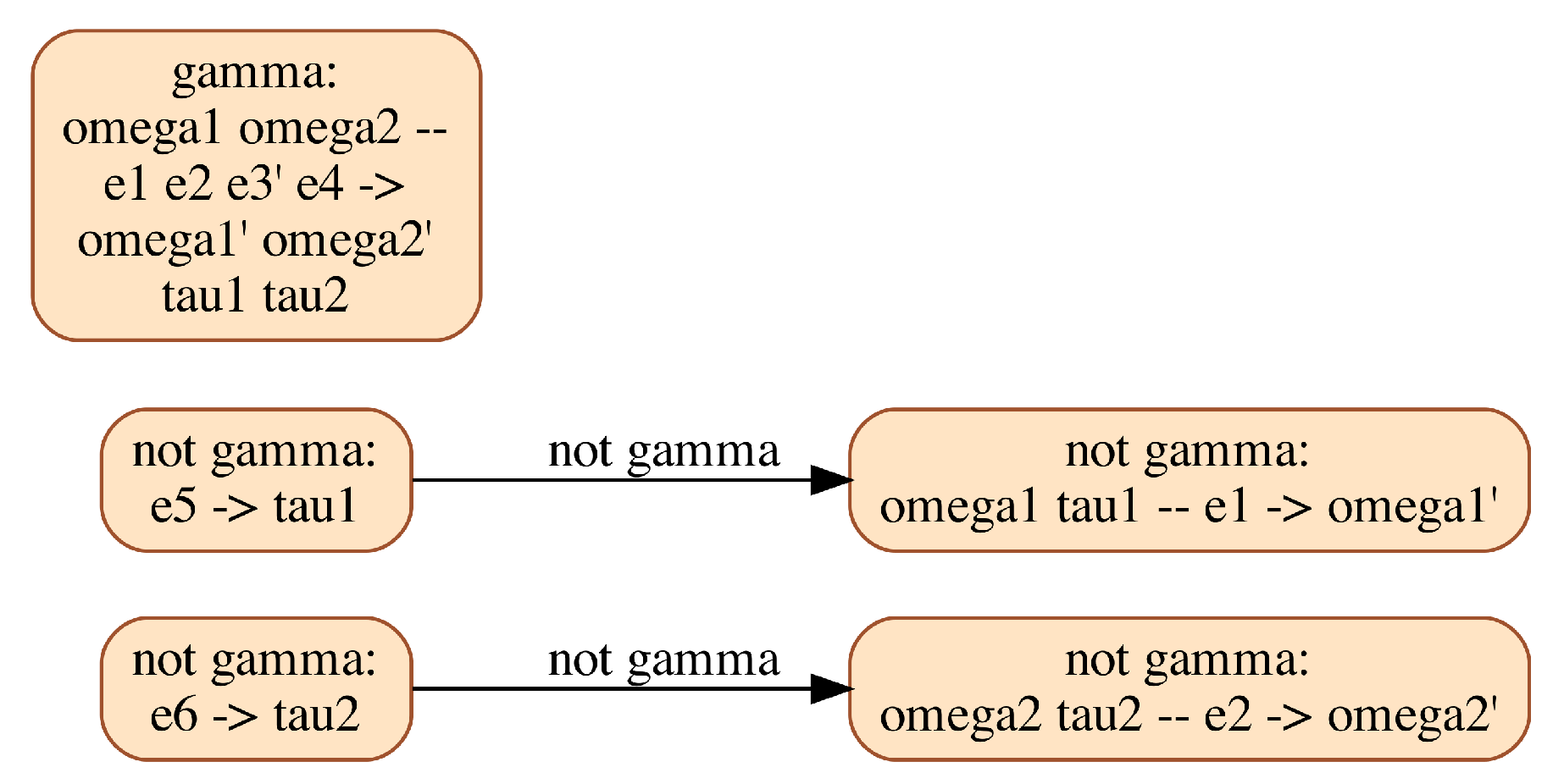
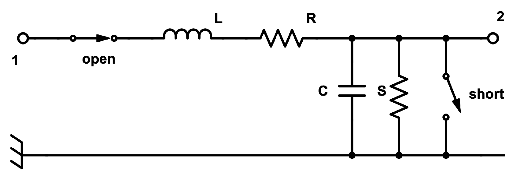
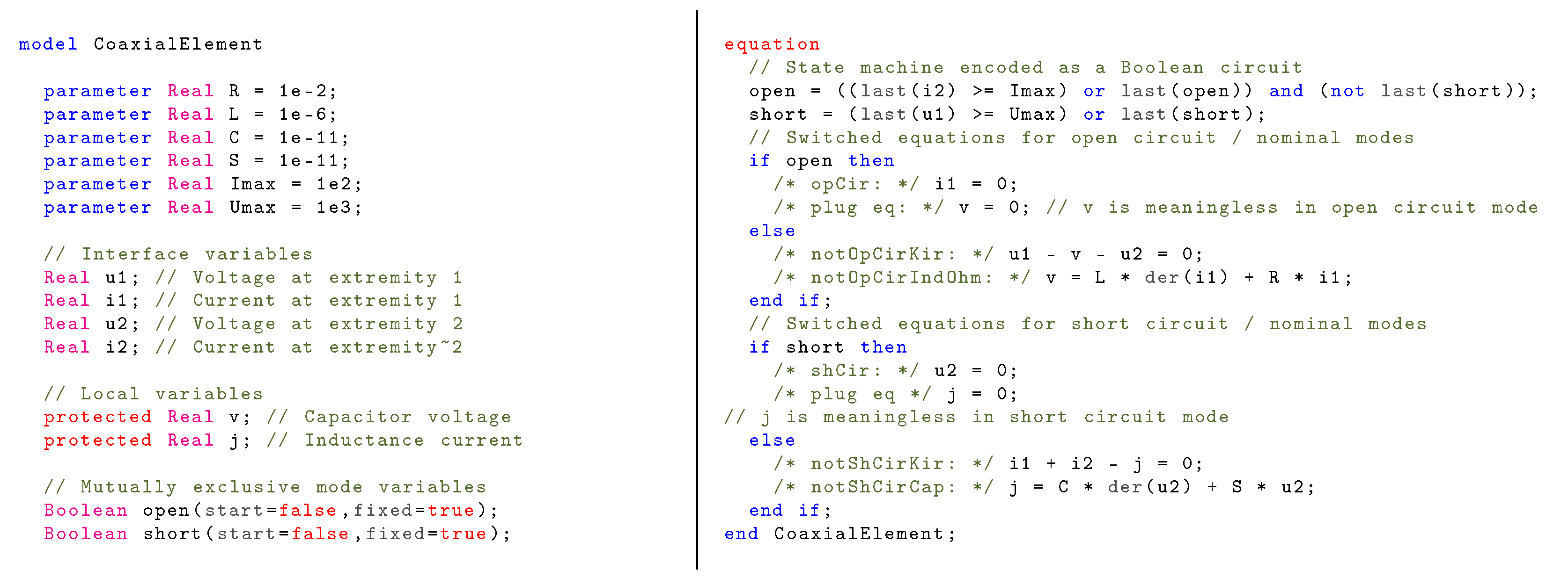
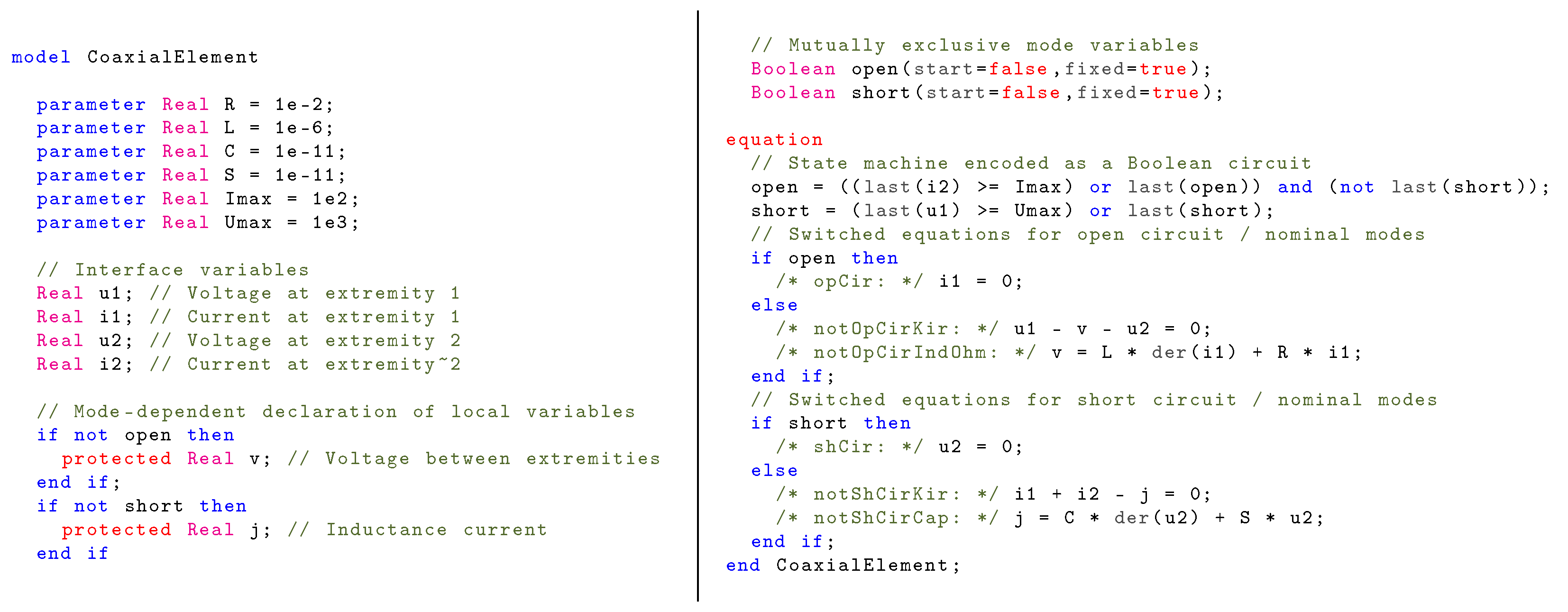
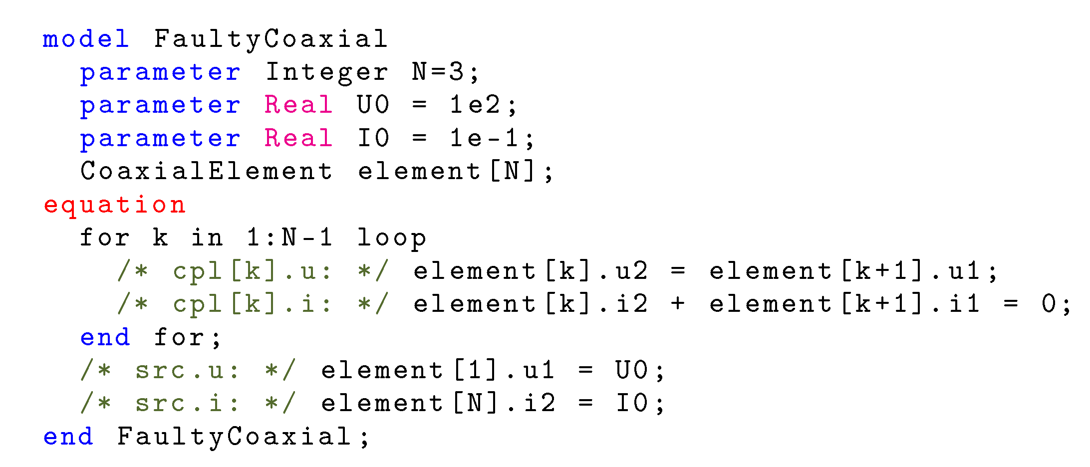
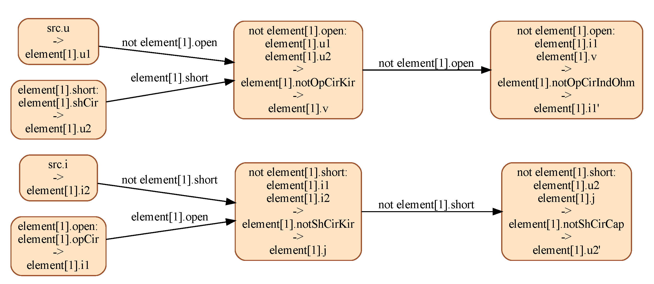

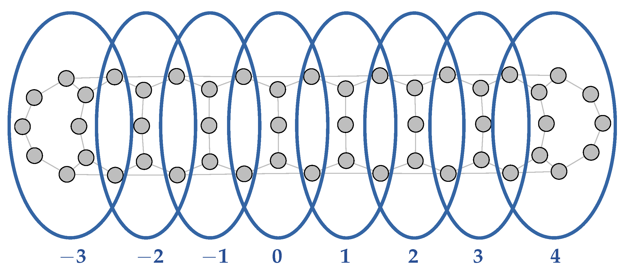
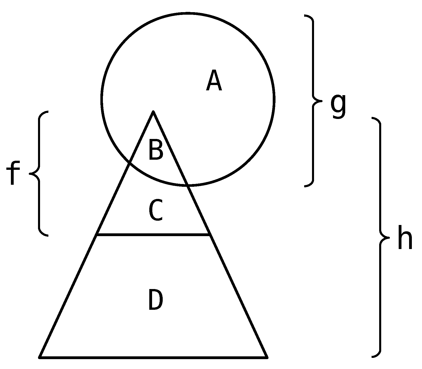
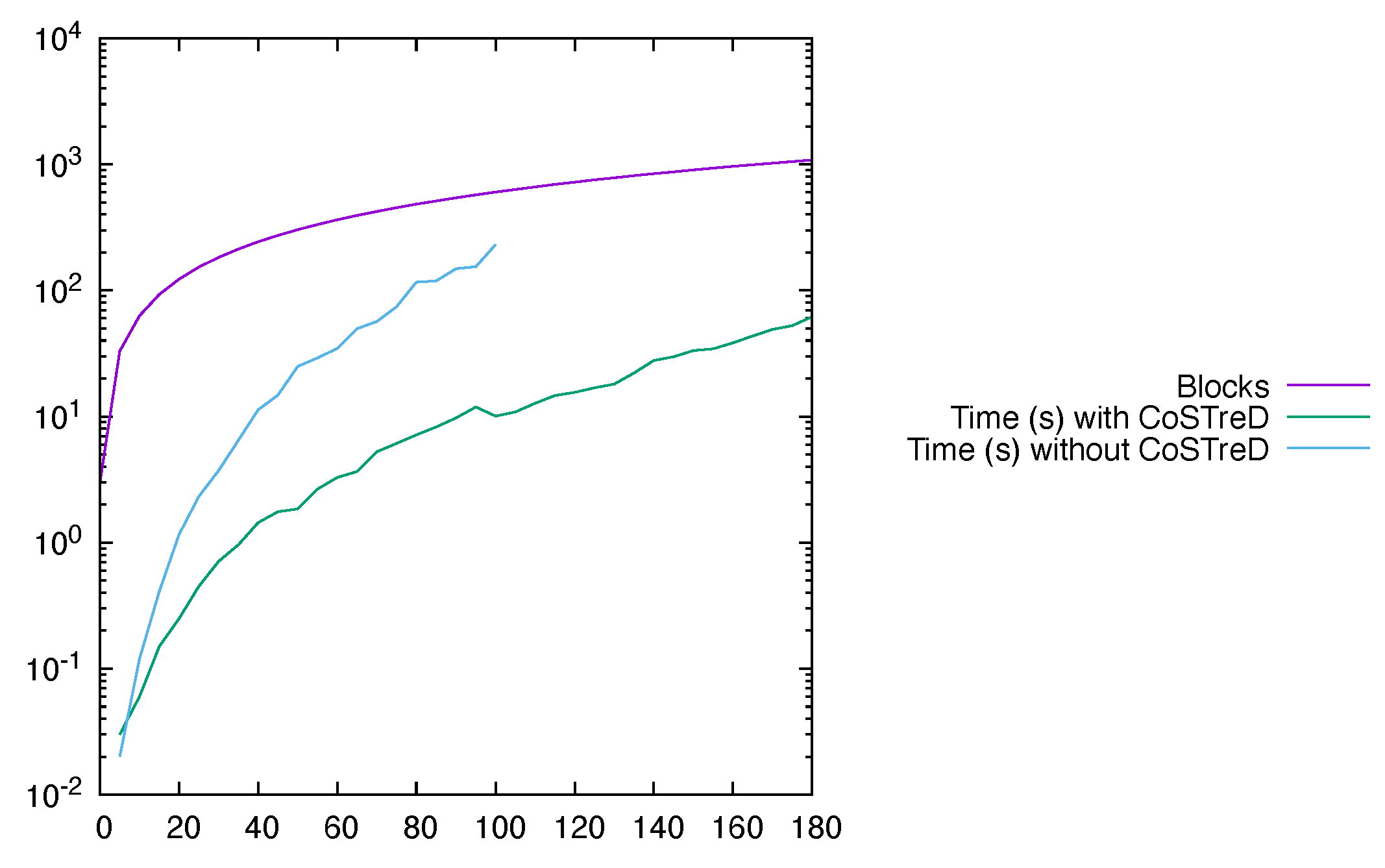
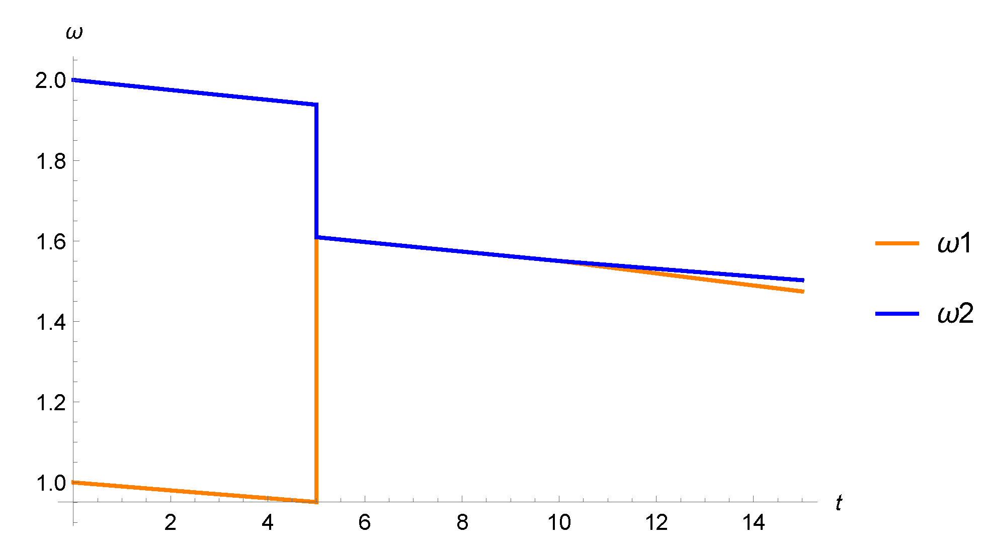

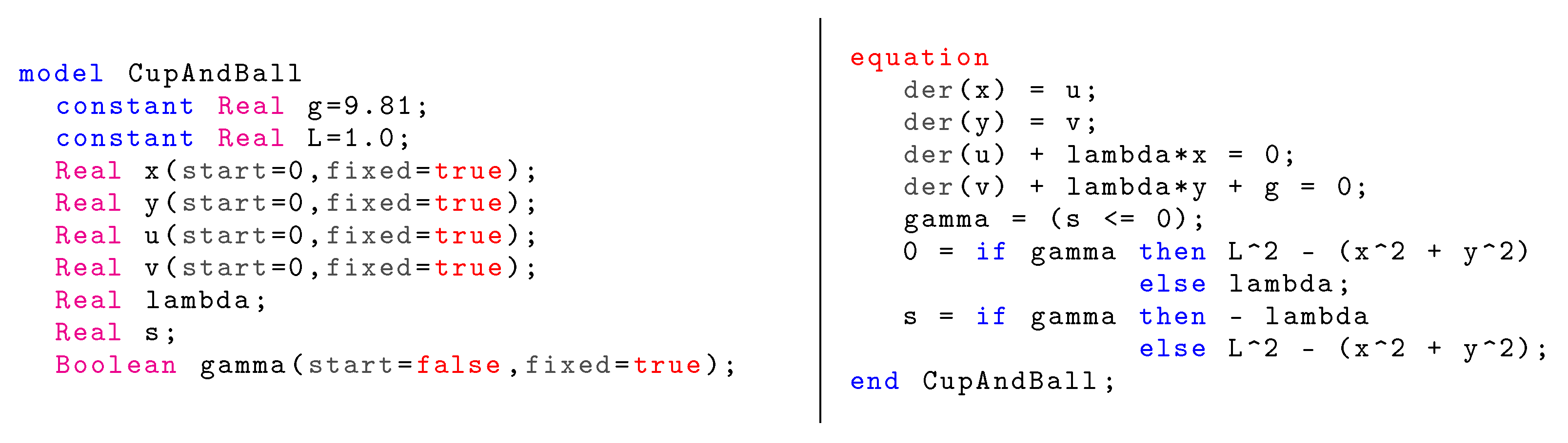
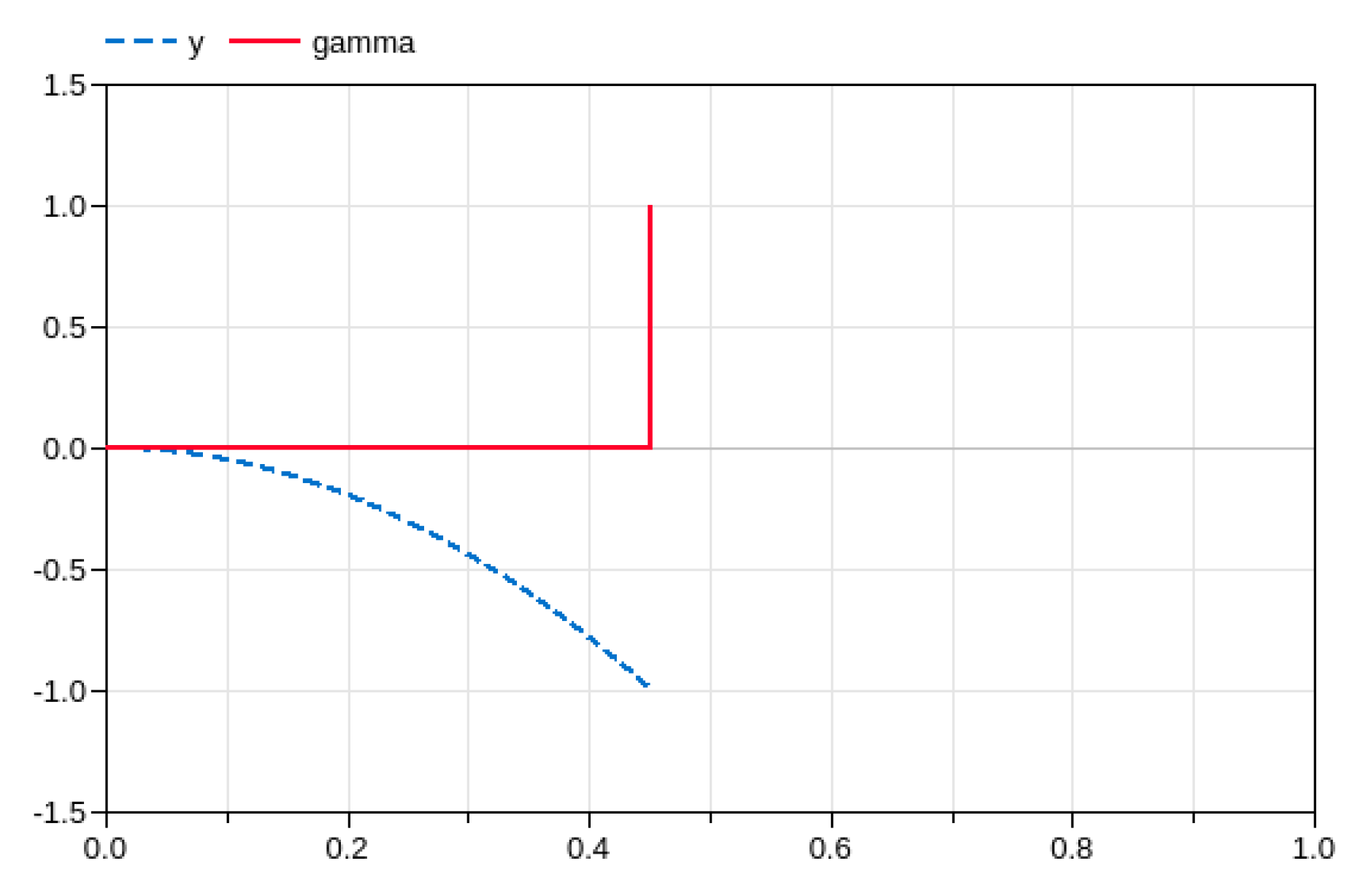


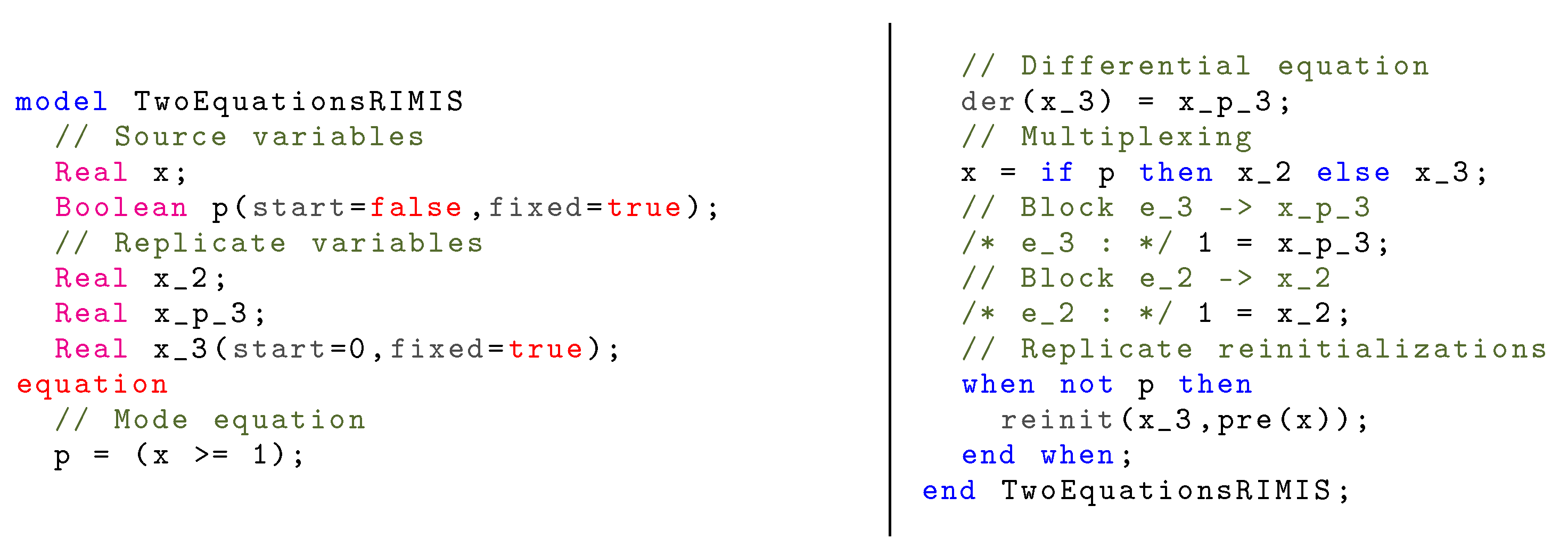
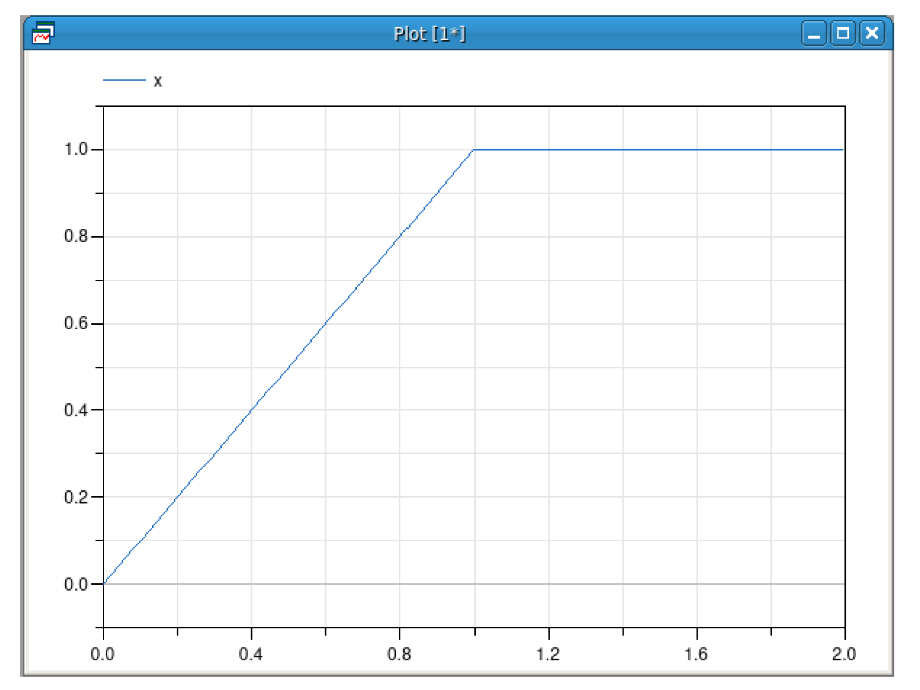
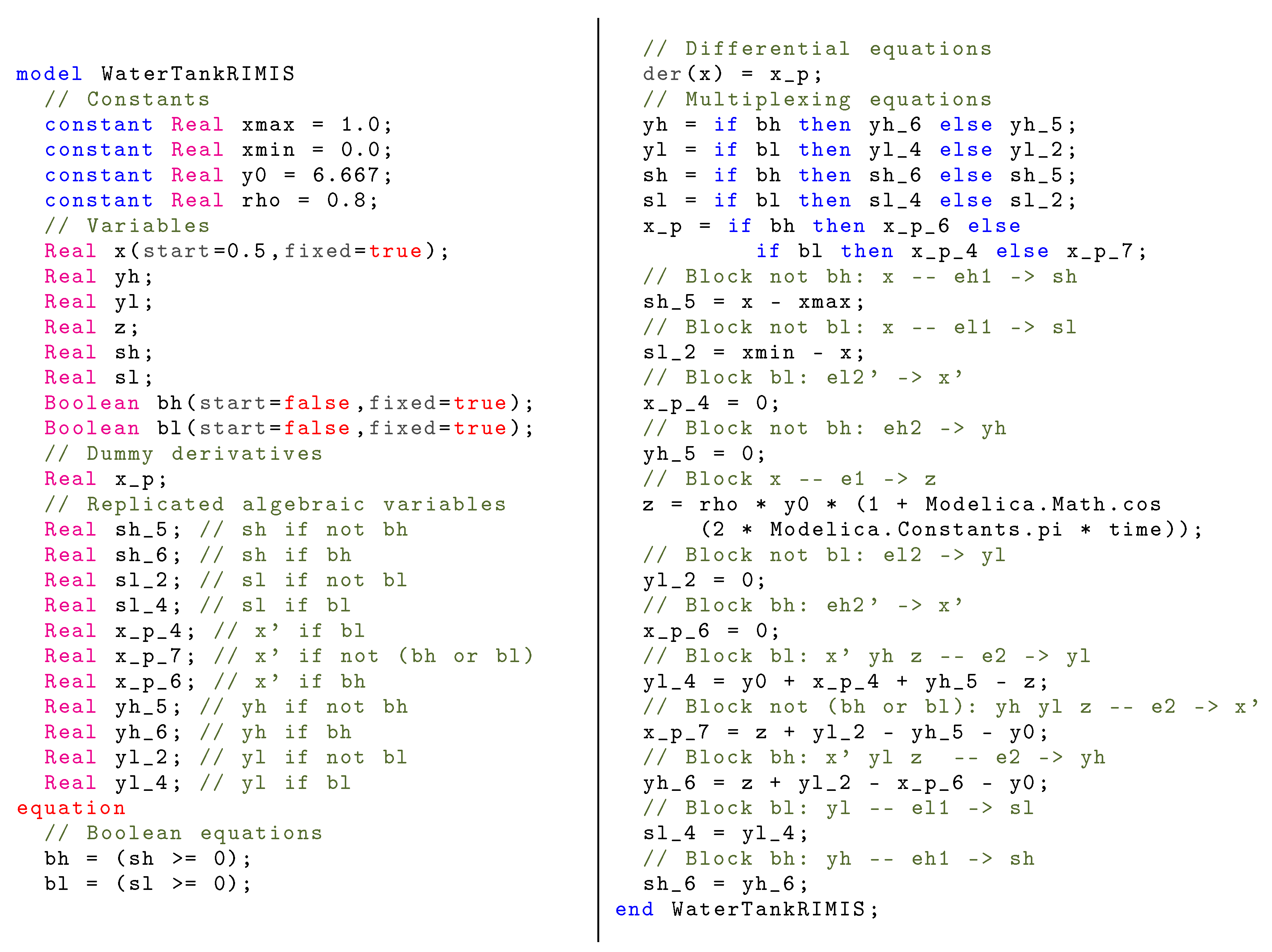
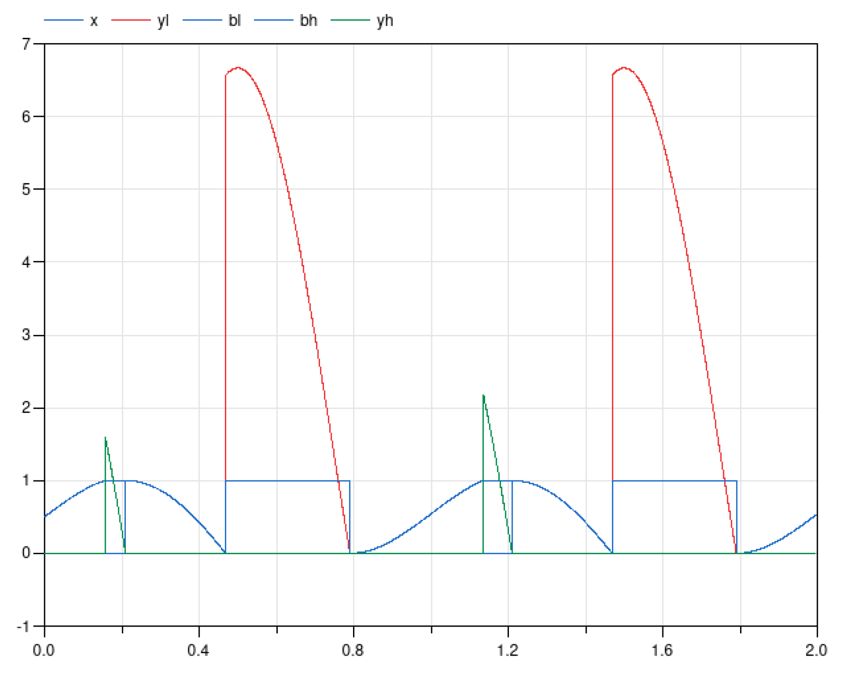
Publisher’s Note: MDPI stays neutral with regard to jurisdictional claims in published maps and institutional affiliations. |
© 2022 by the authors. Licensee MDPI, Basel, Switzerland. This article is an open access article distributed under the terms and conditions of the Creative Commons Attribution (CC BY) license (https://creativecommons.org/licenses/by/4.0/).