
GDR: A Game Algorithm Based on Deep Reinforcement Learning for Ad Hoc Network Routing Optimization


Abstract
:1. Introduction
- We apply game theory to the graph representation of routing engineering and pay attention to the performance of each node in the network in terms of energy consumption while ensuring network connectivity and efficiency;
- In view of the dynamic nature of the network, we train a network with reinforcement learning to achieve a near-optimal routing policy without prior information about the environment. It is worth pointing out that our input is a graph representation that is adapted by the game model, which is less computationally expensive and faster;
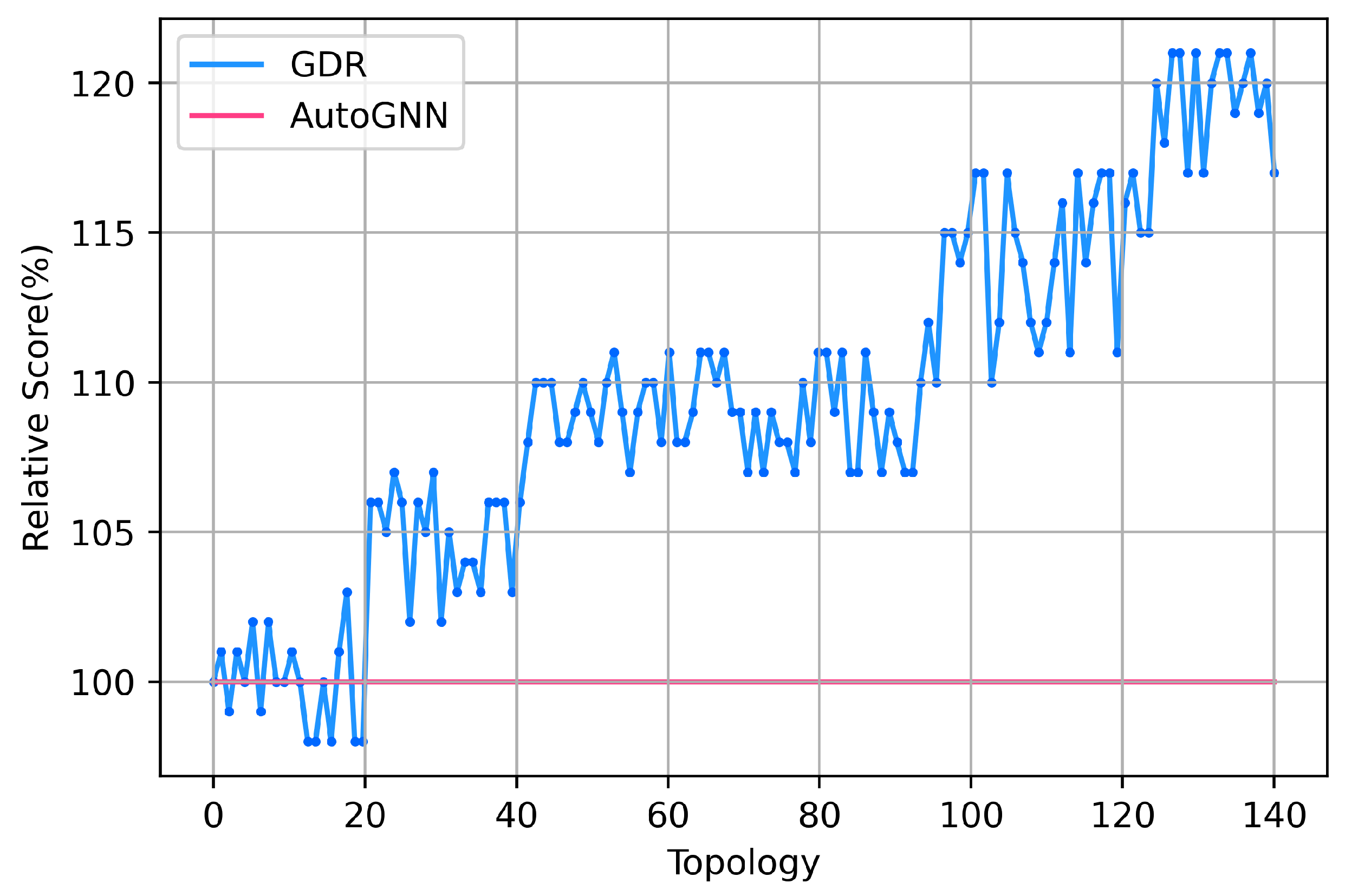
- We collect and experiment with network traffic data in the real world. The results show that the average end-to-end delay of GDR model is 10.5% higher than that of AutoGNN [14] on average. Meanwhile, the average lifespan of the network nodes is longer, the network energy consumption is more balanced, the energy efficiency of the entire network is improved, and the network structure is more robust.
2. Related Works
3. GDR Framework
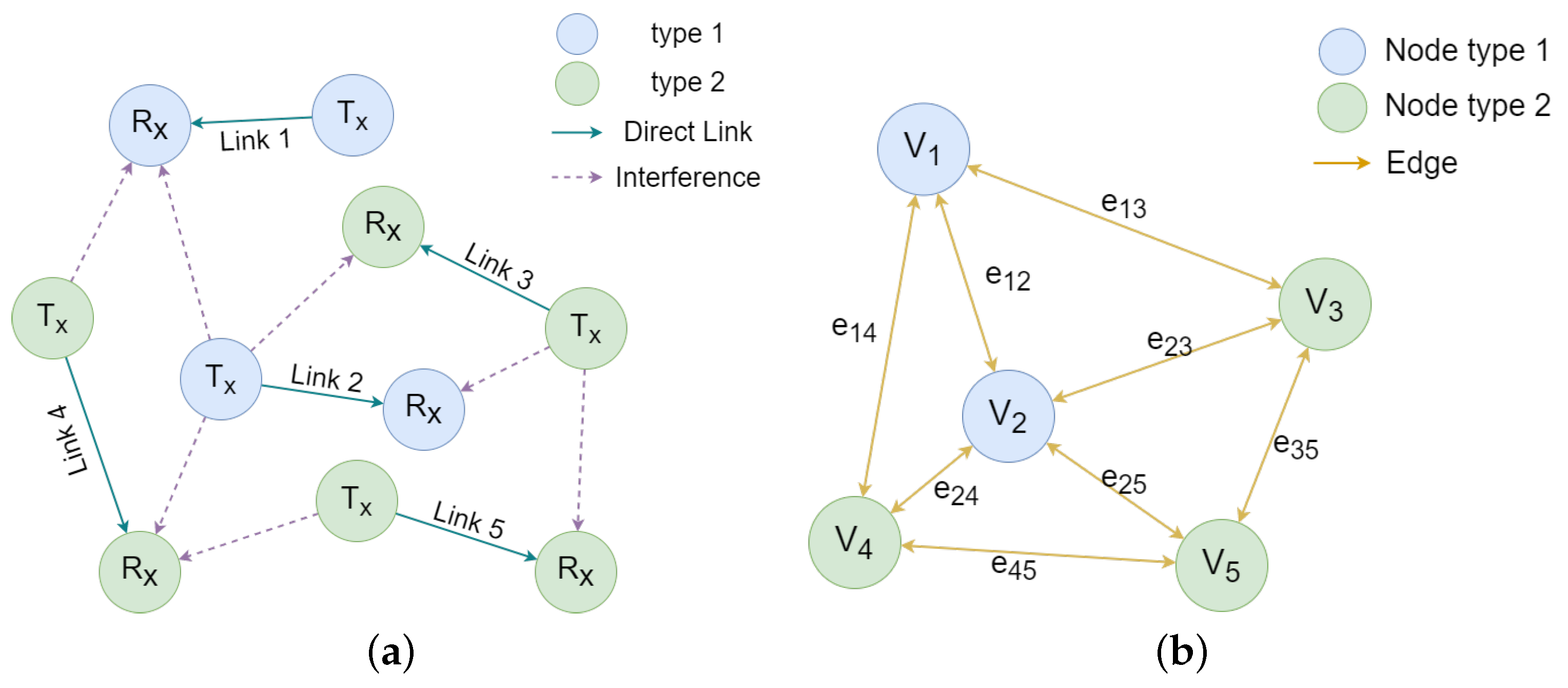
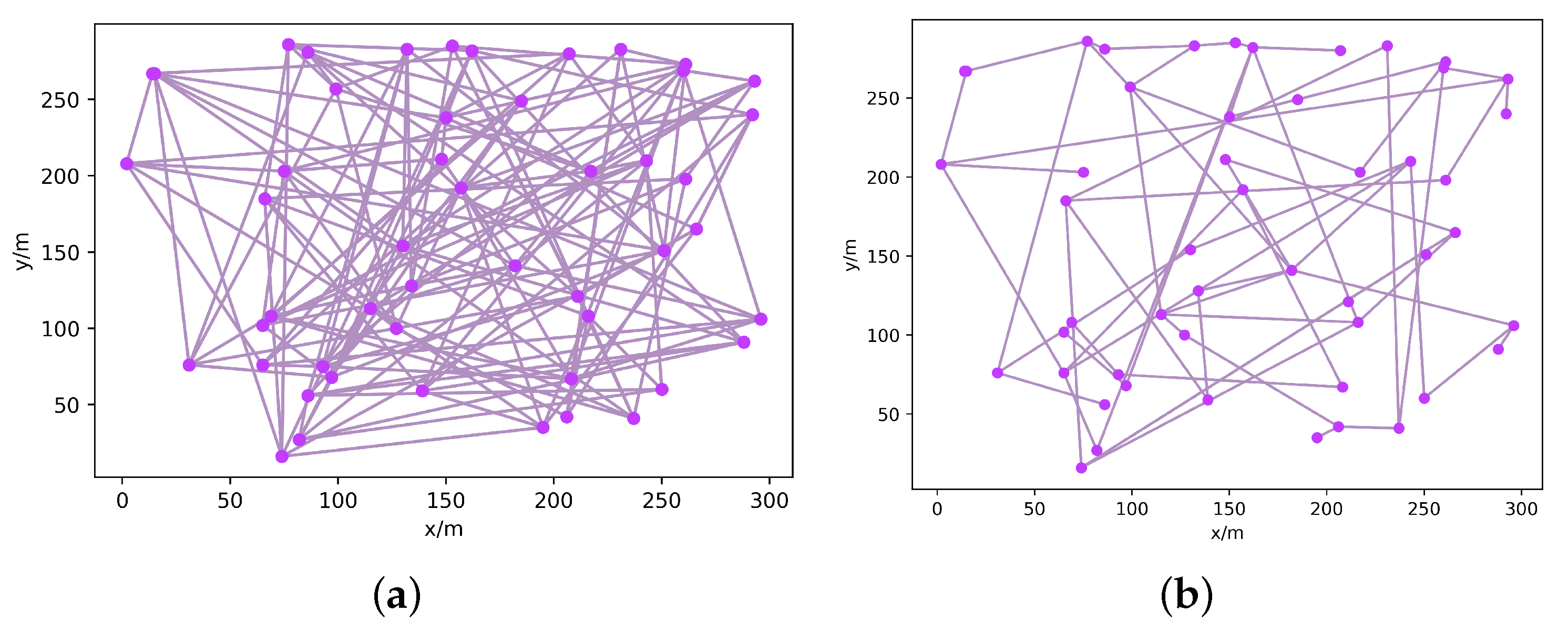
3.1. Dynamic Graph Construction for Ad Hoc Network
3.2. Game Algorithm for Topology Control
3.2.1. Game Model
3.2.2. Utility Function
3.2.3. Nash Equilibrium
| Algorithm 1 Topology Control Game Algorithm. |
|
3.3. GNN-Based DRL Agent
3.3.1. Deep Reinforcement Learning
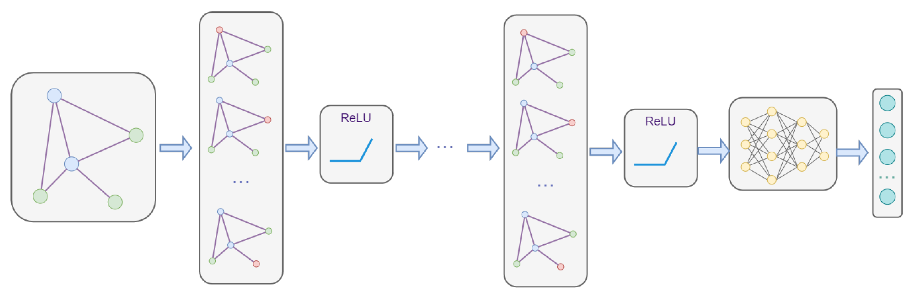
3.3.2. Graph Neural Networks
3.3.3. DRL Framework
- Agent: Based on the “GNN+DRL” framework, a central controller is considered as an agent, which means that our work uses a centralized reinforcement learning algorithm. The agent has the ability to learn and make decisions in the interaction with the environment. The central controller is responsible for performing routing optimization for the network;
- State: State in the reinforcement learning framework represents the information that the agent can obtain from the environment. This information is represented as a graph, including vertexes, edges and global information.
- Action: An action is a process of valid routing. Due to the dynamic nature of the Ad Hoc network, new incoming or outgoing nodes can cause changes in the state of the environment.
- Rewards: Instead of following predetermined labels, the learning agent optimizes the behavior of the algorithm by continuously obtaining rewards from the external environment. The principle of the “reward” mechanism is to tell the agent how comparatively good the current action is. In other words, the reward function directs the optimization direction of the algorithm. Accordingly, if we link the design of the reward function to the optimization goal, the performance of the system will be improved, driven by the rewards.
| Algorithm 2 DRL Agent Operation. |
|
4. Simulation and Evaluation
4.1. Simulation
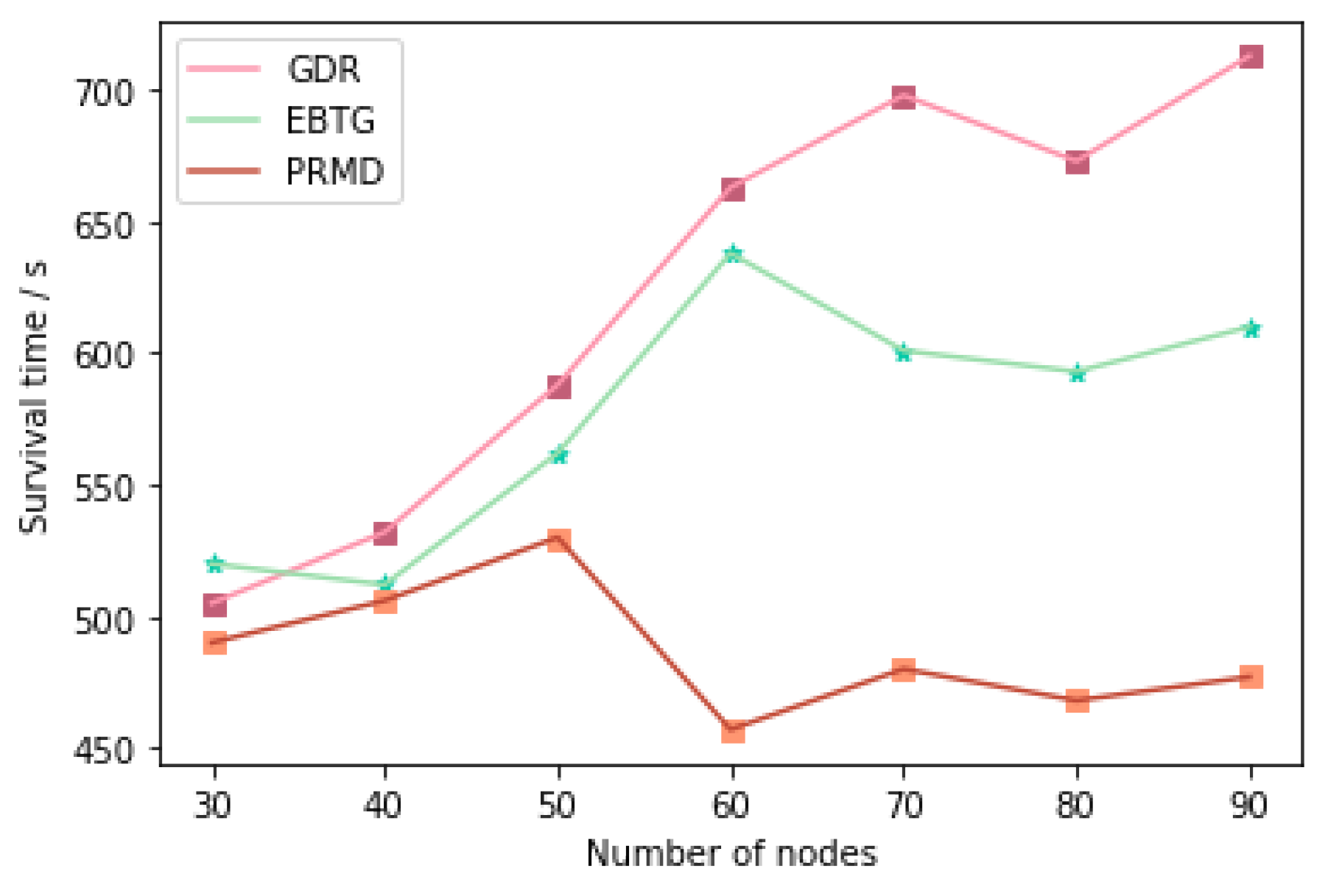
4.2. Evaluation
5. Conclusions
Author Contributions
Funding
Conflicts of Interest
References
- Ramanathan, R.; Rosales-Hain, R. Topology Control of Multiple Wireless Networks Using Transmit Power Adjustment. In Proceedings of the INFOCOM 2000. Nineteenth Annual Joint Conference of the IEEE Computer and Communications Societies, Tel Aviv, Israel, 26–30 March 2000. [Google Scholar]
- Zhao, J.; Dong, P.; Ma, X.; Sun, X.; Zou, D. Mobile-aware and relay-assisted partial offloading scheme based on parked vehicles in B5G vehicular networks. Phys. Commun. 2020, 42, 101163. [Google Scholar] [CrossRef]
- Du, Y.; Gong, J.; Wang, Z.; Xu, N. A distributed energy-balanced topology control algorithm based on a noncooperative game for wireless sensor networks. Sensors 2018, 18, 4454. [Google Scholar] [CrossRef] [PubMed]
- Du, Y.; Xia, J.; Gong, J.; Hu, X. An energy-efficient and fault-tolerant topology control game algorithm for wireless sensor network. Electronics 2019, 8, 1009. [Google Scholar] [CrossRef]
- Sun, P.; Hu, Y.; Lan, J.; Tian, L.; Chen, M. TIDE: Time-relevant deep reinforcement learning for routing optimization. Future Gener. Comput. Syst. 2019, 99, 401–409. [Google Scholar] [CrossRef]
- Tiwari, P.; Zhu, H.; Pandey, H.M. DAPath: Distance-aware knowledge graph reasoning based on deep reinforcement learning. Neural Netw. 2021, 135, 1–12. [Google Scholar] [CrossRef] [PubMed]
- Zhao, J.; Liu, J.; Yang, L.; Ai, B.; Ni, S. Future 5G-oriented system for urban rail transit: Opportunities and challenges. China Commun. 2021, 18, 1–12. [Google Scholar] [CrossRef]
- Wan, G.; Pan, S.; Gong, C.; Zhou, C.; Haffari, G. Reasoning like human: Hierarchical reinforcement learning for knowledge graph reasoning. In Proceedings of the Twenty-Ninth International Conference on International Joint Conferences on Artificial Intelligence, Yokohama, Japan, 7–15 January 2021; pp. 1926–1932. [Google Scholar]
- Suárez-Varela, J.; Mestres, A.; Yu, J.; Kuang, L.; Feng, H.; Cabellos-Aparicio, A.; Barlet-Ros, P. Routing in optical transport networks with deep reinforcement learning. J. Opt. Commun. Netw. 2019, 11, 547–558. [Google Scholar] [CrossRef]
- Albawi, S.; Mohammed, T.A.; Al-Zawi, S. Understanding of a convolutional neural network. In Proceedings of the International Conference on Engineering and Technology (ICET), Antalya, Turkey, 21–23 August 2017; pp. 1–6. [Google Scholar]
- Zaremba, W.; Sutskever, I.; Vinyals, O. Recurrent neural network regularization. arXiv 2014, arXiv:1409.2329. [Google Scholar]
- Zhu, T.; Chen, X.; Chen, L.; Wang, W.; Wei, G. Gclr: Gnn-based cross layer optimization for multipath tcp by routing. IEEE Access 2020, 8, 17060–17070. [Google Scholar] [CrossRef]
- You, X.; Li, X.; Xu, Y.; Feng, H.; Zhao, J.; Yan, H. Toward Packet Routing with Fully-distributed Multi-agent Deep Reinforcement Learning. IEEE Trans. Syst. Man Cybern. Syst. 2019, 52, 855–868. [Google Scholar] [CrossRef]
- Chen, B.; Zhu, D.; Wang, Y.; Zhang, P. An Approach to Combine the Power of Deep Reinforcement Learning with a Graph Neural Network for Routing Optimization. Electronics 2022, 11, 368. [Google Scholar] [CrossRef]
- Scarselli, F.; Gori, M.; Tsoi, A.C.; Hagenbuchner, M.; Monfardini, G. The graph neural network model. IEEE Trans. Neural Netw. 2008, 20, 61–80. [Google Scholar] [CrossRef] [PubMed]
- Naderializadeh, N.; Eisen, M.; Ribeiro, A. Wireless power control via counterfactual optimization of graph neural networks. In Proceedings of the IEEE 21st International Workshop on Signal Processing Advances in Wireless Communications (SPAWC), Atlanta, GA, USA, 26–29 May 2020; pp. 1–5. [Google Scholar]
- Zhao, D.; Qin, H.; Song, B.; Han, B.; Du, X.; Guizani, M. A graph convolutional network-based deep reinforcement learning approach for resource allocation in a cognitive radio network. Sensors 2020, 20, 5216. [Google Scholar] [CrossRef]
- Zhang, X.; Zhao, H.; Xiong, J.; Liu, X.; Zhou, L.; Wei, J. Scalable power control/beamforming in heterogeneous wireless networks with graph neural networks. In Proceedings of the IEEE Global Communications Conference (GLOBECOM), Madrid, Spain, 7–11 December 2021; pp. 1–6. [Google Scholar]
- Wang, H.; Qiu, Z.; Dong, R.; Jiang, H. Energy balanced and self adaptation topology control game algorithm for wireless sensor networks. Kongzhi yu Juece/Control Decis. 2019, 34, 72–80. [Google Scholar]
- Yang, S.; Lian-Suo, W.; Yuan, G. Multi-Objective Fusion Ordinal Potential Game Wireless Ad Hoc Network Topology Control Algorithm. J. Beijing Univ. Posts Telecommun. 2022, 105–111. [Google Scholar]
- Kao, S.C.; Yang, C.H.H.; Chen, P.Y.; Ma, X.; Krishna, T. Reinforcement learning based interconnection routing for adaptive traffic optimization. In Proceedings of the 13th IEEE/ACM International Symposium on Networks-on-Chip, New York, NY, USA, 17–18 October 2019; pp. 1–2. [Google Scholar]
- Kaur, A.; Kumar, K. Energy-efficient resource allocation in cognitive radio networks under cooperative multi-agent model-free reinforcement learning schemes. IEEE Trans. Netw. Serv. Manag. 2020, 17, 1337–1348. [Google Scholar] [CrossRef]


| Parameter | Value |
|---|---|
| Number of initial nodes | 50 |
| Initial energy of node | 50 J |
| cell radius | 100 m |
| system loss | 1 |
| Wave length | 0.1224 m |
| Monitoring area | 300 × 300 m2 |
| Node residual energy | The Poisson distribution that obeys of 25 |
| SP | CNN+DRL | GMM | AutoGNN [14] | GDR | |
|---|---|---|---|---|---|
| Neural networks | GNN | CNN | ✘ | GNN | GNN |
| DRL framework | ✘ | ✔ | ✘ | ✔ | ✔ |
| Convergence time | 6000 s | ⩾60,000 s | ✘ | 48,000 s | 25,000 s |
| Optimal solution | ✘ | ✘ | ✘ | ✔ | ✔ |
| Scalability | ✘ | ✘ | ✔ | ✔ | ✔ |
Publisher’s Note: MDPI stays neutral with regard to jurisdictional claims in published maps and institutional affiliations. |
© 2022 by the authors. Licensee MDPI, Basel, Switzerland. This article is an open access article distributed under the terms and conditions of the Creative Commons Attribution (CC BY) license (https://creativecommons.org/licenses/by/4.0/).
Share and Cite
Hong, T.; Wang, R.; Ling, X.; Nie, X. GDR: A Game Algorithm Based on Deep Reinforcement Learning for Ad Hoc Network Routing Optimization. Electronics 2022, 11, 2873. https://doi.org/10.3390/electronics11182873
Hong T, Wang R, Ling X, Nie X. GDR: A Game Algorithm Based on Deep Reinforcement Learning for Ad Hoc Network Routing Optimization. Electronics. 2022; 11(18):2873. https://doi.org/10.3390/electronics11182873
Chicago/Turabian StyleHong, Tang, Ruohan Wang, Xiangzheng Ling, and Xuefang Nie. 2022. "GDR: A Game Algorithm Based on Deep Reinforcement Learning for Ad Hoc Network Routing Optimization" Electronics 11, no. 18: 2873. https://doi.org/10.3390/electronics11182873