Abstract
The navigation performance of an autonomous underwater vehicle (AUV) as the main tool for exploring the ocean greatly affects its work efficiency. Under the circumstance that high-precision GNSS positioning signals cannot be obtained, the role of the Strapdown Inertial Navigation System/Doppler Velocity Log (SINS/DVL) integrated navigation system is becoming more prominent. Due to marine creatures or the seafloor topography, DVL is prone to outliers or even failures during measurement. To solve these problems, a LSTM/SVR-VBAKF algorithm aided integrated navigation system is proposed. First, under normal circumstances of DVL, the output information of SINS and DVL are used as training samples, and they train the Long Short-Term Memory (LSTM) model. To enhance the robustness and adaptability of the filter, a novel variational Bayesian adaptive filtering algorithm based on support vector regression is proposed. When the DVL formation is missing, the deep learning method adopted in this paper will be continuously output to ensure the effect of integrated navigation. The shipboard test data is verified from two aspects: filter performance and neural network-assisted integrated navigation system capability. The experimental results show that the new method proposed in this paper can effectively handle a situation where DVL output is not available.
1. Introduction
As an important tool in the process of human exploration of the ocean, AUV has an important function in resource exploration and environmental investigation. In order to facilitate the operation of underwater vehicles, high-precision underwater navigation and positioning technology is essential. Different from the surface and terrestrial environments, the radio signals in the underwater environment decay rapidly, and traditional radio navigation methods, such as GNSS, cannot provide effective and safe navigation information for underwater vehicles [1]. Strap-down Inertial Navigation System (SINS), as an effective tool for providing attitude, velocity, and position information, can provide navigation information autonomously, and it has the advantages of small size, light weight, and easy maintenance [2]. It has been used on various types of underwater vehicles. It is undeniable that, as a navigation method according to the traditional Newton’s law, its attitude error and velocity error oscillate periodically, and the position error keeps accumulating deviation. At present, in addition to inertial navigation in the underwater environment, with the diversification of detection methods, geophysical navigation, acoustic navigation, collaborative navigation, and other methods have emerged as required by time [3,4]. Geophysical navigation mainly uses the characteristics of geophysical parameters (topography, gravitational field, magnetic field) to obtain the current position information of the vehicle [5]. This method has high navigation accuracy and is not limited by regions, but it is limited by the accuracy and stability of the sensor, so it is not widely used at present [6]. Acoustic navigation uses the reference position information provided by the hydrophone, which measures the time when the pulse signal sent by the vehicle reaches the reference position and then provides the current position information [7]. However, the transducer needs to be placed in advance, which limits the navigation range. Cooperative navigation uses underwater acoustic communication technology to share measurement information and to coordinate the distance and relative position information of each vehicle [8]. At present, cooperative navigation is in the stage of theoretical research and verification. The various advantages and disadvantages of the current underwater navigation methods cannot meet the growing demand of underwater vehicles, so the integrated navigation method has become mainstream. The common underwater integrated navigation method is SINS/DVL [9,10]. This method takes SINS as the main body, and performs data fusion processing according to the three-dimensional velocity of underwater vehicle measured by DVL so as to meet the requirements of improving navigation and positioning accuracy. The size of the navigation system increases, which contributes to the increase in complexity, so the probability of system failure increases. For underwater vehicles, the complex ocean environment, such as ocean current interference, terrain changes, and sudden encounters with marine creatures, the large angle motion of underwater vehicles will affect the output of DVL, resulting in outliers or even output interruption [11]. When the DVL output is abnormal, if only traditional inertial navigation methods are used, the errors will inevitably accumulate, and it is impossible to achieve high-precision underwater positioning. Therefore, the research on the DVL failure treatment method for underwater vehicles is of great significance for underwater high-precision positioning.
The failure processing method for DVL can be solved from two levels: hardware structure and software algorithm. In terms of hardware, by designing multiple sets of parallel navigation sensors, when one of the sensors failed, it can be replaced by the other [12], but it will increase the complexity and cost of the system. In order to save costs, scientists began to consider this problem from the software level. The first is a method based on vehicle kinetic model information to assist SINS [13]. Although the prediction of DVL velocity can be achieved, the performance of integrated navigation is degraded. With the development of various deep learning theories, alternative methods have gradually increased when DVL fails. A new extended loose coupling method (ELC), which combined the original DVL information and external additional information to provide virtual vehicle motion information was proposed by [14]; it used simulation software to perform six-degree-of-freedom test verification. Besides, replacing failed DVL sensor outputs with deep learning modules is emerging, e.g., Radial Basis Function Neural Network (RBFNN) [15] and Least Squares Support Vector Machine algorithm (LSSVM) [16]. They have a common disadvantage in that they cannot effectively utilize past dynamic information. Nonlinear Autoregressive Neural Network (NARX) with external input as a dynamic neural network can solve this problem [17,18], but they ignore the associations of input and output during training and two SINS loops complicate the structure. Fuzzy rules are used by [19,20] to construct pseudo-measurements. This undoubtedly complicates the learning of the system.
In addition, DVL also has the problem of abnormal measurement value in the measurement process. Compared to issues that fail for a period of time, if “pseudo-sensors”, such as neural networks are used, there may be problems, such as low reliability of training results due to inaccurate data. However, the appearance of such outliers can be handled in the information fusion stage, that is to enhance the robustness of the filter. There are many methods for robustness of current filters: ref. [21] combines SHAKF methods with variable sliding windows and decay filters; the improved robust Kalman filter proposed by [22] constructs the cost function according to the statistical similarity measure (SSM), and optimizes it; ref. [23] designed a traditional chi-square test assisted two-factor adaptive filter; refs. [24,25] use the maximum entropy criterion to robustly process the Kalman filter; and ref. [26] discriminated and detected outliers based on Mahalanobis distance and introduced an attenuation factor to scale outliers to improve anti-interference capability of the filter. The above robust methods are all carried out in the filtering framework, which may lead to a large amount of calculation and singular values in matrix decomposition. The Gaussian process regression method was introduced into the Kalman filter by [27], which can detect outliers faster than the chi-square test method. However, this method is only used to detect outliers, and the selection of the threshold value is based on experience. A fuzzy neural network with optimized coefficients and a maximum entropy Kalman filter was combined by [28] to deal with non-Gaussian noise by adaptively adjusting the bandwidth coefficient.
To solve the problem of DVL failure in AUV motion, this paper proposes a hybrid prediction method combining long-short-term memory neural network (LSTM) and machine learning method assisted adaptive filtering algorithm. The method can effectively solve the problems of DVL failure and inability to provide measurement values and outlier interference in the DVL measurement process. Especially in the construction of “pseudo-measurement value”, the original navigation information generated and measured by the SINS, which is directly related to the three-dimensional velocity measured by the DVL, is used as the training set, e.g., attitude, velocity, gyroscope, and accelerometer output. The navigation increment information calculated by the traditional inertial navigation solution is not directly used as the training set. To avoid introducing sensor errors, the output of the deep learning model is directly in the form of a DVL output. At the same time, the SVR method can also avoid the introduction of abnormal sample data when the deep learning model collects training samples. The experimental results show that LSTM/SVR-VBAKF algorithm proposed in this paper can not only effectively provide measurement values for the SINS/DVL integrated navigation system when the DVL fails but also avoid the influence of outliers and effectively improve the accuracy of navigation.
The remaining structure of this paper is as follows. Section 2 introduces each coordinate system of the strapdown inertial navigation system, as well as the state equation and measurement equation of the SINS/DVL integrated navigation system. In Section 3, a new adaptive filter assisted by the SVR method is proposed. Section 4 introduces the basic principle of the deep learning method and the specific steps of continuous integrated navigation using the deep learning model. In the Section 5, a river test is designed to illustrate the performance of the method. Finally, the corresponding conclusions are reached in Section 6.
2. SINS/DVL Integrated Navigation System Model
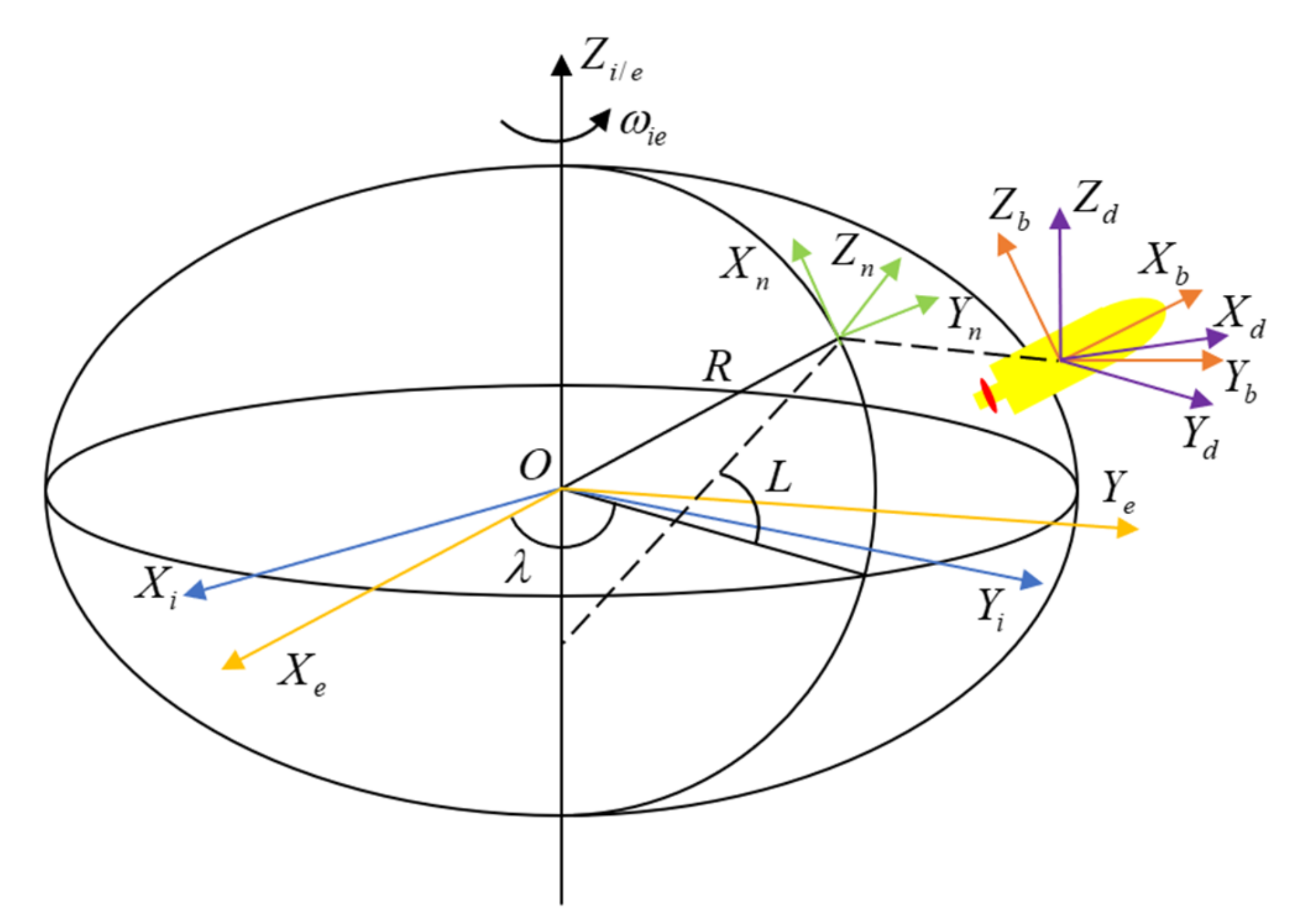
All parameters in SINS are expressed in different specific frames, and the exchange between different frames are frequent [29]. Therefore, the coordinate system used in this paper is first given here. In this paper, the common coordinate systems are as follows: the inertial frame is denoted by i, b represents the body frame of the SINS, the coordinate system used for navigation parameter calculation is defined by n, its orientation is east-north-up (ENU). The instrumental frame of DVL is denoted by d. During the process of integrated navigation, the IMU output carrier acceleration and angular velocity under b reference frame converts them to navigation parameters under the n reference frame through attitude conversion and integral operation. The velocity information output by DVL is usually in the reference frame d containing the installation angle errors. Therefore, it is necessary to transform d reference frame into n reference frame for attitude transformation. Specific reference frames are depicted in Figure 1.
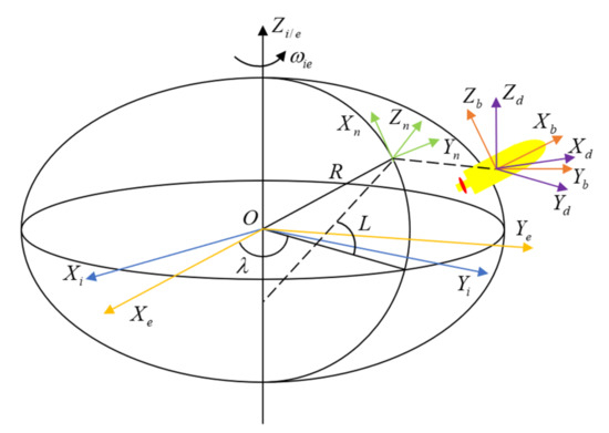
Figure 1.
Schematic diagrams of various commonly used reference frames.
2.1. State Equation of SINS/DVL Integrated Navigation System
Formula (1) gives the linear SINS error model [30].
where the , , , , . Reference [22] gives the meanings of the above error parameters. represents the rotation velocity of the earth, the rotational angular velocity of the earth system relative to the navigation system, and . denotes the transformation matrix. and represent the corresponding rotational angular velocity error term. and represent the basic data output by inertial devices for navigation solving. represents the influence of gravity on the accuracy of navigation system.
The state space model of a traditional integrated navigation system is usually composed of various error parameters of SINS. Since the installation angle error between SINS and DVL, the scale factor of DVL, and the installation lever error can be done in the calibration process, they can be ignored [31]. The state variables of the integrated navigation system are selected as 15 dimensions. The state variables are as in Formula (2).
The traditional system state space model is usually composed of Formula (3).
In Formula (3), F represents the system state transition matrix and W is the state noise. Ref. [32] provides their specific definitions.
2.2. Observation Space Model of SINS/DVL Integrated Navigation System
It has been explained in the previous section that the DVL measures the velocity in the d reference frame. In order to perform information fusion, the frame must be transformed. The following formula gives the transformation relation as Formula (4)
The above two attitude transformation matrices can be obtained by Formula (5).
where I represents the unit matrix of , represents the errors during device installation. It can be compensated in advance [33]. By merging the above two equations. We can obtain Formula (6).
Under normal circumstances, the measurement of integrated navigation system usually uses the difference between two velocity sensors as input, and its form can be expressed by the following Formula (7).
where H represents the observability matrix and V represents its noise. The specific form of the measurement matrix is as follows in Formula (8).
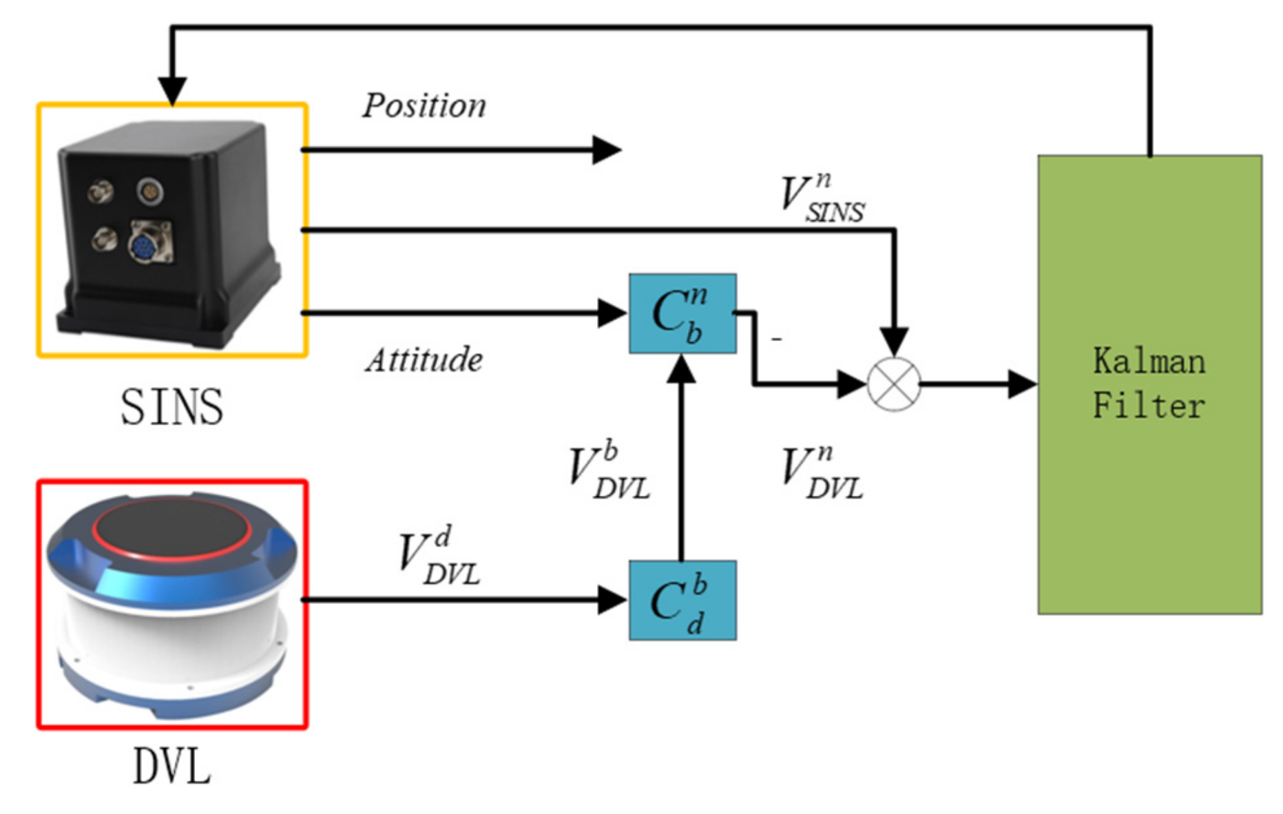
The specific integrated navigation system schematic diagram is shown by Figure 2 below:

Figure 2.
Schematic diagram of the principle of the integrated navigation system.
3. Principle of Adaptive Filter Assisted by Machine Learning Method
3.1. The Basical Principle of SVR
The support vector machine itself was used to solve the classification problem of the hyperplane, and it is also widely used in the field of data regression, that is, SVR. For the traditional training set , , . Its fitting function is shown in Formula (9) [34,35,36].
All parameters of Formula (9) can be obtained by reference [34]. The objective function and constraints of the SVR model are as follows.
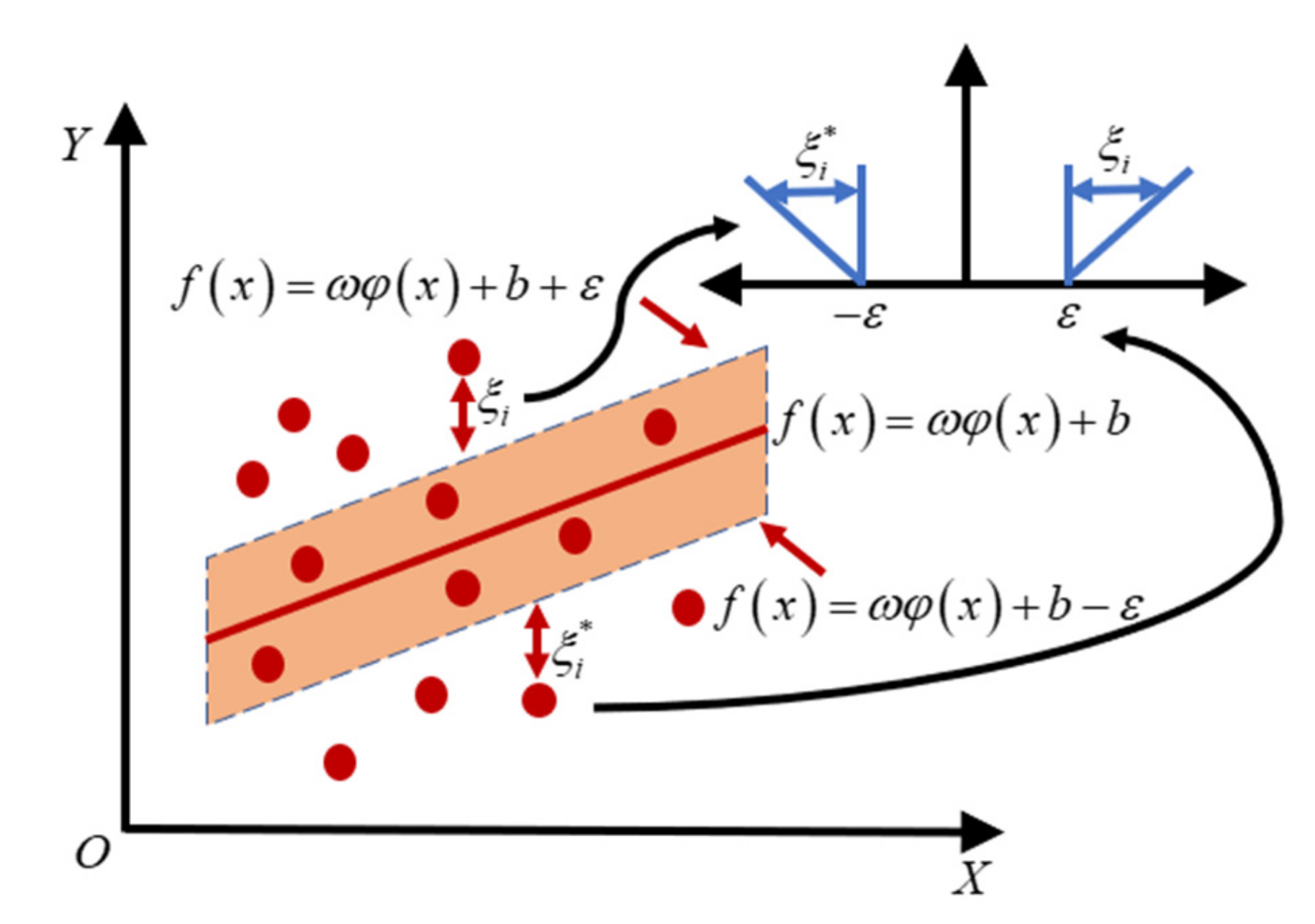
In Formula (10), is the insensitivity coefficient, C is the penalty factor, which influences the degree of penalty for the samples exceeding the error; the larger, the better the regression effect but the worse its generalization ability, is the relaxation factor. It can be solved by the following Formula (11):
In Formula (11), represents the multipliers. Because of the KKT condition, the optimal solution is calculated and sorted to obtain the final regression function expression, and a kernel function that conforms to the Mercer condition is introduced.
In Formula (12), is to complete space transformation efficiently. At present, there are many kinds of kernel functions to choose from, but the most commonly used is Gaussian radial basis function (RBF), which has good performance for large or small samples. Moreover, compared with the polynomial kernel function, it has fewer parameters and has strong anti-interference ability to the noise in the data; this paper chooses Radial basis function as a kernel function for support vector regression:
The specific schematic diagram of SVR can be seen in Figure 3.

Figure 3.
Support vector regression diagram.
3.2. Adaptive Filter Based on VB Theory
The traditional Kalman filter requires relatively accurate noise statistics in the process of use, but the underwater environment is complex and changeable, and its noise statistics may be time-varying or unknown, which greatly affects the filtering effect [37]. The adaptive method based on Variational Bayes (VB) is one of the effective ways to solve this problem. The method models the measurement noise covariance matrix by choosing an appropriate conjugate prior distribution. However, the current Variational Bayesian method is affected by the process noise covariance matrix, so it is difficult to model the inaccurate model of both noise matrices. In [38], a new adaptive method is proposed. Its core is to solve the probability density function. The approximate form of its probability density is as follow:
In Formula (14), presents the approximation of the posterior probability distribution function . represents the state variables, represents the predicted error covariance matrix, represents measurement noise matrix, represents measurements. Simultaneously calculate the minimum Kullback–Leibler divergence (KLD) relative entropy. Formula (15) shows this process.
The expression for the optimal solution is as shown in Formula (16):
In Formula (16), represents expectation, denotes any element in , denotes any element except in , denotes constants related to .
Since the three probability densities for the variational approximation of the posterior distribution are coupled, a fixed-point iteration method is used to satisfy the approximate probability density distribution. The premise of obtaining the posterior probability distribution is to obtain the conjugate prior distribution, usually the Inv–Wishart distribution is used to represent the conjugate prior. p can be decomposed into Formula (17):
In the traditional Kalman filter framework, and obey the Gaussian distribution. Because and are covariance matrices of Gaussian distributions, their prior distributions are Inv–Wishart distributions. Formula (17) can be changed to Formula (18).
where represents the degree of freedom parameter representing the probability density function of the Inv–Wishart distribution is , and the inverse scale matrix is . According to [11], the Formula (19) holds:
In Formula (19), is the dimension of the system state equation, is the adjustment parameter, the value range of the forgetting factor is .
Then, the principle of obtaining is to obtain , , [39]. The next section introduces the specific calculation process.
3.3. Machine Learning Method Assisted Adaptive Filter Algorithm Specific Process
The specific structure of the combined navigation filtering algorithm is as follows:
- a.
- Time propagation:
- b.
- Measurement update:
Step 1: The data output by DVL is first processed, and a sliding window of length L is established. The data set in this window at time k is , and the data segment is converted into the form of a matrix to construct the learning sample , where m is the model order; it also means the number of data used in the prediction process.
Step 2: Train the training samples through the above formula to obtain the predicted value at the current moment, as shown in the Formula (22):
In Formula (22), .
Step 3: Use the discrepancy between the real measurement and the innovation to judge whether there is an outlier. The criterion is that if the difference between the two is greater than the threshold T, the measured value is determined to be an outlier; otherwise, it is a normal value.
Step 4: The selection of the discrimination threshold T directly affects the result of the combined navigation, and it is unreasonable to choose directly through experience, so 3σ principle is used for discrimination. First, each real measurement value in the sliding window corresponds to a predicted value, and the difference is calculated one by one, and finally the average and standard deviation of the difference are calculated:
Finally, calculate the specific value of the threshold T according to . If the difference calculated in Step 3 is greater than T, replace the true measurement with the predicted value.
Step 5: Next, perform fixed-point iterative filtering based on VB theory; first, perform parameter initialization:
The first is to update the one step prediction error matrix . It is obtained by Formula (26).
The estimation of the measurement noise matrix can be expressed by the following Formula (27).
For the updating of process noise, measurement noise, and gain matrix, the iterative process is as follows, in Formula (28) to Formula (32):
When the number of iterations is equal to N, the measurement update is completed, and the corresponding parameters are output.
4. Model of Neural Network Aided Integrated Navigation System
4.1. LSTM Basic Model
As a dynamic neural network evolved from RNN, LSTM solves the problem of gradient explosion and gradient disappearance by setting forgetting gate to a certain extent. The neurons in LSTM are similar to the traditional neural network, which are all composed of individual neurons, and the structures of activation functions are similar to the traditional. The difference lies in whether historical information is introduced as input. They all adopt the back propagation learning algorithm [39,40,41]. The basic structure of an LSTM is as shown as Figure 4.
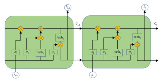
Figure 4.
LSTM basic schematic.
The cell state is the key to the LSTM, and the role of the gate is to add or remove information to the cell state. Among them, σ represents the sigmoid network layer. is the forget gate, the sigmoid layer outputs 0 to indicate discard, and output 1 to indicate complete retention. is called the input gate; it decides which states in the cell to update, and the layer decides the size of the updated value. is called the output gate, the layer normalizes the cell state information, and the multiplication of the two determines the LSTM output value. The following formula gives the description of the LSTM.
where represents the weight of input gate, output gate, and forget gate. represents bias terms. represents activation function. describes the vector element-wise product. represents cell state. represents intermediate value of .
4.2. LSTM Algorithm Aiding the SINS/DVL Navigation System
At present, the basic principle of using the LSTM model to assist the integrated navigation algorithm is mainly to train the LSTM model when the auxiliary sensor is normal; when the sensor fails, the deep learning model is used to provide an output that can correct the inertial navigation error. The commonly used AI model output is a three-dimensional velocity value similar to the DVL output, so we also choose this output mode [16,17,18,19].
As described in [20], to improve the accuracy and reliability of model predictions, AI models should choose valid inputs as training sets. Thus, we should explore the relationship of the variables in the integrated navigation system. Here we start from the inertial navigation update equation. The following is the selection of training input.
First, it is assumed that the velocity of SINS at time m is . At this time, if we want to obtain a relatively accurate DVL velocity measurement , attitude transformation is necessary. can be expressed as Formula (39):
In Formula (35), the meaning of each expression is as follows.
In Formula (41), can be described as Formula (42).
It can be seen from Formula (41) and (42), depends on the , , , , , and . The motion velocity of the underwater vehicle is relatively small, so the two quantities have little impact on . depends on the geographical location, the magnitude change can also be ignored. includes the , , . Compared with land carriers, such as automobiles, the three angles of underwater vehicles must be taken into account. Therefore, we get several quantities that have a large impact on the .
The schematic diagram of the specific deep learning model-assisted combined navigation is as Figure 5:
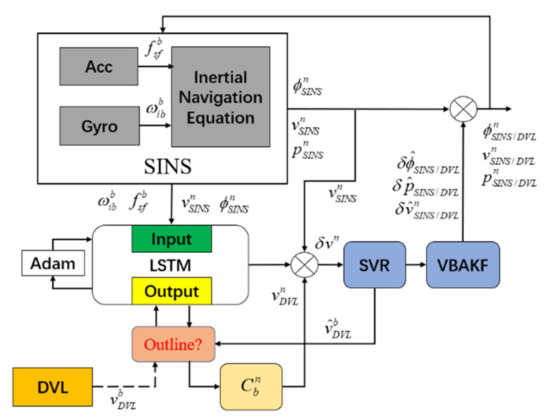
Figure 5.
Schematic diagram of deep learning model-assisted navigation system.
5. Test Results
First, the experimental scene and test equipment need to be described. This test uses a set of shipborne data with a duration of approximately 9000 s, and the test ship is equipped with IMU and DVL. At the same time, it is equipped with a single-antenna GPS receiver, which outputs position information at a frequency of 1 Hz. The main performance indicators of the relevant test equipment are shown in the Table 1 and Table 2.

Table 1.
The performance of IMU.
Table 2.
The performance of DVL.
5.1. Performance Experiment of Information Fusion Method
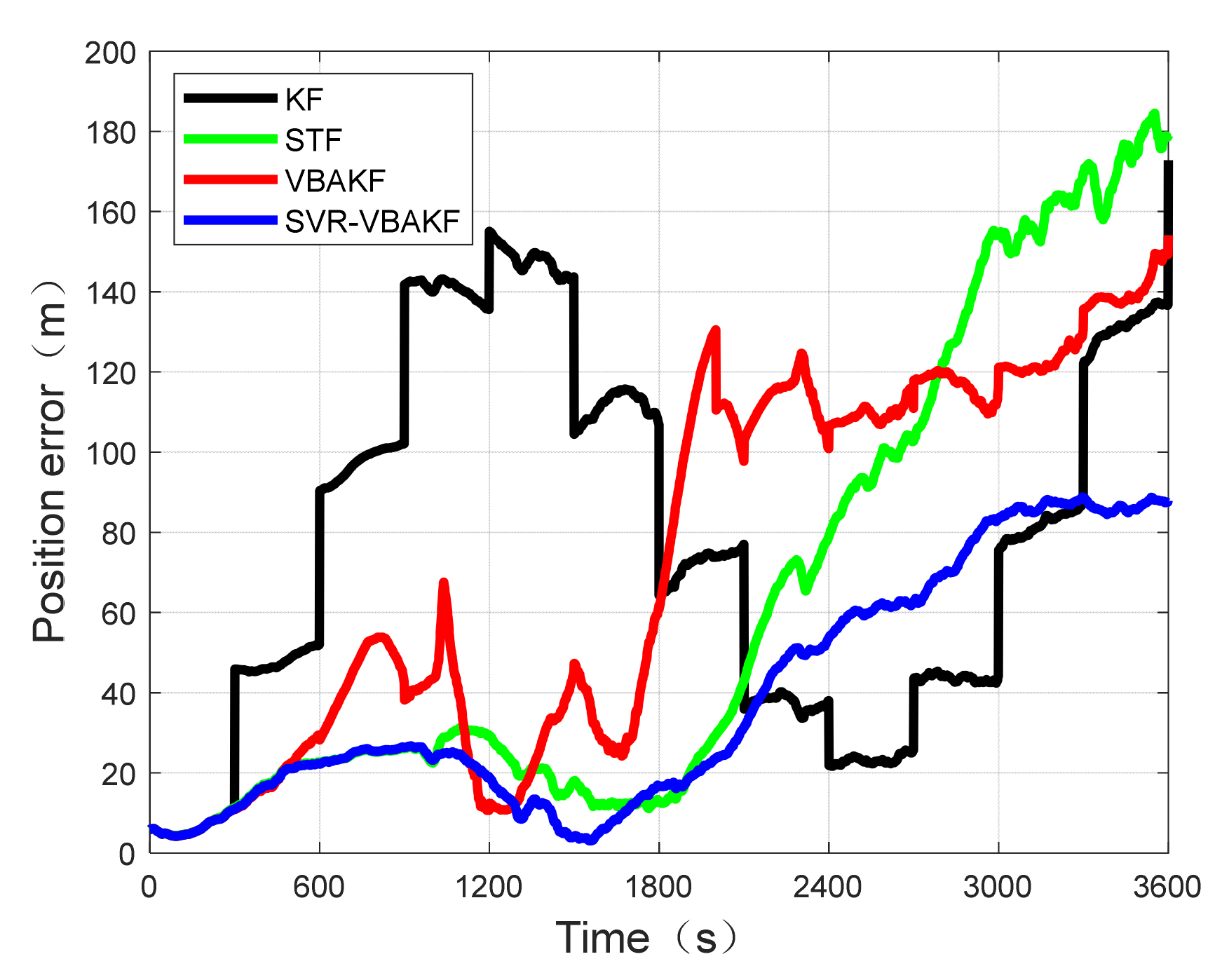
The evaluation of information fusion methods mainly includes the following methods, which are compared: the traditional Kalman filtering algorithm (KF), strong tracking Kalman filtering algorithm (STF), variational Bayesian adaptive filtering algorithm. The VBAKF algorithm) and the Support Vector Regression Aided Variational Bayesian Adaptive algorithm (SVR-VBAKF) result in integrated navigation tests. Among them, for the strong tracking filtering method, we adopt the novel robust filtering algorithm proposed in [42]. Here, the first 3600 s of data of the entire data segment is selected for the experiment of integrated navigation. It is undeniable that the system is very susceptible to the interference of the environment, especially during the on-board test and the outliers are easy to occur during the measurement process. Therefore, to evaluate the proposed algorithm, outliers were added every 300 s during the entire data segment. Here, the outliers are the same as the outliers of the original measurement data.
The initialization parameters of the navigation parameters are selected as the result of SINS/GPS integrated navigation since the support vector regression auxiliary filtering algorithm requires the interval processing of data. The length of the sliding window and the model order should be determined, here we select N = 20, m = 5, the fading factor ρ = 0.98, and the tuning parameter τ = 4 in the new method. In order to evaluate the effect of navigation, this paper uses position, velocity, and yaw error as the evaluation indicators of the filtering method. The error curves of the four filtering methods are in Figure 6, Figure 7 and Figure 8.

Figure 6.
Comparison of position errors.

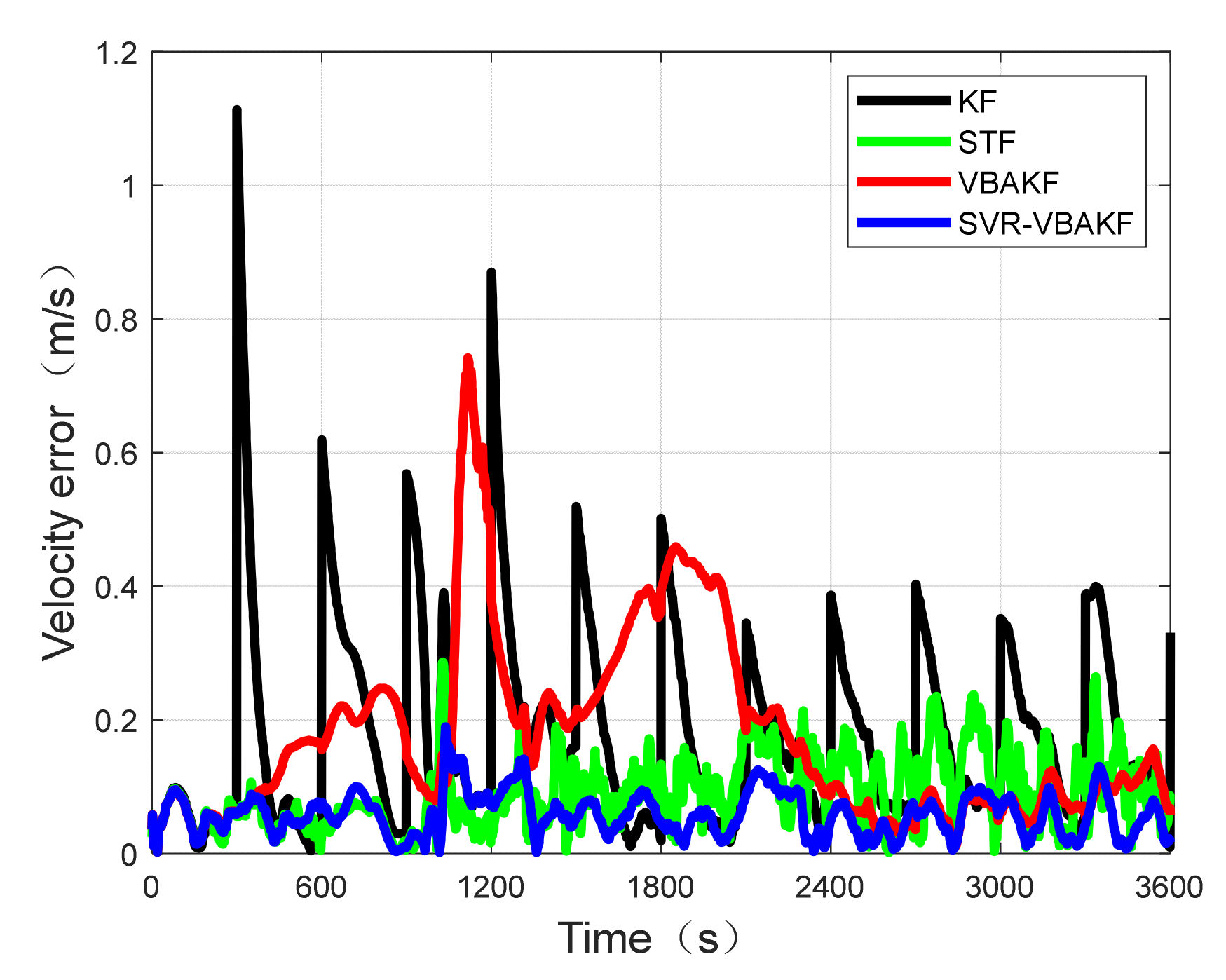
Figure 7.
Comparison of velocity errors.
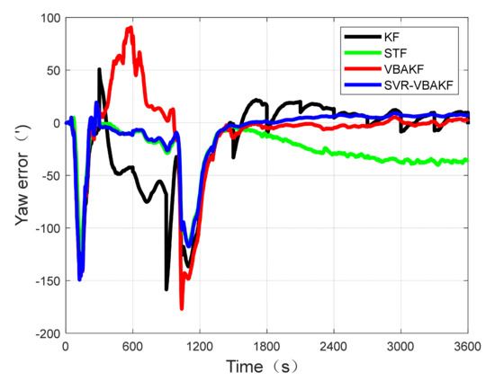
Figure 8.
Comparison of Yaw errors.
From the above pictures, we can see that the SINS/DVL integrated navigation result is divergent in the position error. Because the velocity is used as the intermediate quantity of information fusion, the effect of velocity error suppression is obvious, and the effect on the position and heading direction is not obvious. When there is no outlier interference, the combined navigation results of the three methods tend to be stable. However, when the DVL output is influenced by outliers, the traditional KF method is getting worse. Compared with the VBAKF method, it shows a good effect of resisting outliers in a certain period of time. As time grows, its robustness will deteriorate, resulting in unsatisfactory results, but better than the KF method. The robustness of the STF filtering method to the velocity error is obvious, and when the filtering time is approximately 2000 s, the effect of the position error and heading error is no less than the filtering algorithm newly proposed, but with the passage of time, the position error diverges quickly, and the heading error increases significantly. The VBAKF method assisted by SVR has obvious robustness to outliers and self-adaptation to noise, the position error has an obvious decreasing trend, the velocity error suppression effect is obvious, and the heading and attitude estimation has a faster convergence speed and a higher accuracy. The above table shows the mean square error (RMSE) of the combined navigation position, velocity, and heading of the three methods.
From the Table 3, the position error of the SVR-VBAKF method is increased by 47.63% compared with the KF method, which is 43.35% higher than that of the STF method. which is 39.82% higher than the VBAKF method. As for the KF method, the velocity error is improved by 67.25%, compared with 26.16% by the STF method, and improved by 60.13% compared with the VBAKF method. Compared with the KF method, the heading error is reduced by 29.61%, 43.35% higher than the STF method, 13.98% higher than the STF method, and 20.72% higher than the VBAKF method.
Table 3.
Root mean square errors of position, velocity, yaw.
5.2. Experiment of LSTM Model Aided Navigation System
The flow of the LSTM-assisted navigation system is shown in the last section. The LSTM module and the information fusion method are relatively independent, but when the SVR algorithm detects that the DVL measurement value is an outlier, the LSTM output is used to replace the outlier at this time. The system adopts the way of close loop mode. When the DVL normally provides measurement values, the LSTM training process, iterative optimization method, and filtering module continue to maintain high-precision navigation results.
The whole test lasted for 9000 s. Firstly, we use the first 70% of the whole data as the input of the LSTM model. The next 30% of the data is used to test the accuracy of the results output by the LSTM model. It is also to simulate the situation that the DVL output is interrupted, and use the attitude, velocity, specific force, and angular velocity to obtain credible “pseudo-measurement values”. The obtained “pseudo-measurement values” is to ensure the continuous progress of the information fusion method, and to use the SINS/DVL integrated navigation to suppress the trend of navigation error divergence caused by pure inertial navigation. The specific trajectory division is shown in the following figure: the green represents the training set, and test sets are indicated in red.
The LSTM module is selected as a regularized directional dropout layer and a fully connected layer (FC). The activation function of the fully connected layer is selected as the LeakyReLU. The output value of the activation function is used as the final output value of LSTM. The mean square error is used as the loss function. The number of neurons in the middle layer is set to be 128, and the training step is 4. The initial learning rate is 0.002, the decay factor is 5 × 10⁻⁴, the L1 regulation is 0.95, the L2 regulation is set to 0.99, and the number of training iterations are set to 300. Several deep learning models selected for the convenience of comparison have only one hidden layer, and the number of neurons in the hidden layer is 128. All the training samples should be normalized between −1 and 1 for accelerating the process of training. The input samples of LSTM-1, MLP, and NARX are in the form of neural network in the literature [18], and NARX is also the deep learning model selected in this literature. Just to compare with the model selected in this paper. LSTM-1 has the same structure as LSTM-2, and the input mode of the latter has been explained in Section 4. The specific training set and test set trajectory division are shown in Figure 9.
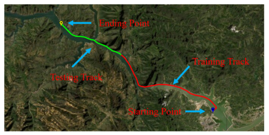
Figure 9.
Division diagram of training track and test track.
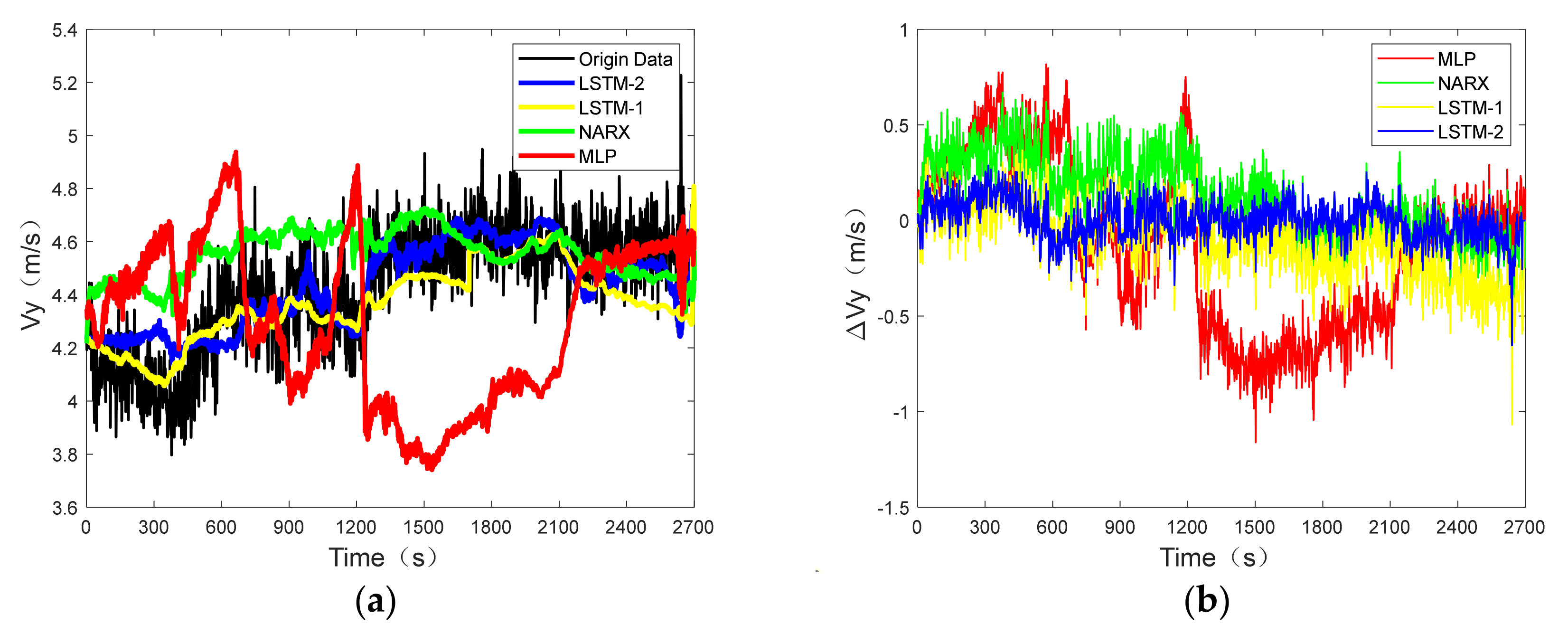
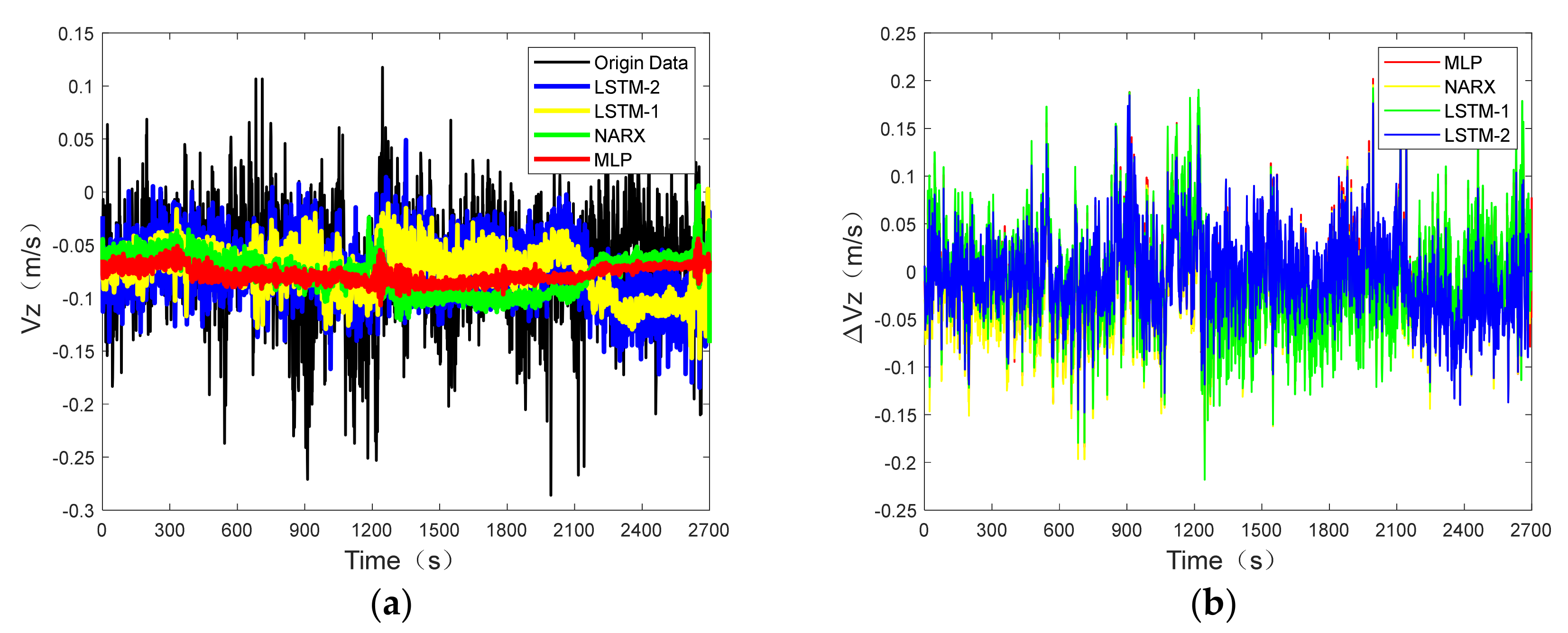
After offline training with different types and input modes of neural networks, modules that autonomously output “pseudo-measurement values” can be obtained. For comparison, the following Figure 10, Figure 11 and Figure 12 show the actual output and predicted output of different modules. Figure 13 shows the mean and STD of the predicted error.
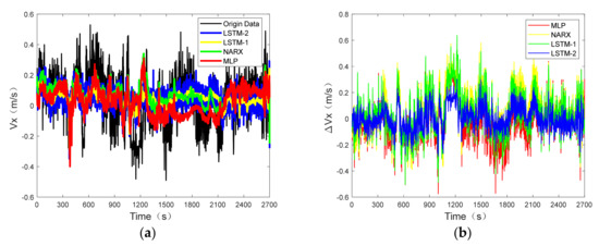
Figure 10.
Prediction results of east velocity: (a) Comparison of actual value and the predicted velocity in the east; (b) The errors of actual value and the predicted velocity in the east for different algorithms.

Figure 11.
Prediction results of north velocity: (a) Comparison of actual value and the predicted velocity in the north; (b) The errors of actual value and the predicted velocity in the north for different algorithms.

Figure 12.
Prediction results of vertical velocity: (a) Comparison actual value and the predicted velocity in the vertical; (b) The errors of actual value and the predicted velocity in the vertical for different algorithms.

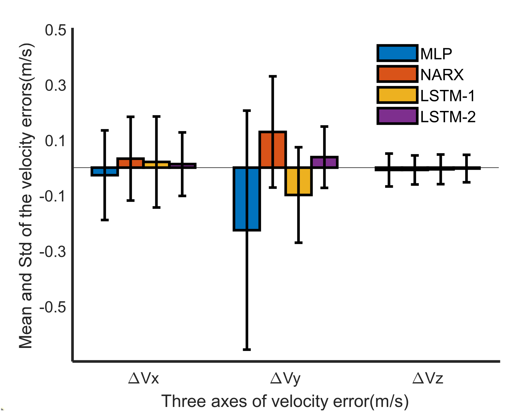
Figure 13.
Error MEAN and STD of four deep learning models.
As can be seen from the above three figures and Table 4, the average velocity error of the LSTM-2 model in the three directions is reduced by 55.43%, 57.30%, and 83.40%, compared with the MLP network. Compared with the NARX model, it is reduced by 61.68%, 70.82%, and 54.76%. Compared with the LSTM-1 model, it is reduced by 39.40%, 62.04%, and 57.30%. In addition, for the velocity errors standard deviation compared with the MLP network, they are reduced by 35.23%, 74.30%, and 32.94%. Compared with the NARX model, they are reduced by 30.78%, 44.79%, and 35.73%. Compared with the LSTM-1 model, they are reduced by 36.21%, 35.73%, and 32.94%.
Table 4.
The specific values of the error MEAN and STD of the four deep learning models.
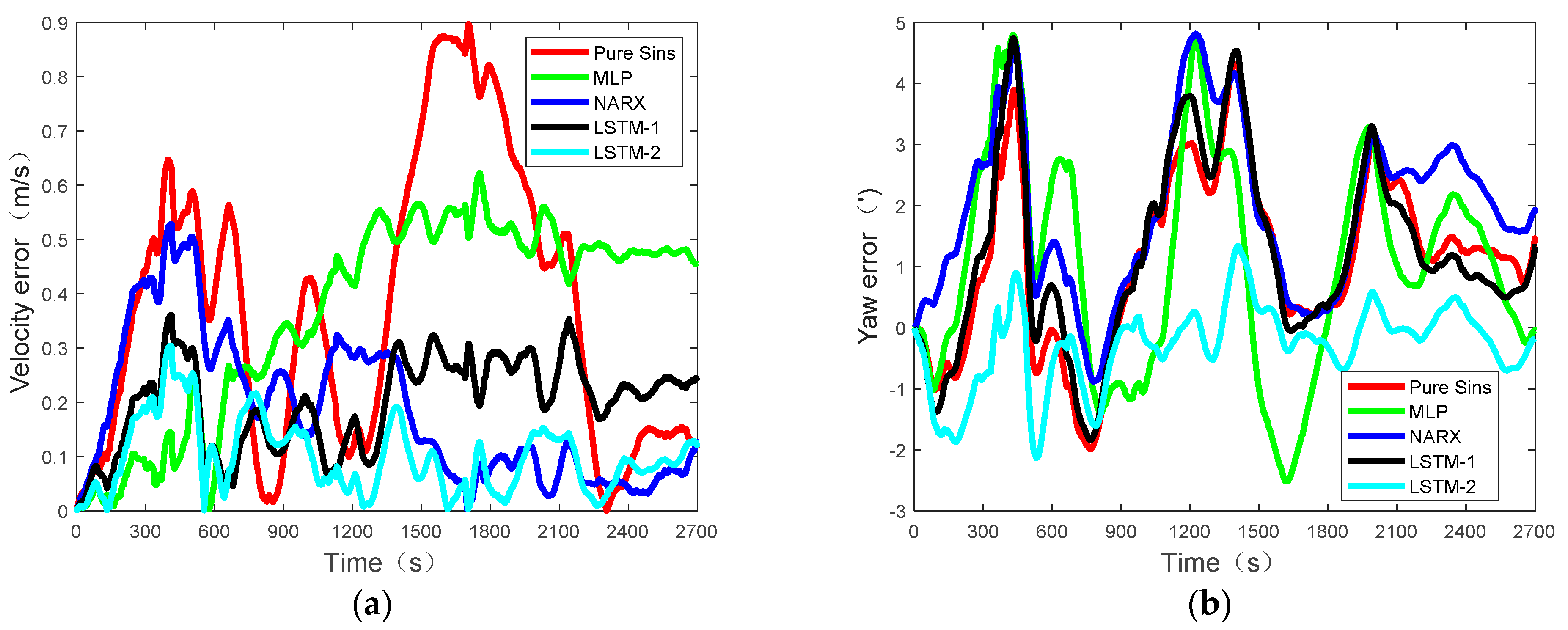
If we only use the fitting effect to illustrate the combined navigation results, it is not enough. It is necessary to use “pseudo measurements” for continuous navigation. The information fusion method used in the integrated navigation here refers to the SVR-VBAKF method described in the previous section. Therefore, the four deep learning models use this method. As an important index to evaluate the effect of integrated navigation, the position error, velocity error, and heading error are also introduced here for evaluation. The specific integrated navigation errors are in the following, Figure 14 and Figure 15.
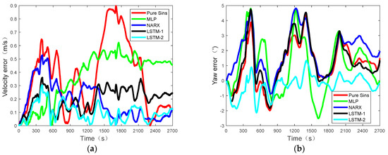
Figure 14.
Comparison of navigation velocity and yaw error results: (a) Comparison of velocity errors.; (b) Comparison of yaw errors.
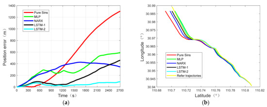
Figure 15.
Comparison of navigation position error results: (a) Comparison of position errors; (b) Trajectory diagram in the case of DVL failure.
From Table 5 and Figure 14 and Figure 15, we can obtain the position error, velocity error, and heading error results of using different deep learning models to assist SINS/DVL combined navigation. The LSTM-based hybrid prediction method we adopted here is optimal compared to other deep learning models, both in terms of measurement value prediction and combination navigation using “pseudo-measurement values”. This is why we do not choose the navigation errors as the training simples. Compared with the navigation information output by the SINS selected in this paper, the incremental form is not closely related, so the result of combined navigation is poor. However, as an input sample in the incremental form, LSTM is obviously stronger for two deep learning models, MLP and NARX. In the 2700 s DVL environment, the position error predicted by the LSTM-2 method is reduced by 85.93%, 83.94%, and 75.64%, and the velocity error is reduced by 73.69%, 47.66%, and 44.53%, respectively, compared with the other three methods. Except for the proposed method, the heading error is not well suppressed, but the errors are all within 1. Compared with the pure inertial solution, the heading error of the LSTM-2 method is reduced by 57.17%. The above experiments show that the proposed hybrid prediction method can effectively suppress the SINS error in the environment of short-term DVL failure, and effectively improve positioning accuracy.
Table 5.
Integrated navigation position, velocity, heading error table.
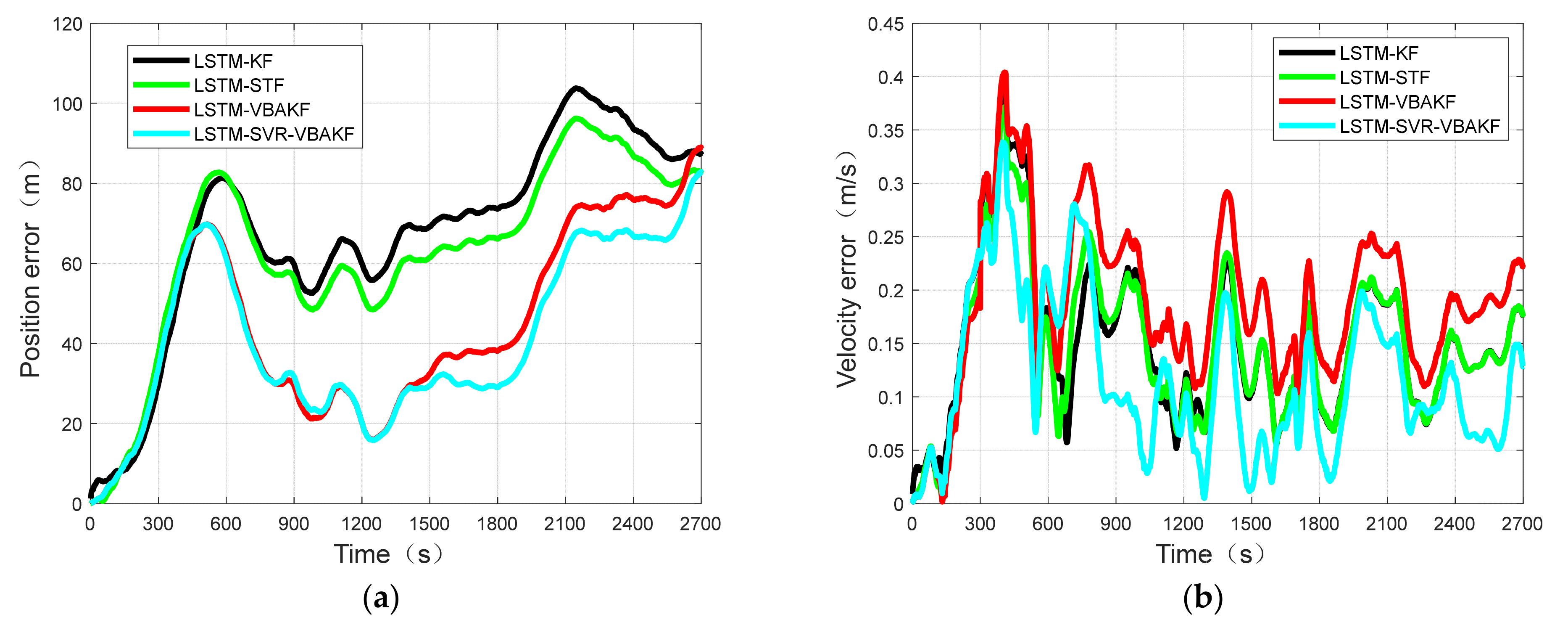
Integrated navigation errors of different deep learning models under the same information fusion method have been discussed in Figure 16. In order to fully illustrate the advantages of the method, a comparison of filtering methods under the same deep learning model is carried out. The deep learning model here adopts the deep learning model of LSTM-2 and uses different filtering methods for error comparison. Here, for the convenience of research, we only introduce position error and velocity error for evaluation.
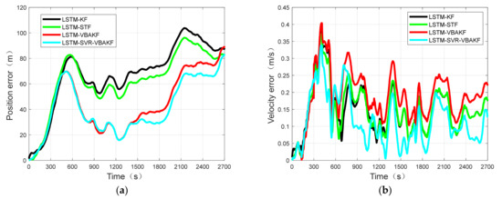
Figure 16.
Comparison of navigation position and velocity error results: (a) Comparison of position errors; (b) Comparison of velocity errors.
In Figure 16, the curves of velocity and position error that the SVR-VBAKF filter under the same deep learning model can show better navigation performance than other methods.
6. Conclusions
Aiming at the problem of velocity failure of DVL, we propose a new solution process, which effectively reduces outlier interference in the integrated navigation process and improves the accuracy of the system. At the same time, the filter based on VB can also enhance adaptability to the environment. When the output of DVL is interrupted within a certain time, the LSTM deep learning method is used to provide the “pseudo-measurement value,” which is used for integrated navigation. This method collects the original information of the SINS as a sample in the normal working mode of the DVL, trains the LSTM, using the well-trained LSTM model to assist the output when the DVL fails. The LSTM/SVR-VBAKF algorithm effectively improves the processing ability of the integrated navigation system to output faults and the suppression of navigation errors. The on-board experiment proves the superiority and effectiveness of the proposed method.
Author Contributions
Resources, J.Z. and J.W.; software, J.Z. and F.Q.; writing—original draft, J.Z.; writing—review and editing, J.Z. H.C., F.Q. and A.L. All authors have read and agreed to the published version of the manuscript.
Funding
This research was funded by the National Natural Science Foundation of China under grant 61873275; this research was also funded by the Natural Science Foundation of Hubei Province of China (2017CFB377).
Institutional Review Board Statement
Not applicable.
Informed Consent Statement
Not applicable.
Data Availability Statement
No new data were created or analyzed in this study. Data sharing is not applicable to this article.
Conflicts of Interest
The authors declare no conflict of interest.
References
- Fukuda, G.; Hatta, D.; Guo, X.; Kubo, N. Performance evaluation of IMU and DVL integration in marine navigation. Sensors 2021, 21, 1056. [Google Scholar] [CrossRef] [PubMed]
- Stutters, L.; Liu, H.C. Navigation technologies for autonomous underwater vehicles. IEEE Trans. Syst. Man Cybern. C Appl. Rev. 2008, 38, 581–589. [Google Scholar] [CrossRef]
- Huang, S.W.; Taniguchi, N.; Huang, C.F.; Guo, J. Autonomous underwater vehicle navigation using a single tomographic node. J. Acoust. Soc. Am. 2016, 140, 3075–3090. [Google Scholar] [CrossRef]
- Li, Z.; Wang, Y.; Yang, W.; Ji, Y. Development status and key navigation technology analysis of autonomous underwater vehicles. In Proceedings of the 2020 3rd International Conference on Unmanned Systems (ICUS), Harbin, China, 27–28 November 2020; pp. 1130–1133. [Google Scholar]
- Affleck, C.; Jircitano, A. Passive gravity gradiometer navigation system. In Proceedings of the IEEE Symposium on Position Location and Navigation. A Decade of Excellence in the Navigation Sciences, Las Vegas, NV, USA, 20 March 1990; pp. 60–66. [Google Scholar]
- Troni, G.; Whitcomb, L.L. Advances in in situ alignment calibration of Doppler and high/low-end attitude sensors for underwater vehicle navigation: Theory and experimental evaluation. J. Field Robot. 2015, 32, 655–674. [Google Scholar] [CrossRef]
- Morgado, M.; Batista, P.; Oliveira, P.; Silvestre, C. Position USBL/DVL sensor-based navigation filter in the presence of unknown ocean currents. Automatica 2011, 47, 2604–2614. [Google Scholar] [CrossRef]
- Yan, Z.; Wang, L.; Wang, T.; Yang, Z.; Chen, T.; Xu, J. Polar cooperative navigation algorithm for multi-unmanned underwater vehicles considering communication delays. Sensors 2018, 18, 44. [Google Scholar] [CrossRef]
- Liu, P.; Wang, B.; Deng, Z.H.; Fu, M.Y. INS/DVL/PS tightly coupled underwater navigation method with limited DVL measurements. IEEE Sens. J. 2018, 18, 2994–3002. [Google Scholar] [CrossRef]
- Zhang, L.; Wu, W.Q.; Wang, M.S.; Guo, Y. DVL-aided SINS in-motion alignment filter based on a novel nonlinear attitude error model. IEEE Access 2019, 7, 62457–62464. [Google Scholar] [CrossRef]
- Hegrenaes, Ø.; Hallingstad, O. Model-aided INS with sea current estimation for robust underwater navigation. IEEE J. Ocean. Eng. 2011, 36, 316–337. [Google Scholar] [CrossRef]
- Mirabadi, A. Fault detection and isolation in multisensor train navigation systems. In Proceedings of the KACC International Conference on Control (CONTROL ’98), Swansea, UK, 1–4 September 1998; pp. 969–974. [Google Scholar]
- Karmozdi, A.; Hashemi, M.; Salarieh, H.; Alasty, A. Implementation of Translational Motion Dynamics for INS Data Fusion in DVL Outage in Underwater Navigation. IEEE Sens. J. 2021, 5, 6652–6659. [Google Scholar] [CrossRef]
- Tal, A.; Klein, I.; Katz, R. Inertial Navigation System/Doppler Velocity Log (INS/DVL) Fusion with Partial DVL Measurements. Sensors 2017, 17, 415. [Google Scholar] [CrossRef] [PubMed]
- Wang, J.J.; Wang, J.; Sinclair, D.; Watts, L. A neural network and Kalman filter hybrid approach for GPS/INS integration. In Proceedings of the Korean Institute of Navigation and Port Research Conference; Korean Institute of Navigation and Port Research, 2006; pp. 277–282. Available online: https://koreascience.kr/publisher/kin.page (accessed on 9 September 2022).
- Wang, D.; Xu, X.; Yao, Y.Q.; Zhang, T. Virtual DVL reconstruction method for an integrated navigation system based on DS-LSSVM algorithm. IEEE Trans. Instrum. Meas. 2021, 70, 8501913. [Google Scholar] [CrossRef]
- Li, W.L.; Chen, M.; Zhang, C.; Zhang, L.; Chen, R. A novel neural network-based SINS/DVL integrated navigation approach to deal with DVL malfunction for underwater vehicles. Math. Problems Eng. 2020, 2020, 2891572. [Google Scholar] [CrossRef]
- Li, D.; Xu, J.N.; He, H.Y.; Wu, M. An Underwater Integrated Navigation Algorithm to Deal with DVL Malfunctions Based on Deep Learning. IEEE Access 2021, 9, 82010–82020. [Google Scholar] [CrossRef]
- Ansari-Rad, S.; Hashemi, M.; Salarieh, H. Pseudo DVL reconstruction by an evolutionary TS-fuzzy algorithm for ocean vehicles. Measurement 2019, 147, 106831. [Google Scholar] [CrossRef]
- Yao, Y.; Xu, X.; Li, Y.; Zhang, T. A hybrid IMM based INS/DVL integration solution for underwater vehicles. IEEE Trans. Veh. Technol. 2019, 68, 5459–5470. [Google Scholar] [CrossRef]
- Wang, D.; Xu, X.S.; Hou, L.H. An Improved Adaptive Kalman Filter for Underwater SINS/ DVL System. Math. Probl. Eng. 2020, 2020, 5456961. [Google Scholar] [CrossRef]
- Xu, B.; Guo, Y.C.; Hu, J. An Improved Robust Kalman Filter for SINS/DVL Tightly Integrated Navigation System. IEEE Trans. Instrum. Meas. 2021, 70, 8502915. [Google Scholar] [CrossRef]
- Liu, S.; Zhang, T.; Zhang, J.; Zhu, Y. A New Coupled Method of SINS/DVL Integrated Navigation Based on Improved Dual Adaptive Factors. IEEE Trans. Instrum. Meas. 2021, 70, 8504211. [Google Scholar] [CrossRef]
- Wang, Y.; Zheng, W.; Sun, S.; Li, L. Robust information filter based on maximum correntropy criterion. J. Guid. Control. Dyn. 2016, 39, 1126–1131. [Google Scholar] [CrossRef]
- Wang, G.; Zhang, Y.; Wang, X. Maximum correntropy Rauch-Tung Striebel smoother for nonlinear and non-Gaussian systems. IEEE Trans. Autom. Control 2021, 66, 1270–1277. [Google Scholar] [CrossRef]
- Chang, G.B. ‘Robust Kalman filtering based on mahalanobis distance as outlier judging criterion. J. Geodesy 2014, 88, 391–401. [Google Scholar] [CrossRef]
- Zhu, Y.; Cheng, X.; Hu, J.; Zhou, L.; Fu, J. A novel hybrid approach to deal with DVL malfunctions for underwater integrated navigation systems. Appl. Sci. 2017, 7, 759. [Google Scholar] [CrossRef]
- Qasem, S.N.; Ahmadian, A.; Mohammadzadeh, A.; Rathinasamy, S.; Pahlevanzadeh, B. A type-3 logic fuzzy system: Optimized by a correntropy based Kalman filter with adaptive fuzzy kernel size. Inf. Sci. 2021, 572, 424–443. [Google Scholar] [CrossRef]
- Chang, L.B.; Qin, F.J.; Wu, M.P. Gravity disturbance compensation for inertial navigation system. IEEE Trans. Instrum. Meas. 2019, 68, 3751–3765. [Google Scholar] [CrossRef]
- Gao, D.Y.; Hu, B.Q.; Qin, F.J.; Chang, L.B. A Real-Time Gravity Compensation Method for INS Based on BPNN. IEEE Sens. J. 2021, 21, 13584–13593. [Google Scholar] [CrossRef]
- Li, W.L.; Wu, W.Q.; Wang, J.; Lu, L. A fast SINS initial alignment scheme for underwater vehicle applications. J. Navigat. 2013, 66, 181–198. [Google Scholar] [CrossRef]
- Zhu, B.; He, H.Y. Integrated navigation for Doppler velocity log aided strapdown inertial navigation system based on robust IMM algorithm. Optik 2020, 217, 164871. [Google Scholar] [CrossRef]
- Chang, L.B.; Li, Y.; Xue, B. Initial alignment for a Doppler velocity log-aided strapdown inertial navigation system with limited information. IEEE/ASME Trans. Mechatron. 2017, 22, 329–338. [Google Scholar] [CrossRef]
- Wang, B.; Liu, H.; Liu, J.Y.; Deng, Z.H.; Fu, M.Y. A Support Vector Regression Based Integrated Navigation Method for Underwater Vehicles. IEEE Sens. J. 2020, 20, 8875–8883. [Google Scholar] [CrossRef]
- Zhou, P.; Guo, D.; Wang, H.F.; Chai, T. Data-Driven Robust M-LS-SVR Based NARX Modeling for Estimation and Control of Molten Iron Quality Indices in Blast Furnace Ironmaking. IEEE Trans. Neural Netw. Learn. Syst. 2018, 29, 4007–4021. [Google Scholar] [CrossRef] [PubMed]
- Ren, Y.; Suganthan, P.N.; Srikanth, N. A Novel Empirical Mode Decomposition WITH Support Vector Regression for Wind Speed Forecasting. IEEE Trans. Neural Netw. Learn. Syst. 2016, 27, 1793–1798. [Google Scholar] [CrossRef] [PubMed]
- Yu, M.-J. INS/GPS integration system using adaptive filter for estimating measurement noise variance. IEEE Trans. Aerosp. Electron. Syst. 2012, 48, 1786–1792. [Google Scholar] [CrossRef]
- Huang, Y.L.; Zhang, Y.G.; Wu, Z.M.; Li, N.; Chambers, J. A Novel Adaptive Kalman Filter with Inaccurate Process and Measurement Noise Covariance Matrices. IEEE Trans. Autom. Control. 2018, 63, 594–601. [Google Scholar] [CrossRef]
- Fang, W. A LSTM algorithm estimating pseudo measurements for aiding INS during GNSS signal outages. Remote Sens. 2020, 12, 256. [Google Scholar] [CrossRef]
- Liu, J.; Guo, G. Vehicle localization during GPS outages with Extended Kalman Filter and Deep Learning. IEEE Trans. Instrum. Meas. 2021, 70, 7503410. [Google Scholar] [CrossRef]
- Wagstaff, B.; Kelly, J. LSTM-based zero-velocity detection for robust inertial navigation. In Proceedings of the 2018 International Conference on Indoor Positioning and Indoor Navigation (IPIN), Nantes, France, 24–27 September 2020; IEEE: Piscataway, NJ, USA, 2020; pp. 1–8. [Google Scholar]
- Xiong, H.L.; Tang, J.; Xu, H.J.; Zhang, W.S.; Du, Z.F. A Robust Single GPS Navigation and Positioning Algorithm Based on Strong Tracking Filtering. IEEE Sens. J. 2018, 18, 290–298. [Google Scholar] [CrossRef]


Publisher’s Note: MDPI stays neutral with regard to jurisdictional claims in published maps and institutional affiliations. |
© 2022 by the authors. Licensee MDPI, Basel, Switzerland. This article is an open access article distributed under the terms and conditions of the Creative Commons Attribution (CC BY) license (https://creativecommons.org/licenses/by/4.0/).