Abstract
Air pollution has become a global issue due to its widespread impact on the environment, economy, civilization and human health. Owing to this, a lot of research and studies have been done to tackle this issue. However, most of the existing methodologies have several issues such as high cost, low deployment, maintenance capabilities and uni-or bi-variate concentration of air pollutants. In this paper, a hybrid CNN-LSTM model is presented to forecast multivariate air pollutant concentration for the Internet of Things (IoT) enabled smart city design. The amalgamation of CNN-LSTM acts as an encoder-decoder which improves the overall accuracy and precision. The performance of the proposed CNN-LSTM is compared with conventional and hybrid machine learning (ML) models on the basis of Mean Absolute Error (MAE), Mean Absolute Percentage Error (MAPE) and Mean Square Error (MSE). The proposed model outperforms various state-of-the-art ML models by generating an average MAE, MAPE and MSE of 54.80%, 52.78% and 60.02%. Furthermore, the predicted results are cross-validated with the actual concentration of air pollutants and the proposed model achieves a high degree of prediction accuracy to real-time air pollutants concentration. Moreover, a cross-grid cooperative scheme is proposed to tackle the IoT monitoring station malfunction scenario and make the pollutant monitoring more fault resistant and robust. The proposed scheme exploits the correlation between neighbouring monitoring stations and air pollutant concentration. The model generates an average MAPE and MSE of 10.90% and 12.02%, respectively.
1. Introduction
In the last two decades, the air quality has become progressively worse due to rapid industrialization and urbanization. Most of these air pollutants eventuate in the ambient due to various reasons such as automobile emission, industrial emission, fossil fuel burning and wastage incarceration. These air pollutants penetrate the human body and cause various chronic respiratory and heart-related diseases. According to the World Health Organization (WHO), more than 90% of the world population lives in perilous air quality areas. Each year nearly 4.2 million deaths occur from cardio and respiratory diseases due to prolonged exposure to air pollutants [1]. According to another report by WHO, each year, around 3.8 million die due to diseases attributed to indoor house pollution [2]. Furthermore, air pollution is one of the root causes of climate change and restricts the social as well as economic development of the country [3].
To address this issue, national environmental agencies monitor and track carbon monoxide (), fine particulate matter (), respirable particulate matter (), sulfur dioxide (), nitrogen dioxide () and ozone () in the environment to determine air quality, often called as Air Quality Index (AQI). The , , and are measured in part-per-million (ppm) while and is measured in micrograms per meter cube (μg/m3). It is a standard metric to evaluate the quality of air, whether it is hazardous, unhealthy, moderate or good (as shown in Table 1). Many governments and environmentalists use these standard values to identify whether the air quality is good or bad and poses a little or high risk to the population. The AQI can help citizens to take precautionary measures in a timely manner.

Table 1.
Summary of air pollutant standards and classification.
Recently, researchers and scientists have proposed multiple solutions to monitor and mitigate the impact of air pollution on both the ambient and humans. Several data-centric and geological time scale-based studies have been done to provide extensive insights and issues pertaining to air quality [4,5]. Moreover, various innovative ideas, such as the integration of artificial intelligence (AI) and machine learning (ML), have been presented for better accuracy and prediction. A neural network (NN) based framework has been proposed to forecast for Seoul subway station [6]. A hybrid long short-term memory (LSTM) base model is presented to improve the prediction accuracy of [7]. Multi-model architectures have been presented to monitor and predict and for urban areas [8,9].
However, with the development of the Internet of Things (IoT), a new paradigm has emerged that transformed the traditional human lifestyle into a high-tech lifestyle. Nowadays, IoT devices assist humans in performing daily tasks due to their ease of deployment, low cost and very low maintenance nature. Researchers have proposed multiple IoT base ambient monitoring solutions employing Wireless Fidelity (WiFi), Zigbee, Bluetooth and LoRaWAN [10,11,12,13]. These IoT devices are distributed over the region for ambient monitoring. These devices gather ambient air pollution data and forward it to the base station for information processing and distribution among citizens (as shown in Figure 1). Furthermore, integrating IoT devices with AI & ML techniques can enable them to incorporate the acquired data to predict the next hour or day’s AQI.
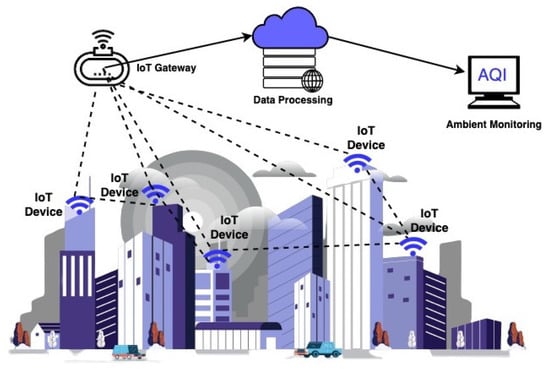
Figure 1.
Internet of Things base ambient pollution monitoring and forecasting system architecture.
The motivation of this study is to develop a lightweight multivariate ambient monitoring system that is self-reliant and independent in terms of accuracy and processing. The main contribution of this paper is as follows:
- 1.
- A two-layer prediction model; CNN and LSTM, has been presented for air pollutants concentration forecasting. The proposed model is utilised to predict the concentration of air pollutants by the hour for 7 days. Furthermore, the prediction results are cross-validated with real-time data.
- 2.
- In this paper, multivariate elements (, , , , and ) are taken into account. However, most of the previous research takes either one or two air pollutant elements into consideration.
- 3.
- The performance of the proposed CNN-LSTM model is compared with the various state-of-the-art frameworks on the basis of Mean Absolute Error, Mean Absolute Percentage Error and Mean Square Error.
- 4.
- IoT devices are prone to failure, crash or malfunction. A weight-fused cooperative approach is proposed by integrating cross-grid neighbouring monitoring stations with temporal malfunction monitoring station data to tackle this issue.
- 5.
- A comprehensive study and analysis are performed on 24 months of real-world time series data to evaluate the performance of the proposed scheme.
The rest of the paper is organised as follows. Section 2 discusses the state-of-the-art work related to ambient monitoring and prediction. In Section 3, the implementation of the system, dataset and its preprocessing are discussed in detail. Section 4 presents the proposed approach for normal as well as malfunctioned monitoring station scenarios. Results and discussion are presented in Section 5. Finally, Section 6 presents an overall conclusion of the proposed approaches with future direction.
2. Related Work
In recent years, a lot of significant contributions have been made in the area of IoT base ambient monitoring systems. In this section, we present the state-of-the-art research frameworks that have been proposed in this area.
In 2008, China initiated a joint control task force to control and tackle air pollution in Beijing, Hebei and Tianjin Province [14]. This controlled ambient air quality produces some good results and experiences for residents. In Ref. [15], the authors proposed a wireless sensor network (WSN) based intelligent ambient temperature monitoring scheme called a solar radiation-based air temperature error correction scheme (STCS). The proposed scheme used Back Propagation integrated with a Genetic algorithm for performance optimization. The authors of [16] proposed an RF-CNN-based AQI classification model. The proposed model uses ambient images for training and testing and classifies the AQI of the monitoring area as good, moderate and bad. In Ref. [17], an LSTM and Recurrent Neural Network (RNN) based prediction model has been proposed for IoT-enabled areas to forecast . The proposed model achieves higher accuracy in forecasting in comparison with LSTM.
In Ref. [18], the authors proposed an intelligent monitoring system for the indoor environment using WSN. The objective of this research is to provide a real-time ambient monitoring system with minimal interferences and error rates. In Ref. [19], a fully connected LSTM (LSTM-FC) base model is proposed to monitor and predict by exploiting temporal weather and air quality data. The proposed model performs better in comparison with the LSTM and Artificial Neural Network (ANN) in terms of Root Mean Squared Error (RMSE) and Mean Absolute Error (MAE).
The authors of [20] discussed the strengths and weaknesses of statistical and ML base methods for intelligent ambient monitoring. They suggested that the integration of ML with the temporal data to monitor and predict air quality is best suited. In Ref. [21], the authors proposed a deep learning-based ambient monitoring system to predict the concentration of air pollutants in the dataset of Seoul, South Korea. The proposed model outperforms other models with an MAE and MAPE of 11.43% and 1.64%, respectively. In Ref. [22], a comparative study of 36 ML models has been done to predict the indoor temperature for smart buildings. The ExtraTree regressor outperformed the other model with an RMSE of 0.058% and an accuracy of 97%, respectively. Authors of [23] proposed an IoT base real-time context-aware indoor ambient monitoring system. The proposed model uses Multiple linear regression (MLR) to calculate the concentration of , and . Furthermore, they integrate k-nearest neighbours (kNN) to forecast indoor ventilation and air pollutants. The proposed kNN-MLR was performed with an accuracy of 94% and a precision of 91%, respectively.
The authors of [24] presented a power-independent WSN-based ambient monitoring system for smart city design. The proposed system uses LoRaWAN to connect and communicate between sensors. However, it uses GPRS to forward the data to the cloud. In Ref. [25], a low-power WSN-based real-time ambient monitoring system has been proposed using LoRaWAN. The proposed system monitors and with 97% and 96% of accuracy respectively. Authors of [26] proposed an IoT base ambient monitoring system with minimal energy consumption and leakage. The proposed methodology is implemented in a laboratory-controlled environment. However, the authors fail to validate the results with in-field acquired data and the long-term stability of the IoT network. In Ref. [27], a hybrid ambient monitoring system is presented by integrating fixed as well as moving IoT sensors to calculate and predict the air pollutant with a primary focus on and . They opted for the Gradient Boosting Regression (GBR) technique for the prediction of air pollutants due to its adaptation to the change in the pattern. The proposed model performs better in terms of RMSE in comparison with the Random Forest (RF) and Support Vector Regression (SVR).
Evidently, most of the previous research lacks multivariate air pollutant monitoring and prediction. They only monitor either one or two air pollutant elements. Traditional ambient monitoring systems are complex, compute-intensive and require higher processing [7,8,9,23,25]. Furthermore, they are incapable of a scenario if an ambient monitoring station (MS) malfunctions, breakdown and power loss.
3. Dataset Preparation
In this section, the proposed methodology and implementation are discussed in detail. First, we will converse about monitoring stations and the dataset. Later on, the preprocessing of the dataset, which techniques have opted and how we clean and transform it are comprehensively discussed.
3.1. IoT Monitoring Stations
This research is carried out in Seoul, South Korea, which is envisioned as a smart city [28] and the biggest cosmopolitan city in the Republic of Korea. In 2021, Seoul ranked 26th among the most polluted cities in the world [29,30]. Henceforth, the Government of Korea deployed IoT-based MS all over the city (as shown in Figure 2) to tackle this issue. These MS are used to monitor ambient pollution continuously. The acquired data is made public through the official online data repository for researchers, scientists and the general public.
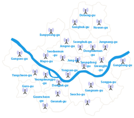
Figure 2.
Deployment of IoT monitoring stations in Seoul.
Seoul city is overall spatial segmented into 25 regions for ambient pollution monitoring using IoT-MS, which are uniformly dispersed all over the city. The longitude range of ambient MS is from 126.908296 to 127.068505, while the latitude range is from 37.452357 to 37.658774. The location of each MS is shown in Appendix A.
3.2. Dataset
In this study, we used a raw dataset acquired from an online data repository in Seoul, Republic of Korea [31]. The acquired dataset spanned from 1 January 2017 to 31 December 2019, in which measured the air pollutant concentration on an hourly basis. The overall dataset consists of almost 650,000 instances where each instance consists of Longitude, Latitude, Station Name, Station Code, Station Address, Measurement Date, Time and concentration of , , , , and .
The mathematical model of the dataset is formulated through a generic matrix (as shown in Equation (1)).
In Equation (1), represents the input from the MS, n represents the total number of MSs and t represents the time where . All of this information is integrated and an overall AQI of the city is determined.
Since the acquired dataset contains noise, missing values and outliers, hence we need to preprocess the data to develop a robust air pollution forecasting model.
3.3. Preprocessing of Data
The output of the forecasting model can be significantly impacted and reduced with the presence of noise, missing values, outliers, etc. in the dataset. Henceforth, to make the proposed model more robust, several preprocessing techniques are employed.
3.3.1. Anomalies Detection
The term “anomalies” refers to a small slice of the dataset which is abnormal or dissimilar to the rest of the data. It can be noisy data owing to random mistakes, or it can be irregular data items arising from odd or unexpected events that reflect aberrant behaviour. A rapid change in the values or values less than or equal to 0 is generally considered an anomaly in the dataset. These anomalies directly affect the learning of models as well as the model output. Henceforth, before forwarding the dataset to the model, outliers are identified along with the time series.
In this study, we only consider those air pollutants concentration values which are less than 0 as anomalies or outliers (as shown in Figure 3). During the close investigation of the dataset, it has been observed that the rapid change in air pollutant concentration occurred during public holidays due to festive celebrations, excessive vehicular emissions, etc. Subsequently, a total of 4992 anomalies/outliers are detected throughout the dataset. Most of these anomalies are due to the malfunctioning or failure of the monitoring station (). All these anomalies are removed to ensure consistency and uniformity in the dataset.
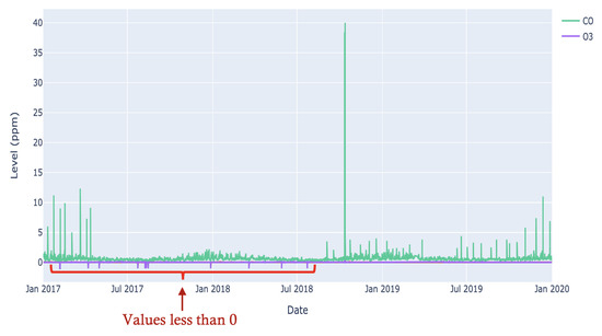
Figure 3.
Anomalies in the and dataset.
3.3.2. Data Normalization
Air pollutants are measured at different scales like , , and are calculated in parts per million (ppm) while and are calculated in microgram per cubic meter (μg/m3). Subsequently, the dataset is transformed between the range of 0 and 1 using Equation (2), to eliminate the dimensional difference impacts [32].
In Equation (2), represents the data after normalization while and represent the minimum and maximum values of each air pollutant value. In addition to that, Min–Max normalization is opted to develop the air quality forecasting model with better accuracy and improve the model convergence.
4. Methodology
IoT devices play a pivotal role in the design and implementation of smart cities. In recent years, various IoT-enabled ambient monitoring techniques have been presented. Integrating IoT devices with AI & ML frameworks can improve the overall system accuracy and prediction. However, these IoT devices are vulnerable to battery drainage, crash or malfunction. In this section, we explain the proposed methodology and discuss the IoT station malfunction or crash scenario in detail.
4.1. Proposed Methodology
In this paper, a hybrid two-layer neural network model, called the CNN-LSTM model, is presented. The proposed model has two main modules. The first is CNN which is opted to perform complex mathematical computation on the input time series, identifying useful information and feature extraction, while the second module is LSTM which is used to identify temporal dependencies in the time series and use extracted features as an input to forecast the ambient air pollution.
LSTM learn the long-term dependencies through feedback connections and memory cells. Each LSTM comprises the memory cell and primary gates such as input (), output () and forget () gate, respectively. This unique composition allows the model to keep useful information and forget the inapt information. It preprocesses and monitors the new information stored in the memory cell at any time (). Moreover, decides whether the past information is to be kept stored or needs to be updated. The overall working of LSTM can be defined as follow:
In the proposed CNN-LSTM methodology, CNN is used as an encoder for feature extraction while LSTM act as a decoder to identify long and short-term correlation between input. The overall structure of the proposed methodology is illustrated in Figure 4.
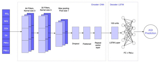
Figure 4.
CNN-LSTM architecture.
4.1.1. Encoder
In the proposed methodology, CNN act as an encoder with 64 and 32 feature maps per CNN layer and a kernel of size 3. The first CNN layer act as a filter to extract useful information from the input before generating the feature map. The second CNN layer repeats the same process, which improves the overall convolved feature map. The max-pooling layer simplifies the feature maps and generates a 1-Dimensional matrix.
In addition to that, the dropout and flatten layers are added to the encoder. The aim of adding the dropout layer is to prevent the model from overfitting while the flatten layer is added in the encoder to generate a long vector which can be used in the decoder (LSTM) as an input.
4.1.2. Decoder
The internal representation of the vector sequence is forwarded as an input to the LSTM. The LSTM is defined as a hidden layer of 100 units. Consequently, the whole sequence with each of the 100 units is generated as an output for each ambient air pollutant. The generated output will serve as the foundation for the prediction of AQI. Moreover, a fully connected (FC) layer is opted to comprehend the time series and make a prediction in the output. This was achieved by encapsulating the interpretation and output layers in a Temporal Distributed wrapper (TDW), which has been used for each decoder time step. This enables the LSTM to specify the context essential for each step in the output sequence, while the TDW dense layers interpret each time step uniquely while reusing identical weights.
4.2. IoT Monitoring Station Malfunction
IoT devices are vulnerable to battery drainage, failure or malfunction. This malfunction can occur due to many reasons such as equipment failure, integration problems, connectivity or device load. However, this failure can cause disruption of information from an MS to the system and directly affect the overall performance.
Henceforth, we presented an adaptive fault-tolerant framework to tackle this issue. The system, after regular intervals of time t checks the system for anomalies and failures. Once the system detects malfunction or anomalies from MS, it changes its status from to . The system computes geological position and creates a distance table (D) of the . We used IoT localisation [33] to identify the exact location () of the so that spatial interpolation can be applied. Furthermore, the longitude (℘) and latitude () information of are utilised to calculate the distance between and using Equation (10).
The one with the shortest distance to the became the candidate for as shown in Figure 5. A distance threshold is selected so that only the closest neighbouring can compete for the . This selection process of is done dynamically through context-aware sensing. Furthermore, a weightage is assigned to each based on distance proximity. The proposed framework integrates the historical air pollutants concentration () of with the current air pollutants concentration () of . The adaptive framework process is listed in Algorithm 1.
| Algorithm 1 Fault-tolerant Monitoring Station Framework |
|
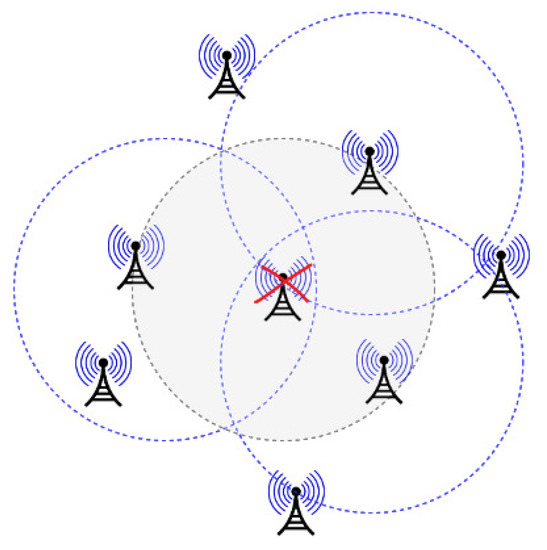
Figure 5.
Monitoring Station Election Process.
This amalgamation of and provides us insights into the correlations between the distance of multiple and its air pollutants concentrations. It gives a neighbourhood context-awareness which improves the overall prediction. Furthermore, this cross-grid area overlapping scheme can increase the system’s robustness and overall reliability.
4.3. Performance Evaluation Metrics
To make model results more intuitive and reliable, we performed a comparative analysis by employing MAE, MAPE and MSE with state-of-the-art frameworks such as Decision Tree (DT), Random Forest (RF), Support Vector Regression (SVR), Multilayer Perception (MLP), Long short-term Memory (LSTM) and Stacked Long short-term Memory (SLSTM). The MAE, MAPE and MSE are used to calculate the prediction error, and the lower the value means, the higher the prediction accuracy.The aforementioned performance metrics are calculated using Equations (11)–(13).
where X represent the real values while represent the predicted values of ambient pollutants.
5. Results and Discussion
This section is organised into two parts. In the first part, the results and predictions of the proposed model; CNN-LSTM, are presented. The results are compared with other state-of-the-art frameworks, whilst in the second part, we implement the monitoring station malfunction scenario and prediction results are compared with the actual real-time acquired results.
5.1. CNN-LSTM Prediction Model
The proposed model; CNN-LSTM, is evaluated for each pollutant element to check model efficacy and reliability. In experimentation, we forecast 7 days (from 25 December 2019 to 31 December 2019) of ambient air pollutants concentration on an hourly basis. Consequently, the predicted values of each ambient pollutant are compared with the real-time values to compute the error and experiment results (as illustrated in Figure 6). It is preeminent to state that the experimental results support our hypothesis to opt for the hybrid model, LSTM as a core network to resolve the long-term dependencies while using CNN to extract features and patterns for training and learning. The results support that the proposed CNN-LSTM model is very suitable for complex multivariate ambient pollutant scenarios.
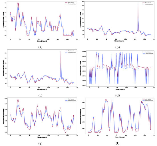
Figure 6.
Comparison result of Real and Predicted air pollutant concentration of (a) , (b) , (c) , (d) , (e) and (f) .
In particular, in the comparison experiment (as illustrated in Figure 6), it is clear that the accuracy of the proposed model is better adapted to the complex air quality data. The proposed CNN-LSTM model predicted the concentration of the pollutants with better fitting to the real-time concentrations by leveraging historical information. The proposed model is able to identify and predict, with a high degree of precision, the sudden rise in the concentration level of and (as shown in the Figure 6b,c). However, in the case of and , the model generates a trivial prediction latency (as shown in Figure 6d,e). This prediction latency occurred due to very smaller values like th and th, perpetual fluctuation and no temporal pattern. While in the case of and , the model predicts the air pollutant concentration with great precision and generates a very low prediction latency (as shown in Figure 6a,f).
Many research scholars have proposed the Stacked LSTM [7] or Nested LSTM model [17,19] to achieve better accuracy and prediction for ambient monitoring systems. However, SLSTM and NLSTM increase the overall computational cost and processing overhead. One of the major contributions of this paper is to propose a lightweight CNN-LSTM model for multivariate ambient pollution monitoring while achieving better accuracy and prediction.
The prediction results of each ambient pollutant are computed for state-of-the-art frameworks and detailed analysis. In comparison with the other state-of-the-art models (as shown in Figure 7), the proposed methodology has the best prediction performance. The proposed model outperforms all the compared state-of-the-art frameworks in terms of error and provides a better fitting to the real-time values with higher accuracy. There are several factors for this outcome. First, the CNN divides the complex air quality data into various components and extracts the best parameters. This efficient extraction of parameters improves the prediction performance of the LSTM, which improves the overall accuracy of the proposed model.
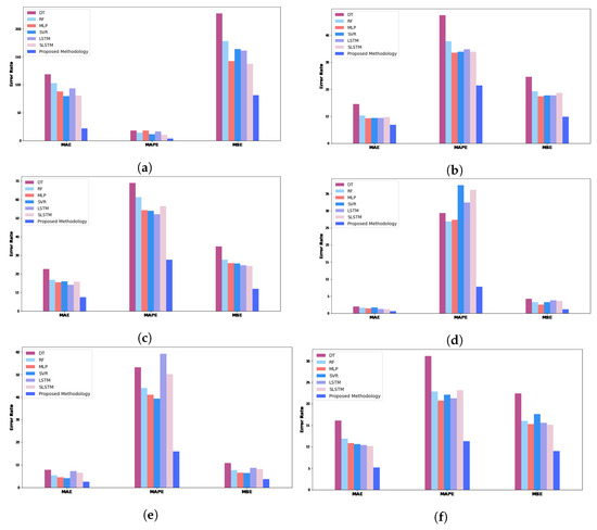
Figure 7.
Comparison Analysis of Proposed Framework prediction results with State-of-the-art Frameworks for (a) , (b) , (c) , (d) , (e) and (f) .
It is visible that the values of MAE, MSE and MAPE of the proposed model are significantly smaller in contrast with other compared frameworks. The proposed CNN-LSTM model generates MAE, MSE and MAPE of 0.63, 1.16 and 7.79 for SO2 which is an average of 57.33%, 65.23% and 74.96% lower than the state-of-the-art frameworks. Moreover, the values of MAE, MSE and MAPE generated by the proposed model are less than those of the other frameworks on an average of 54.80%, 52.78% and 60.02%.
In the case of PM2.5, the proposed CNN-LSTM model outperforms the LSTM and SLSTM by reducing 27.10% and 29.87% of MAE, 44.39% and 46.99% of MSE and 38.50% and 36.85% of MAPE values, respectively. Meanwhile, in the case of PM10, the model generates 7.54 MAE, 12.02 MSE and 27.61 MAPE which is almost 50% less than LSTM and SLSTM subsequently. An error table of MAE, MAPE and MSE for which pollutants is shown in the Appendix B.
The results validate the need for data preprocessing and efficient feature extraction procedures to create uniformity in the acquired dataset. Figure 7 illustrates that using CNN as an encoder or data preprocessor improves the overall prediction accuracy. Furthermore, the proposed CNN-LSTM model is able to predict the concentration of ambient pollutants very close to real-time concentration with a low prediction latency, which is used as a benchmark for AQI prediction.
Although the proposed model predicted air pollutants concentration with good accuracy, the results of this study can be further improved. Due to the limitations of air pollutant information regarding the border region MS and meteorological factors near the MS.
5.2. IoT Monitoring Station Malfunction
The inherent nature of IoT devices makes them vulnerable to malfunction or failure, which can affect the overall performance and information disruption. Henceforth, an adaptive fault-tolerant framework is proposed to address this issue. The proposed model uses the historical information on malfunction and leverages cross-grid neighbourhood information to predict ambient pollutants of that coverage area.
We evaluated the proposed algorithm for each pollutant element to check its robustness and reliability. For experimentation, we implemented the IoT-MS malfunction scenario at the Jung-gu station (as shown in Figure 8) and forecast 2 days (30 & 31 December 2019) of ambient pollution on an hourly basis. The results are compared with the real pollutant values of that area to observe the behaviour and overall performance scheme. We plot the output of the proposed scheme with the real values.
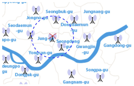
Figure 8.
Malfunction Monitoring Station and Election of Monitoring Station for Cooperative monitoring.
Figure 9 shows that the proposed scheme predicted the pollutant with better accuracy and precision due to its adaptive neighbourhood context-aware nature. This intrinsic nature provides robustness and improves the overall confidence in the system. Furthermore, it gives us a better understanding of the correlation between ambient pollutants and distance among .
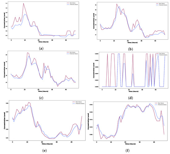
Figure 9.
Comparison result of Real and Predicted air pollutant concentration of (a) , (b) , (c) , (d) , (e) and (f) .
The proposed model predicts the concentration of air pollutants such as , and , with high accuracy and generates a very low prediction latency (as shown in Figure 9b,c,f). However, in the case of and , the model generates perpetual fluctuation and trivial prediction latency (as shown in Figure 9d,e). We employed MSE and MAPE to compute the error generated by the system and get a better understanding of the model behaviour. The results of each ambient pollutant element are summarised in Table 2. The proposed scheme generates a MAPE of 11.5% for whereas 7.99% and 7.62% for and respectively.The results show that the model predicted the ambient pollutant concentration with better fitting to the real data.

Table 2.
Prediction results in cooperative monitoring framework.
The results show that only those that are closer to malfunctioning should be selected for cooperative ambient pollutant prediction. Those which are at a distance from the malfunctioned can have very little effect since their ambient pollutant results are influenced by their neighbourhood. By electing far stationed can reduce the overall performance of the model. Henceforth, to tackle this issue, we introduced a distance threshold and assign weightage on a distance basis.
6. Conclusions
Air pollution has a significant impact on human health, daily life activities and the environment. Recently, a lot of research and studies have been done to monitor and mitigate the effect of deteriorating air quality. In this paper, a hybrid CNN-LSTM model is proposed to predict multivariate air pollutants for IoT-enabled environments.
In experimentation, a smart city (Seoul, Republic of Korea) dataset is acquired via various monitoring stations from January 2017 to December 2019. The proposed model provides a high degree of fitting to the real-time concentration of the ambient pollutants. The proposed CNN-LSTM model generate an average MAE, MAPE and MSE of 7.47%, 14.60% and 19.53%, respectively. The proposed model also outperforms various state-of-the-art models and illustrates visible excellence in terms of multivariate pollutant concentration prediction with an average of 54.80%, 52.78% and 60.02% in terms of MAE, MAPE and MSE. Moreover, the CNN-LSTM framework generates less error and prediction latency as compared to other state-of-the-art models.
In addition to that, an adaptive fault-tolerant framework is presented to make the air pollution monitoring system more robust and trustworthy. The adaptive framework exploits the interdependencies between multiple monitoring stations and pollutant concentration in those regions. Consequently, the model generates an average MAPE and MSE of 10.90% and 12.02%, respectively.
In the future, we will further investigate the impact of participatory sensing or mobile MS on air pollutant prediction. By using the predicted air pollutant concentration values, we will devise a mechanism to identify the perilous air quality areas and use that information for air pollution control.
Author Contributions
Conceptualisation, M.A.K., H.P. and H.-c.K.; methodology, M.A.K., H.P. and H.-c.K.; software, M.A.K.; validation, M.A.K.; formal analysis, M.A.K. and H.P.; investigation, M.A.K. and H.P.; resources, H.P. and H.-c.K.; data curation, M.A.K. and H.P.; writing—original draft preparation, M.A.K.; writing—review and editing, M.A.K., H.P. and H.-c.K.; visualisation, M.A.K. and H.P.; supervision, H.P. and H.-c.K.; project administration, H.P.; funding acquisition, H.P. All authors have read and agreed to the published version of the manuscript.
Funding
This research was funded by a 2021 Research Grant from Sangmyung University, South Korea.
Data Availability Statement
The data presented in this study are available upon request from the corresponding author.
Conflicts of Interest
The authors declare no conflict of interest.
Abbreviations
The following table describes the significance of various abbreviations and acronyms used throughout the paper:
| CO | Carbon monoixide |
| PM2.5 | Fine Particulate Matter |
| PM10 | Respirable Particulate Matter |
| SO2 | Sulfur dioxide |
| NO2 | Nitrogen dioxide |
| O3 | Ozone |
| NN | Neural Network |
| CNN | Convolutional Neural Network |
| LSTM | Long Short-Term Memory |
| ANN | Artificial Neural Network |
| RNN | Recurrent Neural Network |
| DT | Decision Tree |
| RF | Random Forest |
| SVR | Support Vector Regression |
| MLP | Multilayer Perception |
| SLSTM | Stacked Long Short-Term Memory |
| CNN-LSTM | Convolutional Neural Network integrated with Long Short-Term Memory |
| MS | Monitoring Station |
| IoT | Internet of Things |
| TDW | Temporal Distributed Wrapper |
| MSNorm | Normal Monitoring Station |
| MSMal | Malfunctioned Monitoring Station |
| MSElect | Elected Monitoring Station |
| MAE | Mean Absolute Error |
| MSE | Mean Square Error |
| MAPE | Mean Absolute Percentage Error |
Appendix A. Geographical Locations of IoT Monitoring Stations
| Sr. | Station Name | Longitude | Latitude |
| 1 | Jongno-gu | 37.572016 | 127.005008 |
| 2 | Jung-gu | 37.564263 | 126.974676 |
| 3 | Yongsan-gu | 37.540033 | 127.00485 |
| 4 | Eunpyeong-gu | 37.609823 | 126.934848 |
| 5 | Seodaemun-gu | 37.593742 | 126.949679 |
| 6 | Mapo-gu | 37.55558 | 126.905597 |
| 7 | Seongdong-gu | 37.541864 | 127.049659 |
| 8 | Gwangjin-gu | 37.54718 | 127.092493 |
| 9 | Dongdaemun-gu | 37.575743 | 127.028885 |
| 10 | Jungnang-gu | 37.584848 | 127.094023 |
| 11 | Seongbuk-gu | 37.606719 | 127.027279 |
| 12 | Gangbuk-gu | 37.64793 | 127.011952 |
| 13 | Dobong-gu | 37.654192 | 127.029088 |
| 14 | Nowon-gu | 37.658774 | 127.068505 |
| 15 | Yangcheon-gu | 37.525939 | 126.856603 |
| 16 | Gangseo-gu | 37.54464 | 126.835151 |
| 17 | Guro-gu | 37.498498 | 126.889692 |
| 18 | Geumcheon-gu | 37.452357 | 126.908296 |
| 19 | Yeongdeungpo-gu | 37.525007 | 126.89737 |
| 20 | Dongjak-gu | 37.480917 | 126.971481 |
| 21 | Gwanak-gu | 37.487355 | 126.927102 |
| 22 | Seocho-gu | 37.504547 | 126.994458 |
| 23 | Gangnam-gu | 37.517528 | 127.04747 |
| 24 | Songpa-gu | 37.502686 | 127.092509 |
| 25 | Gangdong-gu | 37.544962 | 127.136792 |
Appendix B. Comparison Analysis of Prediction Results with State-of-the-Art Frameworks
Appendix B.1. Prediction Result for CO
| Model | MAE | MAPE | MSE |
| DT | 118.71 | 18.25 | 227.94 |
| RF | 102.65 | 14.14 | 178.25 |
| SVR | 79.72 | 11.68 | 164.08 |
| MLP | 87.94 | 17.92 | 142.54 |
| LSTM | 93.18 | 16.63 | 161.02 |
| SLSTM | 80.6 | 10.29 | 137.73 |
| CNN-LSTM | 22.11 | 3.52 | 81.37 |
Appendix B.2. Prediction Result for PM2.5
| Model | MAE | MAPE | MSE |
| DT | 14.55 | 47.49 | 24.62 |
| RF | 10.34 | 37.76 | 19.22 |
| SVR | 9.42 | 33.93 | 17.74 |
| MLP | 9.22 | 33.54 | 17.43 |
| LSTM | 9.37 | 34.83 | 17.75 |
| SLSTM | 9.74 | 33.92 | 18.62 |
| CNN-LSTM | 6.83 | 21.42 | 9.87 |
Appendix B.3. Prediction Result for PM10
| Model | MAE | MAPE | MSE |
| DT | 22.63 | 69.03 | 34.79 |
| RF | 16.78 | 61.3 | 27.67 |
| SVR | 15.97 | 53.91 | 25.61 |
| MLP | 15.5 | 54.3 | 25.81 |
| LSTM | 14.17 | 52.2 | 24.68 |
| SLSTM | 15.83 | 56.55 | 24.29 |
| CNN-LSTM | 7.54 | 27.61 | 12.02 |
Appendix B.4. Prediction Result for SO2
| Model | MAE | MAPE | MSE |
| DT | 1.94 | 29.37 | 4.21 |
| RF | 1.64 | 26.92 | 3.26 |
| SVR | 1.71 | 37.55 | 3.21 |
| MLP | 1.42 | 27.39 | 2.49 |
| LSTM | 1.27 | 32.41 | 3.8 |
| SLSTM | 1.16 | 36.15 | 3.6 |
| CNN-LSTM | 0.63 | 7.79 | 1.16 |
Appendix B.5. Prediction Result for NO2
| Model | MAE | MAPE | MSE |
| DT | 7.81 | 53.18 | 10.87 |
| RF | 5.39 | 44.02 | 7.76 |
| SVR | 4.14 | 39.26 | 6.43 |
| MLP | 4.52 | 41.04 | 6.58 |
| LSTM | 7.32 | 59.26 | 8.72 |
| SLSTM | 6.51 | 50.18 | 8.11 |
| CNN-LSTM | 2.6 | 16.02 | 3.75 |
Appendix B.6. Prediction Result for O3
| Model | MAE | MAPE | MSE |
| DT | 16.09 | 31.18 | 22.42 |
| RF | 11.87 | 22.87 | 16.03 |
| SVR | 10.62 | 22.12 | 17.57 |
| MLP | 10.79 | 20.73 | 15.28 |
| LSTM | 10.39 | 21.32 | 15.57 |
| SLSTM | 10.16 | 23.16 | 15.11 |
| CNN-LSTM | 5.15 | 11.25 | 9.01 |
References
- World Health Organization. Ambient Air Pollution; World Health Organization (WHO): Geneva, Switzerland, 2021. [Google Scholar]
- World Health Organization. Household Air Pollution and Health; World Health Organization (WHO): Geneva, Switzerland, 2021. [Google Scholar]
- Kumar, A.; Goyal, P. Forecasting of daily air quality index in Delhi. Sci. Total. Environ. 2011, 409, 5517–5523. [Google Scholar] [CrossRef] [PubMed]
- Cheng, W.; Shen, Y.; Zhu, Y.; Huang, L. A neural attention model for urban air quality inference: Learning the weights of monitoring stations. In Proceedings of the Thirty-Second AAAI Conference on Artificial Intelligence, New Orleans, LA, USA, 2–7 February 2018. [Google Scholar]
- Rybarczyk, Y.; Zalakeviciute, R. Machine learning approaches for outdoor air quality modelling: A systematic review. Appl. Sci. 2018, 8, 2570. [Google Scholar] [CrossRef]
- Park, S.; Kim, M.; Kim, M.; Namgung, H.G.; Kim, K.T.; Cho, K.H.; Kwon, S.B. Predicting PM10 concentration in Seoul metropolitan subway stations using artificial neural network (ANN). J. Hazard. Mater. 2018, 341, 75–82. [Google Scholar] [CrossRef] [PubMed]
- Pak, U.; Kim, C.; Ryu, U.; Sok, K.; Pak, S. A hybrid model based on convolutional neural networks and long short-term memory for ozone concentration prediction. Air Qual. Atmos. Health 2018, 11, 883–895. [Google Scholar] [CrossRef]
- Garcia, J.; Teodoro, F.; Cerdeira, R.; Coelho, L.; Kumar, P.; Carvalho, M. Developing a methodology to predict PM10 concentrations in urban areas using generalized linear models. Environ. Technol. 2016, 37, 2316–2325. [Google Scholar] [CrossRef] [PubMed]
- Chen, J.; Lu, J.; Avise, J.C.; DaMassa, J.A.; Kleeman, M.J.; Kaduwela, A.P. Seasonal modeling of pm2.5 in California’s San Joaquin Valley. Atmos. Environ. 2014, 92, 182–190. [Google Scholar] [CrossRef]
- Truong, T.P.; Nguyen, D.T.; Truong, P.V. Design and Deployment of an IoT-Based Air Quality Monitoring System. Int. J. Environ. Sci. Dev. 2021, 12, 139–145. [Google Scholar] [CrossRef]
- Nasution, T.; Muchtar, M.; Simon, A. Designing an IoT-based air quality monitoring system. IOP Conf. Ser. Mater. Sci. Eng. 2019, 648, 012037. [Google Scholar] [CrossRef]
- Toma, C.; Alexandru, A.; Popa, M.; Zamfiroiu, A. IoT solution for smart cities’ pollution monitoring and the security challenges. Sensors 2019, 19, 3401. [Google Scholar] [CrossRef]
- Gupta, H.; Bhardwaj, D.; Agrawal, H.; Tikkiwal, V.A.; Kumar, A. An IoT based air pollution monitoring system for smart cities. In Proceedings of the 2019 IEEE International Conference on Sustainable Energy Technologies and Systems (ICSETS), Bhubaneswar, India, 26 February–1 March 2019; pp. 173–177. [Google Scholar]
- Zhang, J.; Zhong, C.; Yi, M. Did Olympic Games improve air quality in Beijing? Based on the synthetic control method. Environ. Econ. Policy Stud. 2016, 18, 21–39. [Google Scholar] [CrossRef]
- Wang, B.; Gu, X.; Yan, S. STCS: A practical solar radiation based temperature correction scheme in meteorological WSN. Int. J. Sens. Netw. 2018, 28, 22–33. [Google Scholar] [CrossRef]
- Chakma, A.; Vizena, B.; Cao, T.; Lin, J.; Zhang, J. Image-based air quality analysis using deep convolutional neural network. In Proceedings of the 2017 IEEE International Conference on Image Processing (ICIP), Beijing, China, 17–20 September 2017; pp. 3949–3952. [Google Scholar]
- Wang, B.; Kong, W.; Guan, H.; Xiong, N.N. Air quality forecasting based on gated recurrent long short term memory model in Internet of Things. IEEE Access 2019, 7, 69524–69534. [Google Scholar] [CrossRef]
- Spachos, P.; Hatzinakos, D. Real-time indoor carbon dioxide monitoring through cognitive wireless sensor networks. IEEE Sens. J. 2015, 16, 506–514. [Google Scholar] [CrossRef]
- Zhao, J.; Deng, F.; Cai, Y.; Chen, J. Long short-term memory-Fully connected (LSTM-FC) neural network for PM2.5 concentration prediction. Chemosphere 2019, 220, 486–492. [Google Scholar] [CrossRef]
- Wei, W.; Ramalho, O.; Malingre, L.; Sivanantham, S.; Little, J.C.; Mandin, C. Machine learning and statistical models for predicting indoor air quality. Indoor Air 2019, 29, 704–726. [Google Scholar] [CrossRef]
- Khan, M.A.; Kim, H.C.; Park, H. Exploiting Neural Network for Temporal Multi-variate Air Quality and Pollutant Prediction. J. Korea Multimed. Soc. 2022, 25, 440–449. [Google Scholar]
- Alawadi, S.; Mera, D.; Fernández-Delgado, M.; Alkhabbas, F.; Olsson, C.M.; Davidsson, P. A comparison of machine learning algorithms for forecasting indoor temperature in smart buildings. Energy Syst. 2020, 13, 689–705. [Google Scholar] [CrossRef]
- Rastogi, K.; Lohani, D.; Acharya, D. Context-Aware Monitoring and Control of Ventilation Rate in Indoor Environments Using Internet of Things. IEEE Internet Things J. 2021, 8, 9257–9267. [Google Scholar] [CrossRef]
- Tzortzakis, K.; Papafotis, K.; Sotiriadis, P.P. Wireless self powered environmental monitoring system for smart cities based on LoRa. In Proceedings of the 2017 Panhellenic Conference on Electronics and Telecommunications (PACET), Xanthi, Greece, 17–18 November 2017; pp. 1–4. [Google Scholar]
- Liu, S.; Xia, C.; Zhao, Z. A low-power real-time air quality monitoring system using LPWAN based on LoRa. In Proceedings of the 2016 13th IEEE International Conference on Solid-State and Integrated Circuit Technology (ICSICT), Hangzhou, China, 25–28 October 2016; pp. 379–381. [Google Scholar]
- Rossi, M.; Tosato, P. Energy neutral design of an IoT system for pollution monitoring. In Proceedings of the 2017 IEEE Workshop on Environmental, Energy, and Structural Monitoring Systems (EESMS), Milan, Italy, 24–25 July 2017; pp. 1–6. [Google Scholar]
- Zhang, D.; Woo, S.S. Real time localized air quality monitoring and prediction through mobile and fixed IoT sensing network. IEEE Access 2020, 8, 89584–89594. [Google Scholar] [CrossRef]
- Myeong, S.; Kim, Y.; Ahn, M.J. Smart city strategies—Technology push or culture pull? A case study exploration of Gimpo and Namyangju, South Korea. Smart Cities 2020, 4, 41–53. [Google Scholar] [CrossRef]
- How Seoul Is Struggling to Improve Its Air Quality. SmartCity: Expo World Congress 2. Available online: https://tomorrow.city/a/seoul-air-quality-improvement (accessed on 11 September 2022).
- Seoul Air Quality Index (AQI) and South Korea Air Pollution. IQAir. Available online: https://aqicn.org/city/seoul/ (accessed on 11 September 2022).
- Average Daily Atmospheric Environment Information by Period in Seoul. Seoul Open Data. Available online: https://dataportals.org/portal/seoul (accessed on 11 September 2022).
- Yan, R.; Liao, J.; Yang, J.; Sun, W.; Nong, M.; Li, F. Multi-hour and multi-site air quality index forecasting in Beijing using CNN, LSTM, CNN-LSTM, and spatiotemporal clustering. Expert Syst. Appl. 2021, 169, 114513. [Google Scholar] [CrossRef]
- Khan, M.A.; Khan, M.A.; Rahman, A.U.; Malik, A.W.; Khan, S.A. Exploiting cooperative sensing for accurate target tracking in industrial Internet of things. Int. J. Distrib. Sens. Netw. 2019, 15, 1550147719892203. [Google Scholar] [CrossRef]
Publisher’s Note: MDPI stays neutral with regard to jurisdictional claims in published maps and institutional affiliations. |
© 2022 by the authors. Licensee MDPI, Basel, Switzerland. This article is an open access article distributed under the terms and conditions of the Creative Commons Attribution (CC BY) license (https://creativecommons.org/licenses/by/4.0/).


