To solve the above problem, two modules—task clasification and buffering (TCB) and task offloading and optimal resource allocation (TOORA)—are modeled. The working process of these modules is given below.
4.1. Task Classification and Buffering (TCB)
Due to computation incapability of end devices, the tasks are transferred to nearest fog. The latency-sensitive tasks need to be processed first, thus these tasks are transferred to fog node. As noted above, the fog nodes are limited in resources and prediction of resource allocation is not immediately possible, that forced for buffering of tasks in the queue. If the queue length is long, then the time complexity is high. Similar to [
4], parallel virtual queues are considered for buffering the same type of tasks into separate virtual queues, which helps to reduce the time complexity, as shown in
Figure 3.
Theorem 1. Parallel virtual queues reduce the time complexity.
Proof. If a single queue with length M is considered for buffering tasks, then the time complexity for buffering all tasks is . If we consider four types of tasks that can be buffered in four separate virtual queues, then each queue length is . So, the time complexity is also decreased to . □
The real-time tasks
are streaming continuously from end devices and transferred to fog nodes. Each Task
can be represented with
, where
,
,
,
,
,
,
present arrival time, execution lower bound time, execution upper bound time, data size, number of instructions, response time, and deadline of the
ith task, respectively. Assume that the tasks arrive at fog nodes in equal time intervals. The
,
, and
of a task cannot be predicted before the task’s arrival. The execution time of the task is also not predicted before completion of the task. However, the upper and lower bounds of execution time (i.e.,
and
) can be estimated using machine learning algorithms proposed in [
49]. As per estimation,
should not exceed
. Here, we set
. Taking the above parameters of the task, the tasks can be classified into different types. The similar tasks can be grouped using a clustering algorithm. The tasks are overlapping, hence the FCM clustering algorithm is applied so that each task has a strong or weak association to the clusters. For the set of tasks
T, the association to each cluster can be calculated as follows:
where
n is the total tasks,
m is the fuzziness index
, and
represents the membership of the
ith task to
jth cluster center.
can minimize
when
and
for all
i and
j. Then
is
The cluster center can be calculated as
An iteration technique is applied until the minimum of
or minimum error criteria are satisfied. An error threshold
can satisfy the condition,
. The tasks are selected into a cluster using validity index. The Xie–Beni index [
27,
28]
is one of widely used validity index is used here and can be defined as
Fuzzy c-means cluster can classify the tasks for a given time interval
t. As the tasks are streaming continuously, dFCM [
27] is used adaptively to update cluster centers. A new cluster center is generated automatically with new cluster generation. Initially,
number of clusters are generated, where
. Upon arrival of new tasks, the membership of the present cluster is calculated. If the maximum membership value of the task exceeds or equals to membership threshold value (
), then it takes a new cluster center and generates a new cluster. Membership threshold (
) can avoid evaluation of cluster validity every time the tasks arrive. If the tasks satisfy the cluster membership, then there is no need to check for other, better clusters. The validity index is also evaluated when new centers are dissimilar to old ones. Then
can have the condition
Let
C number of clusters are there in time
t and maximum membership value of a task is lower than
then validity of clusters
C is compared with
to
. The clusters are generated using FCM and evaluated the validity index. The new cluster centers are generated for deviated tasks. This process is repeated to get the cluster center of best validity index until the arrival of tasks stop. The algorithm of task classification is as follows.
Algorithm 1 presents task classification using dFCM, which is discussed as follows. In this paper, an algorithm is presented using number of lines, and here, we consider the line number as a step. The parameters, such as threshold error , membership threshold , and range of c (i.e., number of clusters) are initialized in step-1. Here we are considering that tasks are coming in the same interval of time, hence is considered as the last interval. Time interval t is initialized with 0 in step-2, and the initial number of cluster c is in step-3. The following steps are computed until t reaches :
In step-5, take all the arrival tasks T in time t.
Calculate
c number of cluster centers, i.e.,
and
, using Equations (
6) and (
5); in steps 6 and 7.
In steps 8–20, check if the maximum membership value (i.e., ) of a task is more than or equal to membership threshold value (i.e., ). If true, then update and until , otherwise do steps 11–18 for to cluster centers. If no changes in clusters generated before then, store values of , otherwise generate new cluster for deviated tasks and update c. Then, update and until in step-20.
In step-21, compute validity index using Equation (
7) and select best clusters with best validity and assign to
in step-22.
Update the time interval t with t+1 in step-23.
Finally, return clusters of tasks in step-25.
| Algorithm 1 dFCM for task classification. |
Input: Continuous streaming tasks
Output: Cluster of tasks - 1:
Initialize , , , , , ; - 2:
; - 3:
; - 4:
while
do - 5:
Take a list of arrival tasks T at time t; - 6:
Compute c number of using Equation ( 6); - 7:
Compute using Equation ( 5); - 8:
if then - 9:
Update and until ; - 10:
else - 11:
for number of clusters from c − 2 to c + 2 do - 12:
if same number of clusters generated before then - 13:
Store values of ; - 14:
else - 15:
Generate new cluster center for deviated tasks; - 16:
; - 17:
end if - 18:
end for - 19:
Update and until ; - 20:
end if - 21:
Compute validity index using Equation ( 7); - 22:
; - 23:
; - 24:
end while - 25:
Return clusters of task ;
|
On basis of the number of clusters, that number of virtual queues are modeled for buffering the tasks. The task can be buffered in the queue by comparing the level of urgency that presents how much time a task can wait. The level of urgency of the task can be determined multiple ways. Here, we are considering deadline and laxity time, which are most useful for finding maximum waiting time from current time. The upper bound execution time is considered as actual execution time of a task cannot predict before completion of task. The waiting time of a task is calculated using laxity time as follows:
According to the lowest laxity time, the tasks can be buffered in different queues. However, some tasks may have the same
; those tasks are then grouped, and the earliest deadline first (EDF) time is considered for determining the waiting time. EDF of task
i is calculated as follows:
The algorithm for buffering the tasks in different queues is given below.
Algorithm 2 presents the task buffering in the queue that is discussed here. The results of Algorithm 1 are fed as the input of this algorithm (i.e., clusters of tasks). According to the number of clusters , that number of queues are created (i.e., Q) in step-1. The following steps are computed for each cluster .
Compute
using Equation (
9); for each task
in step-4.
Sort all the tasks according to in ascending order in step-6.
If any tasks have similar , then group them and store them in in step-8.
For each task of
, compute
using Equation (
10), and sort the tasks according to
in ascending order in steps 10–13.
Insert all the tasks in queue according to their and in step-14.
Finally, return the queues Q in step-16.
| Algorithm 2 Buffering task in queues. |
Input: Cluster of tasks
Output: Tasks buffered in queues Q- 1:
Take number of queues with number of clusters ; - 2:
for each cluster c in do - 3:
for each tasks in c do - 4:
Compute using Equation ( 9); - 5:
end for - 6:
Sort all the tasks according to in ascending order; - 7:
if some tasks having same then - 8:
tasks of same ; - 9:
end if - 10:
for each task in do - 11:
Compute using Equation ( 10); - 12:
Sort the task in according to in ascending order; - 13:
end for - 14:
Insert tasks of in queue according to their and ; - 15:
end for - 16:
Return Queues Q;
|
4.2. Task Offloading and Optimal Resource Allocation (TOORA)
The buffered tasks in virtual queues are going to be executed in either the cloud or fog node. The head tasks of each virtual queue are checked in parallel as to whether they will be executed in the cloud server or fog node or there may be a failure to achieve the deadline. The laxity time () of the task is used to determine the participation of the number of tasks of each queue for further operations.
The laxity time
of tasks in each queue are compared with the maximum laxity time of the head task of the queues; if the laxity time
of the task is below or equivalent to maximum laxity time of the head task, then those tasks are fetched for further processing, which can be represented as follows:
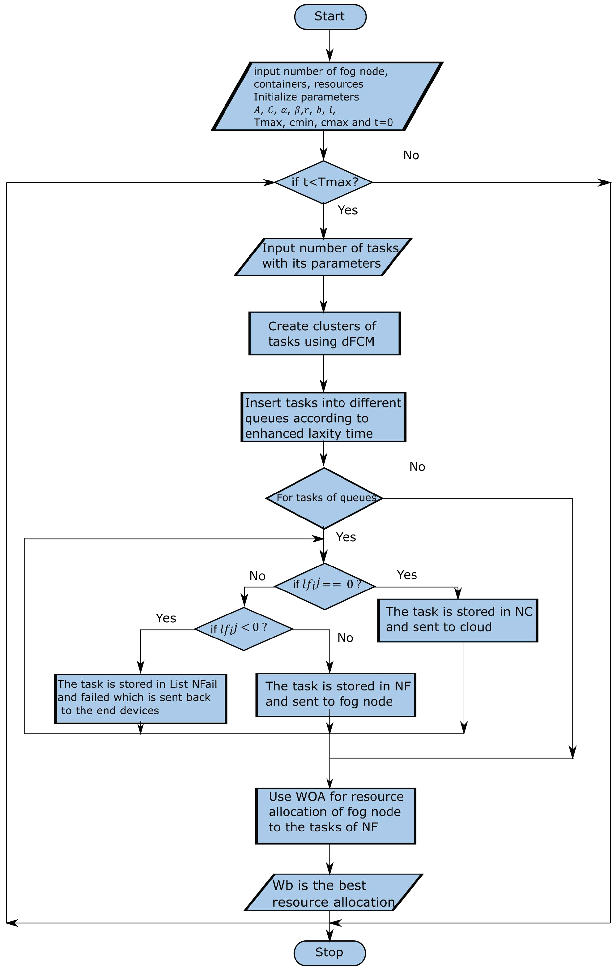
The fetched tasks from queues are further processed in TOORA for deciding whether the task will be offloaded or failed due to longer waiting time with three conditions as follows:
When , the deadline and executable upper bound time are nearly the same, so the task cannot wait for longer time to execute in fog node. therefore, the task must be moved to the cloud server for successful completion.
When , the executable upper bound time is more than the deadline, thus, the task cannot complete before the deadline and is sent back to end devices requesting to increase the deadline.
When , the task has enough time for executing successfully at the fog node before the deadline.
Algorithm 3 can be represented as follows for task offloading:
| Algorithm 3 Task offloading at fog node. |
Input:Tasks in -type queues
Output:Tasks at fog node , cloud and Failure task - 1:
for to do - 2:
Compute using Equation ( 11); - 3:
end for - 4:
for to do - 5:
for of do - 6:
if then - 7:
Remove from ; - 8:
; - 9:
end if - 10:
end for - 11:
end for - 12:
for i in TE do - 13:
if then - 14:
; - 15:
else if then - 16:
; - 17:
else - 18:
; - 19:
end if - 20:
end for - 21:
Return Queues , and ;
|
Algorithm 3 presents the task offloading at the fog node, which can distinguish the tasks of different types of queues. It takes all the tasks of -type queues and considers the tasks that are eligible for processing at that time. The number of tasks from each queue can be considered by computing steps 1–11. First, maximum laxity time of the head tasks of queues is computed in steps 1–3; next, the tasks from all -type queues whose laxity time is less than or equal to are selected and stored in list in steps 4–11. In steps 12–20, for each task in , check if laxity time of the ith task is equal to zero, then that task will send to the cloud server; if laxity time of the ith task is less than zero, then that task is marked as a failure and sent back to end devices for increasing the deadline; otherwise it will be executed in fog node. Finally, the tasks for fog node, the cloud, and failure are returned in step-21.
According to parallel virtual queues, let the number of tasks of type-
c queue in time slot
t be
and
. The tasks leave the queue when tasks are allocated resources in fog node or moved to the cloud server. The current length of type-
c queue in a given time can be evaluated based on total tasks arrived and removed from the queue at the previous time slot. If
is total tasks of type-
c that arrived, then the length of the queue can be evaluated as follows:
where
,
, and
contain total tasks that are moved to the cloud, tasks allocated for resources at fog node, and tasks that are failed at time slot
t.
To improve throughput and avoid starvation of tasks, the length of the
can be controlled using a Lyapunov function as follows:
The Lyapunov drift, a difference of the Lyapunov function of two slots, can be defined as follows:
Applying Equations (
13)–(
15), we can rewrite as follows:
The conditional expected Lyapunov drift can be represented as follows:
On basis of Lyapunov drift theory, if
is equivalent to zero or non-positive value, then the queue length is stable. The stability of queue depends on
. Although
,
, and
can influence the value of Equation (
16), the number of tasks in
and
are independent of tasks containing
. The tasks of
are allocated to the available resources of fog nodes and satisfied the following:
where
is the total ongoing tasks that cannot be released the resources in time
t. The objective of our work is to satisfy Equation (
17) and optimally allocate the resources. Most of the time meta-heuristic algorithms gives a near-optimal solution for the resource allocation problem [
15,
17]. Here, we are considering a meta-heuristic algorithm named whale optimization algorithm (WOA) [
50]. The main strategy of WOA is the hunting behavior of one species of whale called Humpback. Humpback whales use the unique feeding method named bubble-net feeding to create circle around the prey and spread bubbles, so that the prey move to nearer surface of the ocean, as shown in
Figure 4. The WOA get optimum solution using enclosing, bubble-net and explore methods.
In WOA, the random generated whale population are considered for optimization. These whales try to explore the location of prey and enclose them with bubble-net. During enclosing method, the whales upgrade their locations depending on best agent (i.e., target prey) as follows:
where
is the position vector difference of best agent (
and whales (
),
t is the present iteration, ⊗ is used for element-wise multiplication, and
and
are coefficient vectors and computed as
where every iteration decreases
from 2 to 0 linearly, and random vector
value lies in [0, 1]. The control parameter
can be improved as
(where
is the maximum iterations).
Equations (
20) and (
21) balance the exploration and exploitation. When
, exploration occurs, and exploitation occurs when
. During exploitation, the probability of getting location solutions can be avoided by taking parameter
as a random value in [0, 2].
The bubble-net method has two approaches: shrinking enclosing and spiral updating. The shrinking enclosing can be achieved by taking
in [−1, 1] with a linear decreasing value of
in each iteration. The spiral updating inspired with helix-shaped movement of Humpback whales is applied to update the position of the best agent and the whales as follows:
where a random generated
l value lies in [−1, 1] and
b is a constant used for logarithmic spiral shape.
The shrinking enclosing and spiral updating are performed simultaneously as whales move around the prey using both approaches. This behavior can be modeled by taking each approach with 50% probability as follows:
where
. When the coefficient vector
is greater than 1, the explore method is applied in which the whale location is replaced with a random whale rather than best agent. Thus, the algorithm can extend the search to a global search and can be represented as follows:
The bubble-net attach exploits the local solution from the current solution; whereas explore method tries to get a global solution from the population.
Here, we are considering WOA for allocating resources of fog nodes. Our whale optimized resource allocation (WORA) algorithm begins with generating a population of whales. Each whale denotes a random solution for a resource allocation problem. The fitness of each whale is calculated using a fitness function and selects a best solution with minimum fitness value as the current best agent. After this, the whales begin searching the global solution by updating each whale values of A, C, a, l, in each iteration. Where A and C are random coefficients, a is decreasing from 2 to 0 linearly, is [0, 1], and l is [2, 0]. Distance function is the most important function in WOA, which is designed for a continuous problem. As resource allocation problem is a discrete problem, the distance function can be modified. Whale creation, fitness function, and distance function as per our model is discussed below.
Whale creation: In our algorithm, each whale denotes a solution to the resource allocation problem. If we have a set of resources and a set of request tasks , then the whale can be represented as a random combination of resource with task . The resource is represented as , where f, c, r, , , and represent fog node, container of the fog node, resource block of the container, CPU usage, bandwidth, and available memory, respectively. The task can be represented as , which denote task identification number, requirement of CPU usage, bandwidth, and memory. For example,
Then a whale can be generated as follows:
=
=
=
In a similar fashion, all the whales are generated.
Fitness function: For each whale, the fitness function is the optimal resource allocation to the task and can be calculated as
The whale with minimum fitness is the optimum solution. Hence, the goal of the algorithm is the minimization of the fitness function.
The population can be generated by the collection of whales with their corresponding fitness.
Distance function: The most important function of WOA is the distance function. As three parameters (i.e., CPU usage, bandwidth, and memory) are considered, the distance function can be redefined as follows:
The WORA algorithm is given below.
Algorithm 4 presents assignment of fog resources to the tasks contained in . We initialize the whale population where , time t is 0, and the maximum iteration is in step-1. The best search agent that has minimum fitness value is identified in step-2. While t is less than , steps 3–21 are performed as follows:
For each whale, steps 4–16 are performed. The value of A, C, a, l, and are found in step 5.
If
is less than 0.5, then check the absolute value of
A in steps 6 and 7. If the absolute value of
A is less than 1, then update
D and
using Equations (
18), (
19), and (
29) in step 8. Otherwise, select a random whale
and update
D and
using Equations (
25), (
26), and (
29) in steps 10 and 11.
If
p is greater than 0.5, then update
and
using Equations (
22), (
23), and (
30) in step 14.
After updating, amend that goes beyond the search space in step 17. Then compute the fitness of all and update the best search agent with minimum fitness in steps 18 and 19.
Increment t by 1 in step 20.
Finally, return the best search agent that has optimal resource allocation to the tasks in step 22.
The complexity of an algorithm measures both space and time complexity. The space complexity is the amount of space occupied by the algorithm. In the WORA algorithm, the space complexity is related to the population size and the dimension of the problem. The population size is P and the dimension of the problem is D. Then, the space complexity is . In WORA, for , thus the space complexity is .
For time complexity, three major processes (i.e., initialization of the best whale, main loop for updating, and return of best solution) are considered. In WORA, is the maximum iterations.
Initializing the best whale takes times. The main loop updates the parameters, the whale that goes beyond the search space, and the optimum solution. The time complexity of these three stages are as follows:
Time required for updating the parameters is ;
Time required for searching whales beyond the search space is ;
Time for updating of optimal solution is ;
Time required for main loop is the sum of above the operations where and ignored;
The time required for last step .
Therefore, total time complexity of WORA algorithm is
.
| Algorithm 4 Whale optimized resource allocation (WORA) algorithm. |
Input: Set of resources R and tasks for fog node where
Output: Best solution for resource allocation - 1:
Initialize the whale population with , where , iteration , maximum iteration ; - 2:
Identify the best search agent ; - 3:
while
do - 4:
for k = 1 to P do - 5:
Amend A, C, a, l and ; - 6:
if then - 7:
if then - 8:
Amend D and by Equations ( 18), ( 19) and ( 29); - 9:
else - 10:
Choose a random whale ; - 11:
Amend D and by Equations ( 25), ( 26) and ( 29); - 12:
end if - 13:
else - 14:
Amend and by Equations ( 22), ( 23) and ( 30); - 15:
end if - 16:
end for - 17:
Amend that goes beyond the search space; - 18:
Compute fitness of whale ; - 19:
Update of best search agent; - 20:
; - 21:
end while - 22:
Return ;
|
The following lemmas [
51] are required for optimal convergence of the algorithm:
Lemma 1. The population of WOA supports Markov chain which is finite and homogeneous.
Lemma 2. The population of WOA absorb Markov process.
Lemma 3. If an individual of WOASU is stuck in local optima in the tth iteration, the transition probability of population is Lemma 4. The probability of convergence of WOASU algorithm towards the global optimal solution cannot possible.
Lemma 5. If an individual of WOAEP is stuck in the local optima in the tth iteration, the transition probability of population is Lemma 6. The WOAEP can converge in probability to the global optimum.
Lemma 7. WOA can converge in probability to the global optimum.
In the WORA algorithm, each whale represents random combination of resource with task as
. The valid whales, where the amount of
of resource is more than the requested task, can be considered for generating the populations. The fitness function, Equation (
27), calculates the average minimum difference of requested resource to allocated resource. Thus, the best whale is the whale that has the minimum fitness value. Using Lemmas 1–7, it is proved that WOA with spiral updating or enclosing method with probability of 50% can converge to a global optimum. Even if WOA is trapped to local optima by executing spiral updating mechanism, it can be come out from local optima using the enclosing mechanism. The WORA algorithm also adopts both spiral updating and enclosing method with 50% probability. Hence, the WORA algorithm can converge to global optima with probability to a point in infinite iterations.
The whole process of Algorithms 1–4 of our work is shown in the flowchart in
Figure 5.


 ,
, 


