Abstract
Mobile crowdsensing is considered as a promising technology to exploit the computing and sensing capabilities of the decentralized wireless sensor nodes. Typically, the quality of information obtained from crowdsensing is largely affected by various factors, such as the diverse requirements of crowdsensing tasks, the varying quality of information across different crowd workers, and the dynamic changes of channels conditions and the sensing environment. In this paper, considering the dynamics’ of the crowd workers, we focus on a spatial-temporal crowdsensing model and aim to maximize the value of information at the point of interest, by optimizing the recruiting range and time duration for the crowd workers. In particular, the crowdsensing system includes a mobile access point (MAP) and a set of wireless sensor nodes. As the information requester, the MAP can broadcast its crowdsensing task and then estimate the value of information by collecting the responses from the sensing nodes. Each sensing node in the crowdsensing task will receive a payment from the MAP. We aim to maximize the utility of the information requester by optimizing the recruiting range and waiting time for the sensing nodes. We firstly define a set of value metrics to characterize the MAP’s value of information. The optimal recruiting range can be obtained in closed-form expressions. Furthermore, considering the aging effect, we propose a gradient-based method to maximize the spatial-temporal value of information. Specifically, we first determine the optimal recruiting time for the requester and then choose the optimal recruiting range within each time slot. Via simulation, we first compare the sum, max, and min values of information at the requester, and then verify the effectiveness of the gradient-based method to optimize the recruiting time and range to maximize the value of information.
1. Introduction
Nowadays, with the popularization of smart devices and the development of modern wireless networks, people are increasingly engaged through mobile crowdsensing to collect, exchange, and aggregate various kinds of data for knowledge extraction that is beyond the capability of a single device [1,2,3]. Towards the future Internet of Things (IoT), the billions of smart devices provide not only means for communications and interaction, but they are also enhanced with various sensors, including cameras, microphone, global positioning system (GPS), Wi-Fi receivers, accelerometers, light sensors, etc., hence making it possible to extract context information easily. In particular, the cameras can be used as video and image sensors. The microphones are the acoustic sensors that can be used to estimate the ambient noise level. The GPS and Wi-Fi receivers can be used to estimate the device’s location or context information. The estimation of such context information becomes more accurate with the information provided by gyroscopes, accelerometers, proximity sensors, etc.
Mobile crowdsensing can leverage the decentralized smart devices and their sensors to acquire up-to-date information about a location (or event) of interest with a low cost. Typically, it is composed of the crowdsensing application or information requester that broadcasts the crowdsensing tasks and the mobile devices or crowd workers that are willing to participate in the crowdsensing tasks [4]. In some applications, it is difficult or costly to perform sensing tasks for information requesters at locations of interest, e.g., due to limited sensing capability or resource constraints. Instead, it can recruit nearby idle devices to perform the sensing task. The information acquired by a nearby device can be used by the information requester to gain environment awareness (e.g., traffic conditions in smart transportation system or spectrum vacancies in wireless communications). Hence, the performance of mobile crowdsensing largely relies on the spatial-temporal correlation of information at different devices. It offers excellent potential and unique qualities when considering and exploiting the user’s local information [5,6,7].
The information requester can assign the crowdsensing task to nearby crowd workers within a short distance sharing a similar spatial-temporal environment and, thus, potentially providing data with a higher reference value to the information requester. Previous field experiments have found that the information requester’s location and the recruiting range have a crucial impact when assigning crowdsensing tasks to the crowd workers [8,9,10,11,12]. Typically, the crowd workers are interested in participating in nearby crowdsensing tasks that are highly related to themselves, e.g., the reporting of traffic congestion information. They also prefer quick-to-solve crowdsensing tasks with the minimum efforts or resource consumption. The participation in nearby crowdsensing tasks also implies reduced costs in information exchange via wireless communications, which is crucial for low-power and low-cost IoT devices. This motivates the optimization of the information requester’s recruiting range for crowd workers. However, it is complicated by the diverse capabilities of crowd workers in different crowdsensing tasks and the uncertain quality of information provided by them, especially when the crowd workers are mobile devices with unpredictable channel conditions and sensing reliability. In addition, the crowd workers may have different expertise or preferences and, thus, only perform well in specific crowdsensing tasks.
Comparing to the previous works, in this paper we study a spatial-temporal crowdsensing system for a wireless sensor network considering both the uncertainty of information arrivals and the aging effect due to time delay between subsequent crowdsensing tasks. We focus on the spatial Poisson process to model the dynamic arrivals of crowd workers. The user arrival rate can be used to characterize the crowd workers’ preferences and capabilities in the crowdsensing task, e.g., a larger arrival rate means that more crowd workers are motivated and qualified with acceptable quality of information. Given such a stochastic model, we first define a few general-purpose performance metrics for the aggregated value of information at the information requester, including the sum-value, min-value, and max-value of information provided by all crowd workers. Then, we present closed-form representation for these performance metrics, which depend on the recruiting range and waiting time for the crowd workers’ responses. To this end, we aim to maximize the value of information at the information requester by optimizing the recruiting range and waiting time. Moreover, we extend the optimization problem into the multi-slot crowdsensing case, where the information requester can repeatedly recruit crowd workers to maintain information freshness. Considering the aging affect of information, we propose a gradient-based approach to maximize the information requester’s overall utility, by optimizing the waiting time between successive crowdsensing tasks. Our numerical results first compare different performance metrics at the information requester and examine the aggregated value of information with different recruiting range. We further verify the convergence of the gradient-based approach for optimizing the information requester’s crowdsensing scheduling strategy.
The remainder of this paper is organized as follows. We introduce some other related work in Section 2, we introduce the crowdsensing model in Section 3 and optimize the recruiting range of crowd workers in Section 4. In Section 5, we focus on the maximization of the aged value of information by optimally scheduling the information requests. Numerical results and conclusions are given in Section 6 and Section 7, respectively.
2. Related Works
To this end, numerous research works in literature have focused on modeling the crowd workers’ preferences, diverse crowdsensing task requirements, heterogeneous sensing capabilities, and the uncertainties in the quality of information in location-based spatial crowdsensing applications.
The authors in [8] proposed a novel framework that leverages the social media information to identify and select the crowd workers with specific domain expertise. The information requester can give more incentive to desirable crowd workers and motivate their participation. This framework was tested using a Flickr dataset and capable of gathering high-quality crowdsensing information without sacrificing fairness. The authors in [9] highlighted the limitation of monetary-based incentives in mobile crowdsourcing. Similar to [8], a location-based social network model was employed as a novel incentive mechanism to adjust task budgeting and ensure appropriate selection of crowd workers dynamically. The authors in [11] leveraged the computational cognitive modeling in mobile crowdsensing to improve campus safety. Drift-diffusion models were adopted to study the effect of different factors on crowd workers’ preferences and reporting tendencies in crowdsensing tasks. Considering a large set of different crowdsensing tasks, the authors in [10] studied the accurate and rapid allocation strategy of crowdsensing tasks to suitable crowd workers with different expertise and information quality. A real-time and budget-aware task package allocation strategy was proposed to improve the task allocation rate and simultaneously maximize the quality of information provided by crowd workers with limited budgets. The information requester needs to decide the set of crowd workers for each crowdsensing task, the reward for each task, and how the crowdsensing task is combined with other tasks. Instead of maximizing the immediate short-term rewards, the authors in [12] studied the cooperative task assignment by using multi-agent deep reinforcement learning approach that considers both the crowd workers’ and the information requesters’ long-term benefits.
In more practical cases, the crowd workers are independent, decentralized, and uncontrollable by the information requester. Thus, it becomes challenging to recruit a sufficient number of crowd workers with high-quality information. To motivate the crowd worker’s participation, the authors in [13] proposed a time and location correlation incentive scheme, which aims to collect the appropriate data and to satisfy the quality of information requirements with a minimum budget. The incentive scheme is shown to effectively improve the system performance by dynamically changing the reward for data samples based on the time and location of sensing data. The crowd worker’s mobility in a dynamic wireless network also brings uncertainty to the performance optimization of a mobile crowdsensing system. The authors in [14] assumed that the crowdsensing tasks with different quality requirements and the crowd workers with different capabilities both appear and leave dynamically in the crowdsensing system. A real-time online algorithm was proposed to solve the task assignment problem to maximize the total utility, without prior information about the crowdsensing tasks and the crowd workers. Considering time-constrained crowdsensing tasks and the moving crowd workers towards some direction, the authors in [15] aimed to assign crowd workers to different crowdsensing tasks, such that the completion reliability and the spatial/temporal diversities of the crowdsensing tasks are maximized. In addition to effective approximation approaches, e.g., the greedy, sampling, and divide-and-conquer algorithms, the authors further improved the efficiency by designing an effective cost-model-based index to dynamically maintain moving crowd workers and crowdsensing tasks with low cost. Predicting the appearance of crowdsensing tasks can potentially improve the performance of task assignment in spatial crowdsensing. This typically requires exact modeling and characterization of the spatial dependency among different points of interest and the temporal dependency at different time scales. The authors in [16] proposed a deep-learning-based prediction model to capture the temporal dependencies of historical task appearance at different time scales. Validated on the real-world dataset, the prediction model outperforms existing schemes when predicting crowdsensing tasks at hourly intervals, especially with intensive information requests.
However, the above-mentioned works seldom considered the aging of information due to the sensing and reporting delay in a dynamic wireless network. The aging of information has profound implications in wireless networks and has been extensively studied in the literature [17,18,19,20,21,22]. Many emerging applications, such as autonomous driving, interactive gaming, and virtual reality, depend on timely transmission and processing of the sensing data. The aging of information is used to characterize the information freshness in such time-sensitive applications. This concept can be also studied in spatial crowdsensing of a wireless sensor network. Ideally, the information requester aims to collect immediate responses from all crowd workers. Due to temporal correlation, the crowd workers’ immediate responses will provide the most relevant information to the requester and, thus, have the best quality of information. However, the distributed nature of crowd workers in a wireless sensor network implies that the time delay of information updates from individual crowd workers becomes stochastic. The crowd worker’s sensing information will arrive at the information requester randomly. Considering a dynamic network environment, the sensing information gradually becomes out of date or obsolete as the delay increases. Thus, a higher delay in the sensing information will introduce negative effect to the value of information at the requester. This can be modeled by the aging effect, which characterizes the rate of decreasing in the value of information. Moreover, to maintain an intimate understanding of the environment, the information requester may regularly send crowdsensing tasks to update context awareness. During two subsequent information updates, the context awareness will experience the aging effect, i.e., the value of information is decaying over time until the next information update. In spatial crowdsensing of a wireless sensor network, the wireless channel for information reporting is normally unreliable and difficult to predict accurately. Due to the aging of sensing information, the random delay will introduce uncertainty in the value of information at the information requester. In addition, the crowd workers may have limited energy resources. This makes it more difficult to incentivize the crowd workers and optimally schedule their information updates.
3. System Model
In this work, we consider location-based data acquisition in a wireless sensor network with a mobile access point (MAP) and a large set of wireless sensor nodes distributed over a geographical space (shown as Figure 1). The sensing information at individual nodes can be collected and jointly analyzed by the MAP, and then used for environmental monitoring and industrial surveillance. In particular, the MAP can be viewed as the information requester and deployed in a point of interest (PoI), broadcasting its sensing task and then collecting sensing information from nearby sensor nodes. The information collection from nearby sensor nodes will help the information requester quickly achieve location-aware context information at that PoI. For example, the decentralized sensing devices in environmental monitoring can report their local observations on temperature, humidity, wind direction, and speed levels to the MAP, which can help predict the risk of a wildfire and estimate its moving path in near future.
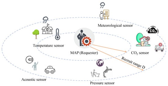
Figure 1.
Spatial-temporal value of information in a crowdsensing system.
Due to limited energy resource at individual sensing nodes, the information requester will give a payment to motivate the sensing nodes to participate in the crowdsensing task and report their local sensing information to the MAP. Hence, the information requester’s total payment depends on the how many sensing nodes are involved in the crowdsensing task. The MAP’s payment can be viewed as the cost for recruiting a set of sensing nodes. In particular, in energy-constrained wireless sensor networks, we assume that information requesters and all sensor nodes are equipped with energy transmitters and energy receivers, respectively. In many one-dimensional or vector models [23], the information requester can transmit RF power to all sensing nodes by transmitting RF signals, and most of the energy harvesting process obeys Rayleigh distribution [24,25]. Via energy harvesting, the energy-limited sensor nodes will become active and have sufficient energy to report their sensing information to the MAP. In this case, the information requester’s cost function relates to the overall energy consumption during the wireless power transfer to sustain the sensor nodes’ participation in the crowdsensing task [26,27].
3.1. Data Quality and Value of Information
The MAP can specify the recruiting range D and the time span T to collect sensing information from the sensor nodes. The recruiting range is a circular region centered at the PoI with the radius D. All sensor nodes in this area will perform the sensing task and report the sensing information to the MAP before the time deadline T. A larger D implies that the sensor nodes in a larger physical area can be employed in the task. In energy harvesting sensor networks, the time span T also determines the amount of wireless energy transfer to the sensor nodes given the MAP’s transmit power. Hence, a longer time span implies that more sensor nodes can become active and join in the crowdsensing task. From another aspect, the larger values of demands a higher transmit power at the MAP and more energy transfer time. This implies a higher energy cost of the MAP to recruit more sensor nodes. With limited energy budget at the MAP, it becomes a critical design problem to maximize the MAP’s utility by optimizing the time deadline T and the range parameter D to recruit a proper number of crowd workers in the crowdsensing task.
Let the PoI be the origin of coordinates and X be the random location of the sensor node in a two-dimensional (2D) space. The data quality of the sensor node is a function of the distance to the MAP or the data fusion center. Typically, as the distance increases, it will become less confident to estimate the true information at the location of the MAP. For example, when the sensor nodes are used to estimate the temperature at the PoI. The nearby sensor nodes will provide more reliable estimation. As such, we define the data quality received by the MAP as a decreasing function as follows:
where is a parameter describing the spatial correlation and ℓ is a constant parameter denoting the sensor node’s reliability in the sensing task. When approaches zero, the value approximates the value of truth. Larger means that the sensing environment is highly dynamic.
The information fusion at the MAP is based on a joint processing of all the information collected from different sensor nodes, which can be viewed as a function of individual sensor nodes’ data quality. Specifically, we propose different value functions as follows to model the information requester’s payoff by using crowdsourcing under different application scenarios [4].
- Sum Value: The MAP collects all information from the sensor nodes to make the final decision. The MAP’s payoff is defined as the sum of quality values of all active sensor nodes in the crowdsensing task, i.e.,where denotes the spatial Poisson process given the recruiting range D and the time span T, and n is the total number of all participating sensor nodes. Each item represents the location of the i-th active sensor node reporting its sensing information. This sum utility model is applicable for risk-neutral applications where the MAP equally aggregates all sensors’ information. The mean value of all sensor nodes’ quality values is used as an unbiased estimation of the value of information at the MAP. For example, in cognitive radio networks, the spectrum sensing task of a cognitive transmitter (i.e., the information requester) can be jointly performed by a set of nearby cognitive radios or sensor nodes. By aggregating the spectrum sensing results, the information requester can make a more reliable estimation on the availability of spectrum vacancies at the PoI.
- Max Value: When the information requester is risk-seeking, it will be optimistic for the information requester to take the maximum value of the data quality values reported by different sensor nodes. In this case, we define the MAP’s payoff as follows:In spectrum sensing of cognitive radio networks, this model corresponds to the “OR”-rule data fusion strategy. The data quality of each sensor node can be restricted in the set and viewed as a probabilistic indication of the channel occupancy. A larger value of means that the sensor node anticipates the spectrum vacancy with a higher probability. The max-value in (3) implies that the MAP would like to take a higher risk of collision to exploit the licensed channels more aggressively.
- Min Value: In contrast to the max-value in (3), it is risk-aversion for the information requester to seek the minimum of all crowd workers’ data quality values as its payoff:In this case, the information requester becomes sensitive or vulnerable to the worst-case data quality. This is similar to the “AND”-rule data fusion strategy in spectrum sensing of cognitive radio networks. The min-value in (4) implies that the information requester will output the value “0” (i.e., the spectrum is occupied at the PoI) if any sensor node detects a busy spectrum and reported “0” to the information requester. In this case, the information requester becomes very sensitive to the presence of the licensed users. Another example is to detect wildfire by deploying a set of wireless sensor nodes. The information requester will alarm if any sensor node detects the abnormal smoke or temperature.
3.2. Cost Function and the Overall Utility
The utility of the information requester can be defined as the difference between the payoff and the cost value for recruiting the sensor nodes, e.g., the price paid to individual sensor nodes or the wireless power transfer to sustain their operations. The cost function depends on the number of participating sensor nodes, given the recruiting range D and time span T. Taking sum-value as an example, the information requester’s utility function is given as follows:
where c is a constant weight parameter and defines the total price paid to all active sensor nodes given the parameter . We can simply define as linearly proportional to the number of active sensor nodes as follows:
where denotes the constant user arrival rate in the recruiting time T. The production can be viewed as the density of sensor nodes in the circular region centered at the MAP. As such, the constant parameter c can be viewed as the unit price paid to each sensor node. A larger D implies that more sensor nodes in a larger geographical area can be employed in the crowdsensing task. It is clear that both the payoff function and the cost value are increasing in terms of the range D, which implies the spatial-temporal trade-off when the information requester aims to maximize its utility.
Considering the wireless powered sensor network as a special case, the MAP’s cost depends on the power consumption to activate the sensor nodes. Given the range parameter D and the MAP’s transmit power , the received signal power at the cell-edge sensor nodes is given by , where n denotes the path loss exponent. By using an energy harvesting circuit, the RF power can be converted into DC power with the efficiency and stored in the sensor nodes’ batteries or capacitors. Typically, we require to activate the RF energy harvesters of sensor nodes. Hence, the MAP has to set its transmit power as to recruit all sensor nodes within the range D. During the recruiting time T, all sensor nodes harvest RF energy from the MAP and report their sensing information at the end of the recruiting time T. Hence, the MAP’s overall energy consumption during the recruiting time T is given as follows:
In this case, we can replace the cost function in (6) by the MAP’s overall energy consumption . It is clear that and have a similar form, as they are both increasing with respect to . Considering a simple free-space outdoor channel model, i.e., , both cost functions are linear in T and quadratic in D. In the sequel, we focus on the general cost model in (6) and derive the optimal recruiting parameters for the information requester.
4. Optimal Recruiting Range of Sensor Nodes
In the sequel, we first derive closed-form expressions for the information requester’s utility with different value functions. Then, given the waiting time T, we can determine the optimal recruiting range D in different cases. Further, in Section 5, considering the aging value of information, we investigate the interplay between the waiting time T and the recruiting range D, and propose an iterative procedure to optimize that maximizes the information requester’s utility.
4.1. Sum-Value Maximization
We first consider the sum-value function at the information requester. Note that the expectation in (2) is taken over all possible realization of the Poisson point process . Given the recruiting time T and the user arrival rate , by Campbell’s theorem, the sum-value in (2) can be rewritten as follows:
where denotes the circular region centered at the origin with radius D. The function is the intensity measure, which can be interpreted as the average number of points of the point process located in the two-dimensional region . denotes the average user arrival rate during the recruiting time T. Hence, represents the density of participating sensor nodes within the recruiting range D. If is time-invariant, we have for .
Given the exponential decreasing quality function in (1), the sum-value payoff in (8) can be simplified as follows:
where we define the constant for notational convenience. It is obvious that when or . This implies that there will be no sensor node responding to the information requester if we set either or . As the recruiting range D approaches infinity, the limiting value of is given as follows:
This limiting value implies that, for fixed recruiting time T, it is not always rewarding to increase the recruiting range D. A large D implies that more sensor nodes will provide their local information to the information requester. However, as the quality of information is a decreasing function of the distance to the information requester, the local information provided by a distant sensor node will have trivial contribution to the sum value of information accumulated by the information requester. For example, in spectrum sensing of cognitive radios, the spectrum environment can be similar for two nearby cognitive radios. We can infer the spectrum occupancy status by the sensing information provided by a nearby sensor node. However, when the distance between them is increasing, the spectrum information at one node will be of little referential value to the other.
In another aspect, as the recruiting range D increases, the total number of participating sensor nodes also increases, so does the information requester’s total payment to the sensor nodes. To ensure a cost-effective crowdsensing service, the information requester is motivated to maximize the information requester’s utility as follows:
Proposition 1.
The optimal to problem (10) is given by
The proof of Proposition 1 is given by Appendix A.1. Though the sum-value utility in (10) is an increasing function of the user arrival rate , the optimal recruiting range is independent with respect to , which enables the information requester to make the optimal decision without knowing the context information. A more general case is that the participating sensor nodes may be classified into multiple groups with different cost and quality values. In this case, the unit price c in (11) can be viewed as the averaged price paid to different sensor nodes. In particular, assuming that the participating sensor nodes are classified into W groups with different arrival rate and unit price for , the optimal recruiting range that maximizes the sum-value utility can be determined as follows:
Another observation from (11) and (12) is that the optimal recruiting range in the sum-value utility is independent of the time span T. As indicated in the objective of (10), both the payoff and the cost functions of the information requester are linear with respect to the time span T. With a longer waiting time T, the information requester will collect more information from the emerging sensor nodes during this period. Hence, the information requester’s payoff will increase by the summation of all users’ value of information. Meanwhile, the cost paid to all sensor nodes also increase linearly with respect to the number of sensor nodes. However, this result only holds if the value of information provided by individual sensor node does not fade with time, i.e., the historic sensing information provided earlier by the sensor node has the same importance as that of the more recent sensing information.
4.2. Max- or Min-Value Maximization
Given the recruiting parameters , the max- and min-value functions, denoted as and , respectively, have a similar structure as that in (8), and, hence, can be simplified in a similar way. Specifically, let denote the maximum value of the Poisson point process in a circular region with the radius D. Then, the max-value function can be derived by the following integration:
which can be further simplified by the following proposition.
Proposition 2.
The max- and min-value functions can be simplified as follows, respectively:
The proof of Proposition 2 is detailed in Appendix A.2. Note that the sensor node’s data quality decreases with the increase in the distance to the information requester. As the recruiting range D increases, those distant sensor nodes will poison the overall value of information at the information requester. The optimal recruiting range for the max- or min-value case can be obtained by solving the utility maximization problem similar to that in (10). Instead of a linear payoff function in (10), the optimizations for the max- and min-value cases involve non-linear and non-convex payoff functions and , as shown in (13) and (14). Given the time span T, we have the following propositions to optimize the recruiting range D.
Proposition 3.
Assuming the unit recruiting time , the optimal recruiting range that maximizes the max-value utility function is given as follows:
The proof of Proposition 3 is straightforward by checking the derivatives of the utility function. The first- and second-order derivatives of the max-value utility are given as follows:
Hence, the optimal recruiting range D is the the unique solution to , which easily leads to the result in (15). We can easily verify that by an inspection on (11) and (15).
Similarly, let denote the optimal solution to maximize the min-value utility . Though there is no closed-form expression for , we can easily determine it by a bisection method as revealed by the following proposition.
Proposition 4.
Given the unit recruiting time , the min-value utility is increasing in and decreasing in . Hence, there exist unique solution to maximize the min-value utility .
The proof of Proposition 4 is similar to that of Proposition 3. The details are omitted for brevity.
5. Maximizing Aged Value of Information
In previous section, we assume that the information requester recruits sensor nodes in a fixed time period . Given the recruiting range D, the number of sensor nodes are uniquely determined by the sensor nodes’ arrival rate in the circular region . In a dynamic environment, the sensor nodes may randomly move in or move out of the circular region. In addition, the availability of sensor nodes within the recruiting range D depends on the MAP’s wireless power transfer in the recruiting time T. All active sensor nodes in the spatial-temporal recruiting window will provide their sensing information to the information requester. A larger recruiting time T means that the information requester can wait for a longer time for crowd workers, however, with a higher cost paid to all sensor nodes. In addition, considering the aging effect of information [19,20,21], the information may become obsolete with a longer waiting time. We expect that the temporal correlation of sensing information collected at different time stamps decreases as time goes by, especially in a dynamic network environment.
In this part, we aim to determine the optimal recruiting time for the information requester to recruit sensor nodes. We assume a time-slotted frame structure for the information requester to broadcast its crowd sensing tasks and recruit the sensor nodes periodically. Each time slot is divided into two parts. The first sub-slot is used to recruit sensor nodes and wait for them to report their sensing information at the end of the sub-slot. In the second sub-slot, the information requester extract values (e.g., the sum-, max-, or min-value of information) from all local sensing information. The information requester will keep the value of information until the next time slot, when new sensing information is updated by the sensor nodes.
5.1. Aging Value of Information
Let denote the size of the k-th time slot. At the beginning of the time slot , the information requester extracts the value of information based on the collected information from all the sensor nodes recruited in previous time slot . The information requester also broadcasts its sensing task and recruits the active sensor nodes during the current time slot in Figure 2. It is clear that the time slot also represents the time interval between two successive crowd sensing tasks of the information requester. A larger time interval implies that more sensing information will be collected from the sensor nodes, but also a higher payment to the sensor nodes.
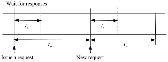
Figure 2.
A time-slotted structure for broadcasting periodical crowdsensing tasks and waiting for the crowd workers’ responses.
The extracted value of information at the beginning of the k-th time slot may become out-of-date gradually until the next time slot. The obsolete information will have little value to the information requester. For example, in spectrum sensing of cognitive radio networks, the collaborative sensing result of different sensor nodes will be valid only in a small time window due to the dynamics of spectrum activities. To model the freshness of information, we introduce a linear aging function to model the decreasing value of information as time goes by:
where the parameter controls the rate of decreasing value of information. During the time interval , the value of information is gradually decreasing as time goes by since the last information update. Let denote the value of information at the beginning of the k-th time slot, the aging value of information is given as follows:
A larger time slot allows the information requester to recruit more sensor nodes for the next time slot. However, it also leads to a decreasing value of information due to the aging effect in the current time slot. Given the value of information at the beginning of the k-th time slot, the aging value will last till the -th time slot. The evolution of the information requester’s aging value of information is illustrated in Figure 3.
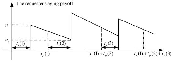
Figure 3.
The information requester’s aging value of information.
Considering the aging effect, the averaged value of information relates to both and , as shown in Figure 3. As such, the optimization of each time slot for crowdsensing becomes more complicated, especially with time-varying user arrival rate . Assuming the linear aging function, the information requester’s payoff function in each time slot can be defined by the time-averaged value of information as follows:
where represents the average linear aging coefficient and denotes the start time of the k-th time slot. Note that the initial payoff may take different forms depending on the fusion rules at the information requester, e.g., the sum-, max-, or min-value of information. The information requester’s cost function in the k-th time slot is linearly proportional to the number of sensor nodes recruited during the previous time slot . Given the recruiting range D, the total number of sensor nodes can be evaluated by
where denotes the average user arrival rate during the time slot .
5.2. Maximizing the Aged Sum-Value of Information
Considering the aging of the sum-value of information, we aim to maximize the overall value of information accumulated in N time slots:
where denotes the set of all feasible time allocation strategies in N time slots during the whole time horizon T. For sum-value of information, the payoff function can be rewritten as follows, similar to that in (9).
where we define and for notational simplicity. Then, we can reformulate the utility maximization problem in (17) as follows:
Note that , where is the time-averaged user arrival rate over the entire time horizon T, i.e., . Hence, we can further revise the aged sum-value utility in the objective of (19) as follows:
where we define and for notational convenience. We can observe that the optimization of recruiting time is coupled with the previous time slot in a non-convex structure. Though a direct solution to (20) is not available, we have the following proposition to explore its structural property.
Proposition 5.
Considering linear aging effect, problem (20) is non-negative and non-decreasing in for .
Proof.
The proof of Proposition (5) is straightforward by evaluating the first-order derivative of with respect to . With the linear aging function , we can firstly simply as follows:
Note that and it is increasing when . It is clear that is also non-negative and increasing in . In addition, we have , which is obviously increasing in . Now we can simplify the derivative of w.r.t as follows:
□
Proposition 5 implies that the utility will increase by increasing the length of each time slot. However, as we require , this brings the trade-off between different time slots. We can bypass this difficulty by verifying that the feasible region is obviously a normal set, i.e., for any , we always have if . This implies that we can use the monotonic optimization (MO) algorithm to solve the utility maximization problem in (19) optimally. The detailed procedures of the MO algorithm can be referred to [28] and omitted here for conciseness.
5.3. Maximizing the Aged Max- and Min-Value of Information
The aged max- and min-value utility maximization can be processed following a similar procedure as that for problem (17). Specifically, substituting into (17), the aged max-value utility maximization can be simplified as follows:
where we define for simplicity. It is clear that the objective in (21) is non-convex and complicated to analyze. In addition, different from the sum-value utility, the monotonicity in Proposition 5 fails to hold in this case. Fortunately, we can derive a lower bound on (21) by relaxing the coefficient to , defined as follows:
It is clear that for . By substituting into (21), a lower bound can be derived as an approximation to the maximum of problem (21). Moreover, the approximate utility maximization problem also has the appealing monotonicity similar to that in Proposition 5.
Proposition 6.
Replacing by , the objective in (21) becomes increasing in for .
Proof.
The proof of Proposition 6 needs to verify a non-negative derivative w.r.t. . Let denote the aged max-value utility in (21) with the approximation . Thus, we have the derivative as follows:
Note that both and are non-negative. We can focus on . By the definition of , we have and then the derivative can be simplified as follows:
where we define as follows for simplicity:
Till this point, we can ensure by showing that the coefficient is non-negative. Note that we always have the following inequality
for any x. This can be verified as follows:
Therefore, we have . This result ensures and thus we have . □
Similar to the aged max-value utility, substituting into (17), we can also devise a lower bound approximation to the aged min-value utility maximization problem as follows:
where . Similar to (22), a lower bound approximation to (24) can be found by revising the coefficient as follows:
Some manipulations reveal the following equalities:
which implies the non-negative derivative as follows:
Till this point, we conclude the the lower bound approximations to both problems (21) and (24) are monotonically increasing w.r.t the recruiting time vector , similar for the sum-value utility in Proposition 5. Therefore, the optimal solution to (21) and (24) can be similarly obtained in an iterative manner by using the MO algorithm.
5.4. A Gradient-Based Solution
The computational complexity of the MO algorithm increases rapidly with the size of decision variables in (19), (21), and (24). Hence, it becomes very inefficient as the number of time slots is increasing. In addition to the MO algorithm, we can also devise a gradient-based method with reduced computational complexity to search for a sub-optimal slot-time allocation strategy [29]. Considering the sum-value utility maximization, the optimal solution to (19) should satisfy the following property:
Proposition 7.
At the optimum of problem (19), we can verify that equals to some constant for all .
The conclusion in Proposition 7 is quite intuitive. As the objective is non-decreasing in each , once we find some , such that , we can further increase the objective function by simply increasing while decreasing by the same small quantity . The design of a gradient-based search algorithm relies on a primal-dual decomposition of (19). Specifically, introducing a non-negative dual variable , we can include the time allocation constraint as a penalty term into the objective and formulate the Lagrangian function as follows [30]:
where for simplicity. Given the dual variable , we first optimize each time slot to improve the Lagrangian function following the gradient direction. The gradient-based update of in each iteration is given as follows:
where denotes a small step-size in the -th iteration. The gradient of the Lagrangian function is given as follows:
Given the initial value , we can start the iteration from and update one by one. When the iterations traverse all , we turn to minimize the Lagrangian function by updating the dual variable , similarly following the gradient descent direction, i.e.,
where denotes the small step-size to update . With the new dual variable , we can start a new round of iteration to update the time allocation strategy. This process continues till and converge to stable values.
Further we consider a special case to problem (19), i.e., the information requester has only one information request during the time period T. The information requester has to decide how to set the recruiting time that maximizes the aged utility during the time period T. Focusing on the sum-value of information, the utility maximization in (19) is degenerated to the following problem:
where can be viewed as a constant. Note that and . The first- and second-order derivatives of w.r.t. are given as follows:
It is easy to verify by evaluating the first- and second-order derivatives of . By definition, for linear aging function we have
Thus, we have for and for . Therefore, we have and .
When , we have . In this case, the optimal time allocation is given by and . This implies that the information requester will collect all sensing information at the beginning of the time frame T. In the other case, when , we have and we can observe that is decreasing as increases. Hence, the optimal can be obtained at the stationary point of . Substituting and into , we have , which becomes a quadratic equation. Therefore, we can find easily by setting . Combining two cases, the optimal solution to (27) is given as follows:
For the max-value case, the aged utility maximization in (21) is degenerated as follows:
where the coefficient also relates to as we have . Though the first-order derivative of can be complex to analyze and closed-form optimal solution is not available, we can easily determine the optimal value by applying the primal-dual gradient updates in (25) and (26). The same result is also applicable to the min-value utility maximization problem.
6. Numerical and Simulation Results
In this part, we numerically evaluate the proposed crowdsensing strategy. The simulation experiments are conducted on AMD R7, 16 GB memory, 3.6 GHz CPU, using Python as the design language. We first illustrate different curves for the value of information and their limiting values at the information requesting. Then, to maximize the value of information in the second part, we are motivated to optimize the optimal recruiting parameters, including the waiting time and recruiting range for crowd workers. We also verify the general gradient-based approach for utility maximization, considering the aging effect in the value of information at the information requester. The constant parameter ℓ defined in (1) denotes the sensor node’s reliability in the crowdsensing task. We assume for all sensor nodes and focus on the heterogeneity of the computing and communication environments. We set to denote the spatial correlation of information at different locations. The weight parameter denotes the unit price paid to each active sensor node.
6.1. Utility Curves with Different Recruiting Range
Figure 4 illustrates the information requester’s utilities with different user arrival rates. A larger user arrival rate implies the higher density of crowd workers within the recruiting range. A direct comparison in Figure 4 reveals that the information requester’s utilities in either cases, i.e., the sum-, max-, and min-value cases, all increase with the density of crowd workers. In particular, with the smallest user arrival rate , the maximum sum-value of information is limited around 0.03, while this value increases up to 0.3 when we increase the user arrival rate to .
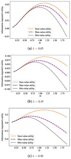
Figure 4.
The information requester’s utilities with the sum-, max-, and min-value of information, respectively.
As the recruiting range D increases, the information requester’s utilities show a similar trend in different cases, i.e., the utilities firstly increase and then decrease. The monotonicity of the utility curves is difficult to analyze. However, we can observe that there is an optimal recruiting range for the information requester to achieve its maximum utility. When the recruiting range is beyond the optimal value, the information requester’s utility begins to decrease with D gradually. The reason is that the delay for data transmission will be significant and the costs paid to all crowd workers also become excessive when the recruiting range is too large. Considering the spatial correlation in the value of information, a distant crowd worker will have poor data quality and thus less value of information. Therefore, by increasing the recruiting range, the information requester will obtain little payoff from the distant crowd workers but still pay the same price. This implies the diminishing utility as the recruiting range increases. The sum-value utility is risk neutral and, thus, it cumulates all crowd workers’ information. Therefore, we observe that the sum-value utility achieves the highest value of information compared with the max- and min-value utilities in Figure 5. To observe the effect of the parameter ℓ on the data quality function, Figure 6 shows that when the value of ℓ is larger, the variation range of the optimal range D also increases. Then, the gap between the optimal ranges D of the three different cases also increases. From this we can see that the parameter ℓ has a significant impact on the distance sensitivity.
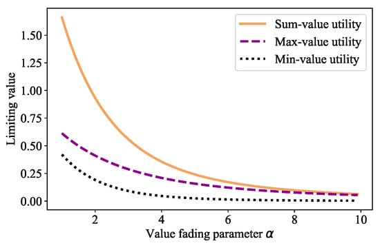
Figure 5.
Comparison of sum-, max-, and min-value of payoff.
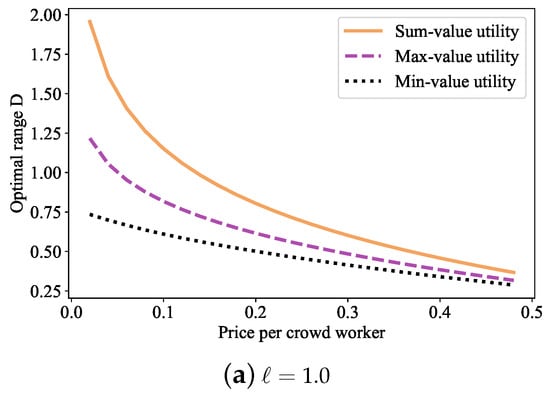
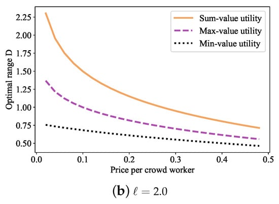
Figure 6.
The optimal recruiting range with different parameter ℓ.
In addition, the max-value utility is higher than that of the min-value utility. An interesting observation is that the optimal recruiting range in the max-value utility is not necessarily larger than that corresponds to the min-value utility. Figure 7 compares the optimal recruiting range with different utilities and unit prices c paid to each crowd worker. It shows that the optimal range for the sum-value utility is the largest one, compared to the max- and min-value utilities. The optimal recruiting range for the min-value utility is generally less than that for the max-value utility. However, we can find that, when lambda is less than or equal to 0.15, the optimal recruiting range for the max-value utility is less than that for the min-value utility. As the unit price c increases, the optimal recruiting ranges in all cases are decreasing. A higher price c implies that the information requester will be more cautious to increase its recruiting range due to the decreasing payoff obtained from distant crowd workers.
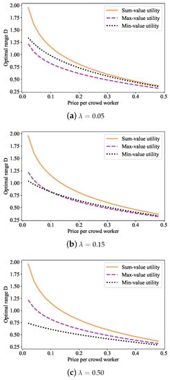
Figure 7.
The optimal recruiting range with different utilities.
6.2. Utility Maximization with Aging Value of Information
In this part, we evaluate the optimal recruiting time considering the linear aging effect. Given the recruiting range D, the optimization of the recruiting time is studied in a time-slotted frame structure. The information requester can periodically issue the crowdsensing tasks and recruit different groups of crowd workers in each time slot. To verify the effectiveness of the gradient-based solution framework, we numerically demonstrate the evolution of information requester’s utility function, the primal and dual variables in Figure 8. In particular, we consider a simple case with three time slots in the experiments. The value of information extracted in the current time slot will last till the beginning of the next time slot . During this period, the value of information will experience a linear aging effect. The crowd workers recruited in the current time slot will report their information in the beginning of the next time slot and then will be used to update the value of information at the information requester. The gradient-based method updates the size of each time slot based on the gradient ascent direction to improve the sum-value utility. The gradient-based update of the dual variable is then used to restrict the time allocation for each time slot is a feasible solution, i.e., . The iterative updates to the primal and dual variables continue till the convergence. In this part, we set and the unit price . The step-sizes in each iteration are given by , , and .
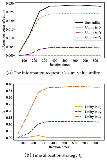
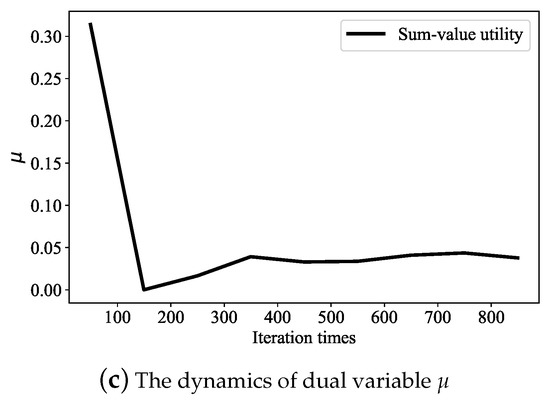
Figure 8.
Convergence of the gradient-based solution for aged utility maximization in spatial-temporal crowdsensing.
Figure 8a shows the evolution of the sum-value utility in the iterative process. The x-coordinate denotes the time steps in iteration. We also plot the sum-value utility obtained in each time slot. The overall sum-value utility is the superposition of the utilities in all time slots. This allows us to examine the contribution of different time slots. We can observe that the sum-value utility converges to a relatively stable value after 300 iteration times. Correspondingly, the time slot in each time slot and the dual variable also converge, as shown in Figure 8b,c, respectively. At the convergence, the stochastic gradient for each time slot is close to zero. This result verifies the conclusion in Proposition 7 that the gradients for all time slots are identical to some constant. When the condition in Proposition 7 holds, there is no need to further improve the overall utility by adjusting the size of the different time slots. At the convergence, the dual multiplier approaches zero, as shown in Figure 8c. Once the sum of all time allocations becomes greater than the limit T, the value of will start to increase. This acts as the penalty term to the sum-value utility, ensuring a feasible time allocation strategy at the convergence. In Figure 9, we compare the evolution of sum-value utility with that of the max- and the min-value utilities. We observe that at the convergence the sum-value utility achieves a higher value than the other two cases, which corroborates the observation in Figure 4.
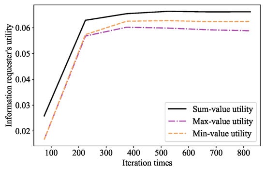
Figure 9.
Comparison of sum-, max-, and min-value utilities.
In Figure 10, we compare the sum-value utility with different prices paid to the crowd workers. The convergence to the stable value is assured for different prices. Correspondingly, Figure 11 shows the dynamics of time allocation with different prices. When we set the constant price to , we can see that gradually decreases and approaches 0 at the convergence, as shown in Figure 11a. Conversely, the time allocation and slowly grows up and reaches its maximum as the number of iterations increases. However, we will have very different observations when we set a larger price to . As shown in Figure 10b, the overall sum-value utility is dominated by the last time slot , while the sum-value utilities accumulated in and become insignificant. Correspondingly, the time allocations in and are neglectable, as shown in Figure 11b. We can see that the adjustment of the crowd workers’ unit price affects the information requester’s optimal time allocation strategy. Our algorithm proposed in this paper can dynamically adjust the time allocation strategy according to different prices so that the utility can converge to its maximum value.
Figure 10.
Sum-value utilities with different prices to crowd workers.
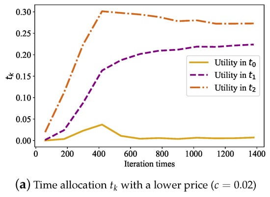
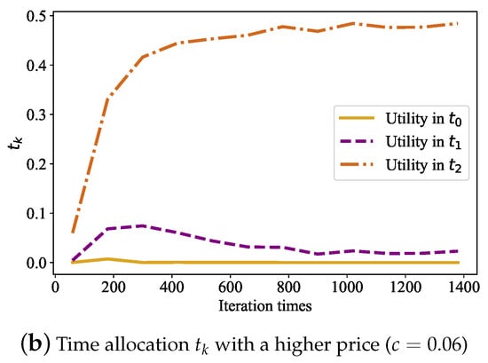
Figure 11.
Time allocation with different prices to crowd workers.
7. Conclusions
In this paper, we study a spatial-temporal crowdsourcing system consisting of a mobile access point (MAP) and a series of wireless sensor nodes. The goal is to optimize the utility of the information requester. Due to the effects of age-of-information, a series of decisions need to be made at each time slot. We, firstly, solved the optimal recruitment time slot by a gradient-based method and then obtains the optimal recruitment range. Simulation results show that our proposed method can obtain the optimal recruitment range and dynamically adjust the recruiting time according to different trade-off parameters, thereby converging to the optimal utility value.
Author Contributions
Conceptualization, X.L.; Methodology, J.X.; Project administration, C.L.; Software, C.C.; Supervision, J.X.; Validation, C.C.; Writing—original draft, X.L.; Writing—review & editing, W.Z. and C.Z. All authors have read and agreed to the published version of the manuscript.
Funding
This research was funded by China Three Gorges Corporation.
Conflicts of Interest
The authors declare no conflict of interest.
Appendix A
Appendix A.1. Proof for Proposition 1
With the sum-value utility, the information requester’s payoff term is strictly decreasing with respect to (w.r.t.) the recruiting range D, while the second cost term is linearly increasing w.r.t. D. The first- and second-order derivatives of the sum-value utility is given as follows:
Let , we have , and let we have , which implies the solution where denotes the Lambert W function. The results in Proposition 1 follow the discussion over two cases. When , we have and, thus, . The optimal to (5) is taken at the stationary point . When or , we find that and moreover is concave in and convex in . Note that is decreasing in and increasing in , the optimal in this case is achieved also at .
Appendix A.2. Proof for Proposition 2
Given the recruiting parameters , the maximum value of the Poisson point process is a random variable. Hence, we first evaluate the cumulative distribution function (CDF) for the maximum value M and than calculate the expected max-value payoff function by the integration . Let denote the number of active sensors in the circular region with radius D and denote the CDF of the random variable M, then we have the following equations:
The last equality is due to the fact the crowd worker is uniformly distributed in the circular region with the radius D. Let for notational simplicity. Thus, the sum-value payoff function can be simplified as follows:
The second equation in (A3) relies on the following property:
By a change of variable, i.e., , we have , and then the sum-value payoff can be rewritten in a compact form as follows:
Inserting time span T in (A4), we can obtain the equation in (13).
The evaluation of the min-value payoff follows a similar approach as that for the max-value payoff . Let , then we have
Similarly define , the min-value payoff function can be simplified as follows:
Inserting time span T in (A5), we can obtain the equation in (14).
References
- Li, G.; Wang, J.; Zheng, Y.; Franklin, M.J. Crowdsourced data management: A survey. IEEE Trans. Knowl. Data Eng. 2016, 28, 2296–2319. [Google Scholar] [CrossRef]
- Tong, Y.; Zhou, Z.; Zeng, Y.; Chen, L.; Shahabi, C. Spatial crowdsourcing: A survey. VLDB J. 2020, 29, 217–250. [Google Scholar] [CrossRef]
- Qiu, J.; Tian, Z.; Du, C.; Zuo, Q.; Su, S.; Fang, B. A survey on access control in the age of internet of things. IEEE Internet Things J. 2020, 7, 4682–4696. [Google Scholar] [CrossRef]
- Restuccia, F.; Ghosh, N.; Bhattacharjee, S.; Das, S.K.; Melodia, T. Quality of Information in Mobile Crowdsensing: Survey and Research Challenges. ACM Trans. Sens. Netw. 2017, 13, 1–43. [Google Scholar] [CrossRef]
- Jiang, W.; Han, B.; Habibi, M.A.; Schotten, H.D. The Road Towards 6G: A Comprehensive Survey. IEEE Open J. Commun. Soc. 2021, 2, 334–366. [Google Scholar] [CrossRef]
- Wang, Z.; Hu, J.; Wang, Q.; Lv, R.; Wei, J.; Chen, H.; Niu, X. Task-bundling-based incentive for location-dependent mobile crowdsourcing. IEEE Commun. Mag. 2019, 57, 54–59. [Google Scholar] [CrossRef]
- Zhang, J.; Wang, Z.; Wang, D.; Zhang, X.; Gupta, B.; Liu, X.; Ma, J. A Secure Decentralized Spatial Crowdsourcing Scheme for 6G-Enabled Network in Box. IEEE Trans. Ind. Inform. 2021, 18, 6160–6170. [Google Scholar] [CrossRef]
- Micholia, P.; Karaliopoulos, M.; Koutsopoulos, I.; Aiello, L.M.; Morales, G.D.F.; Quercia, D. Incentivizing social media users for mobile crowdsourcing. Int. J. Hum.-Comput. Stud. 2017, 102, 4–13. [Google Scholar] [CrossRef]
- Guo, B.; Chen, H.; Nan, W.; Yu, Z.; Xie, X.; Zhang, D.; Zhou, X. TaskMe: Toward a dynamic and quality-enhanced incentive mechanism for mobile crowd sensing. Int. J. Hum.-Comput. Stud. 2017, 102, 14–26. [Google Scholar] [CrossRef]
- Wu, P.; Ngai, E.W.; Wu, Y. Toward a real-time and budget-aware task package allocation in spatial crowdsourcing. Decis. Support Syst. 2018, 110, 107–117. [Google Scholar] [CrossRef]
- Huang, Y.; White, C.; Xia, H.; Wang, Y. A computational cognitive modeling approach to understand and design mobile crowdsourcing for campus safety reporting. Int. J. Hum.-Comput. Stud. 2017, 102, 27–40. [Google Scholar] [CrossRef]
- Zhao, P.; Li, X.; Gao, S.; Wei, X. Cooperative task assignment in spatial crowdsourcing via multi-agent deep reinforcement learning. J. Syst. Archit. 2022, 128, 102551. [Google Scholar] [CrossRef]
- Ma, F.; Liu, X.; Liu, A.; Zhao, M.; Wang, T. A Time and Location Correlation Incentive Scheme for Deep Data Gathering in Crowdsourcing Networks. Wirel. Commun. Mob. Comput. 2018, 2018, 1–22. [Google Scholar] [CrossRef]
- Song, T.; Xu, K.; Li, J.; Li, Y.; Tong, Y. Multi-skill aware task assignment in real-time spatial crowdsourcing. GeoInformatica 2020, 24, 153–173. [Google Scholar] [CrossRef]
- Cheng, P.; Lian, X.; Chen, Z.; Fu, R.; Chen, L.; Han, J.; Zhao, J. Reliable Diversity-Based Spatial Crowdsourcing by Moving Workers. Proc. VLDB Endow. 2015, 8, 1022–1033. [Google Scholar] [CrossRef]
- Zhai, D.; Liu, A.; Chen, S.; Li, Z.; Zhang, X. SeqST-ResNet: A sequential spatial temporal ResNet for task prediction in spatial crowdsourcing. In Proceedings of the International Conference on Database Systems for Advanced Applications, Chiang Mai, Thailand, 22–25 April 2019; pp. 260–275. [Google Scholar]
- Muhammad, A.; Elhattab, M.; Arfaoui, M.A.; Al-Hilo, A.; Assi, C. Age of Information Optimization in a RIS-Assisted Wireless Network. arXiv 2021, arXiv:2103.06405. [Google Scholar]
- Kadota, I.; Modiano, E. Minimizing the age of information in wireless networks with stochastic arrivals. IEEE Trans. Mob. Comput. 2019, 20, 1173–1185. [Google Scholar] [CrossRef]
- Kadota, I.; Sinha, A.; Modiano, E. Optimizing Age of Information in Wireless Networks with Throughput Constraints. In Proceedings of the IEEE INFOCOM 2018—IEEE Conference on Computer Communications, Honolulu, HI, USA, 16–19 April 2018; pp. 1844–1852. [Google Scholar] [CrossRef]
- Abd-Elmagid, M.A.; Pappas, N.; Dhillon, H.S. On the Role of Age of Information in the Internet of Things. IEEE Commun. Mag. 2019, 57, 72–77. [Google Scholar] [CrossRef]
- Yates, R.D.; Sun, Y.; Brown, D.R.; Kaul, S.K.; Modiano, E.; Ulukus, S. Age of information: An introduction and survey. IEEE J. Sel. Areas Commun. 2021, 39, 1183–1210. [Google Scholar] [CrossRef]
- Mankar, P.D.; Abd-Elmagid, M.A.; Dhillon, H.S. Spatial distribution of the mean peak age of information in wireless networks. IEEE Trans. Wirel. Commun. 2021, 20, 4465–4479. [Google Scholar] [CrossRef]
- Katsidimas, I.; Nikoletseas, S.; Raptopoulos, C. Power efficient algorithms for wireless charging under phase shift in the vector model. In Proceedings of the 2019 15th International Conference on Distributed Computing in Sensor Systems (DCOSS), Santorini Island, Greece, 29–31 May 2019; pp. 131–138. [Google Scholar]
- López, O.L.; Alves, H.; Souza, R.D.; Montejo-Sánchez, S.; Fernández, E.M.G.; Latva-Aho, M. Massive wireless energy transfer: Enabling sustainable IoT toward 6G era. IEEE Internet Things J. 2021, 8, 8816–8835. [Google Scholar] [CrossRef]
- Mukase, S.; Xia, K.; Umar, A.; Owoola, E.O. On-Demand Charging Management Model and Its Optimization for Wireless Renewable Sensor Networks. Sensors 2022, 22, 384. [Google Scholar] [CrossRef] [PubMed]
- Dudak, J.; Gaspar, G.; Sedivy, S.; Fabo, P.; Pepucha, L.; Tanuska, P. Serial communication protocol with enhanced properties–securing communication layer for smart sensors applications. IEEE Sens. J. 2018, 19, 378–390. [Google Scholar] [CrossRef]
- Zou, J.; Ye, B.; Qu, L.; Wang, Y.; Orgun, M.; Li, L. A proof-of-trust consensus protocol for enhancing accountability in crowdsourcing services. IEEE Trans. Serv. Comput. 2018, 12, 429–445. [Google Scholar] [CrossRef]
- Zhang, Y.J.A.; Qian, L.; Huang, J. Monotonic Optimization in Communication and Networking Systems. Found. Trends Netw. 2013, 7, 1–75. [Google Scholar] [CrossRef]
- Feijer, D.; Paganini, F. Stability of primal–dual gradient dynamics and applications to network optimization. Automatica 2010, 46, 1974–1981. [Google Scholar] [CrossRef]
- Boyd, S.; Vandenberghe, L. Convex Optimization; Cambridge University Press: Cambridge, UK, 2004. [Google Scholar]


Publisher’s Note: MDPI stays neutral with regard to jurisdictional claims in published maps and institutional affiliations. |
© 2022 by the authors. Licensee MDPI, Basel, Switzerland. This article is an open access article distributed under the terms and conditions of the Creative Commons Attribution (CC BY) license (https://creativecommons.org/licenses/by/4.0/).