Software in-the-Loop Simulation of an Advanced SVM Technique for 2ϕ-Inverter Control Fed a TPIM as Wind Turbine Emulator

Abstract

An appropriate modulation scheme selection ensures inverter performance. Thus, space vector modulation (SVM) is more efficient and has its own distinct advantages compared to other pulse width modulation (PWM) techniques. This work deals with the development of an advanced space vector pulse width modulation (SVM) technique for two-phase inverter control using an XSG library to ensure rapid prototyping of the controller FPGA implementation. The proposed architecture is applied digitally and in real time to drive a two-phase induction motor (TPIM) for small-scale wind turbine emulation (WTE) profiles in laboratories with minimum current ripple and torque oscillation. Four space voltage vectors generated for the used SVM technique do not contain a zero vector. Hence, for an adequate adjustment of these four vectors, a reference voltage vector located in the square locus is determined. Considering the asymmetry between the main and auxiliary windings, the TPIM behavior, which is fed through the advanced SVM controlled-two-phase inverter (2ϕ-inverter), is studied, allowing us to control the speed and the torque under different conditions for wind turbine emulation. Several quantities, such as electromagnetic torque, rotor fluxes, stator currents and speed, are analyzed. To validate the obtained results using both Simulink and XSG interfaces, the static and dynamic characteristics of the WTE are satisfactorily reproduced. The collected speed and torque errors between the reference and actual waveforms show low rates, proving emulator controller effectiveness.

1. Introduction

Electrical power systems based on renewable energy sources are dominated by power electronic converters and electrical machines, which are deployed for the integration of renewable power plants, responsive demand and different storage systems types [1,2,3]. The stability of these systems requires a robust control strategy applied to the power converters [4]. Therefore, laboratory-scale setups are becoming the key tools for prototyping and evaluating the performance and robustness of different system parts from the renewable source extraction to the system grid connection [5,6].

Among the renewable sources, recently, there has been a considerable amount of growth in the wind energy system field due to various technological advancements, since wind energy’s efficiency depends directly on wind speed and frequency [7]. The wind’s renewable nature and abundance make it a good candidate for providing energy on a large scale, although it is difficult to accurately predict it because of the many factors on which it depends. Hence, aerodynamic study for wind power capture [8], electric generators and power converters design [9,10,11], system control and energy generation optimization [12,13,14] are just a few examples of the challenges that still face engineers and researchers.

Testing wind energy conversion systems under real operating conditions is unfordable for small wind generator manufacturers or academic researchers due to the magnitude of these installations and their costs [15,16]. A more economically viable solution is to implement a wind turbine emulation system. In a wind emulator, the turbine is replaced by an electromechanical actuator that is mechanically coupled to the electrical generator, which incorporates the wind profile model as a reference speed into the control board.

Some implementations of WTE have been developed in literature [17,18,19,20,21,22,23,24]. WTE’s design can involve the use of different types of electrical motors such as DCM and PMSM [25,26,27,28]. DCM, used in [29], is the most commonly considered due to its design simplicity, easy torque or speed control through the armature current and cost-effectiveness, since it needs a simple buck converter control structure. However, this machine requires permanent maintenance. Moreover, the squirrel cage induction motor (SCIM) [30] and the doubly fed induction motor (DFIM) [31] are also used for wind turbine emulation study.

Numerous control strategies have been applied for WTE design. In case of DCM, PI controllers are the most basic and highly used approach [32]. Otherwise, for the induction motor (IM), field-oriented control is considered [29,30]. Generally, these motors are fed through power converters which perform as variable-speed drives for both AC and DC modes. Hence, their control techniques are included in the WTE study to generate the appropriate pulse signals for each corresponding case, namely, a chopper or an inverter [33].

For the purposes of AC motors drives, the conventional sinusoidal pulse width modulation (SPWM) control technique has been replaced by the SVM control technique due to its switching losses reduction and its key characteristics, such as better DC voltage utilization and easiness for digital implementation [34]. Moreover, it offers better output voltage and current qualities in order to improve inverter performance whatever the topology, such as two-level, three-level and five-level inverters [35]. Therefore, the switching states and triangle numbers become quite large, which causes complexities in on-time computations of switching periods by increasing the inverter level. Hence, the conventional SVM algorithms become impractical as the inverter’s level increases. So far, numerous SVM algorithms have been presented in literature [36] to mitigate the problem associated with computational complexities which are considered an industrial standard for AC drives, since the multilevel inverter is widely used in transportation and industrial automation [37] for three-phase AC motors or servo systems vector control [38] but is weakly used for two-phase AC motor drives.

The two-phase induction motors, known as single-phase induction motors (SPIM), are used extensively in low- or middle-power level fields, especially in households, because a three-phase supply is not required [39]. Most of the equipment operates at constant speed and with a certain inertia due to the load applied to the rotor. Although they are simpler than three-phase induction motors and have lower production costs, two-phase AC motors analysis is more complex. The operating principle of these machine types is based on capacitor use to create starting torque through auxiliary winding. Accordingly, they operate as asymmetrical two-phase induction motors at the start but as pure single-phase induction motors while running after a centrifugal switch is opened. Taking into account the asymmetry between the TPIM main and auxiliary stator windings, a consolidated study and a computational model are required to calculate the motor parameters under load variations and to make it suitable for adjustable speed control.

In this paper, the advanced SVM technique for the two-phase inverter-fed symmetrical induction motor for a laboratory-scale wind turbine emulation is proposed. The controller is designed through both Simulink and XSG interfaces for allowing software in-the-loop simulation and real-time visualization of the WTE characteristics under different operation modes. The main technical contributions compared to others’ configurations are summarized in

Table 1. Brief review of different WTE configurations and control.

Ref.	Prime Motor	Converter Type	Controller Use	Observer Use	Supports	Required Measurements Type and Number
[40]	DCM	Thyristorized bidirectional rectifier	Required (PI controller)	No observer used	DSP	Current Torque Speed
[24]	DCM	DC/DC converter	Required (PI controller)	No observer used	dSPACE	Speed Current
[32]	DCM	DC/DC buck converter	Required (PI controller)	No observer used	FPGA	Speed Current
[41]	DCM	DC/DC boost converter	Not required	Required (STA-SMO observer)	dSPACE	Voltage Current
[42]	PMSM	Three-phase IGBT inverter	Required (PI controller)	No observer used	dSPACE	Position Two current
[22]	SCIM	Three-phase IGBT inverter	Required (PI controller)	No observer used	Intel 80C196KD µc	Torque Speed
This work	2ϕIM	Two-phase IGBT inverter	Required (PI controller)	No observer used	FPGA	Speed Two current

. This brief review is carried out based on six criteria, namely, the prime motor type; the associated converter topology; the control algorithm technique, if there is one; the use of an observer or the lack thereof; the digital platform for hardware implementation and the required type and number of measured parameters.

This paper is organized as follows. Section 2 describes the proposed approach for the advanced SVM technique development without zero space vectors. Section 3 deals with the mathematical model for the TPIM as the electromechanical actuator part of the wind turbine conversion system based on the emulator. Section 4 presents the software in-the-loop simulation results for the two-phase inverter controller associated with the WTE. A comparative study based on the recorded reference and actual speed and torque error rates is analyzed. Section 5 focuses on the XSG design of the advanced SVM technique for emulator digital controlling in real time. The obtained results are also discussed. Section 6 summarizes the most important points of the proposals developed in this paper.

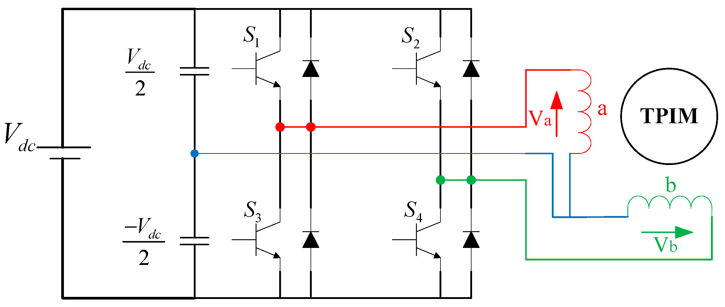
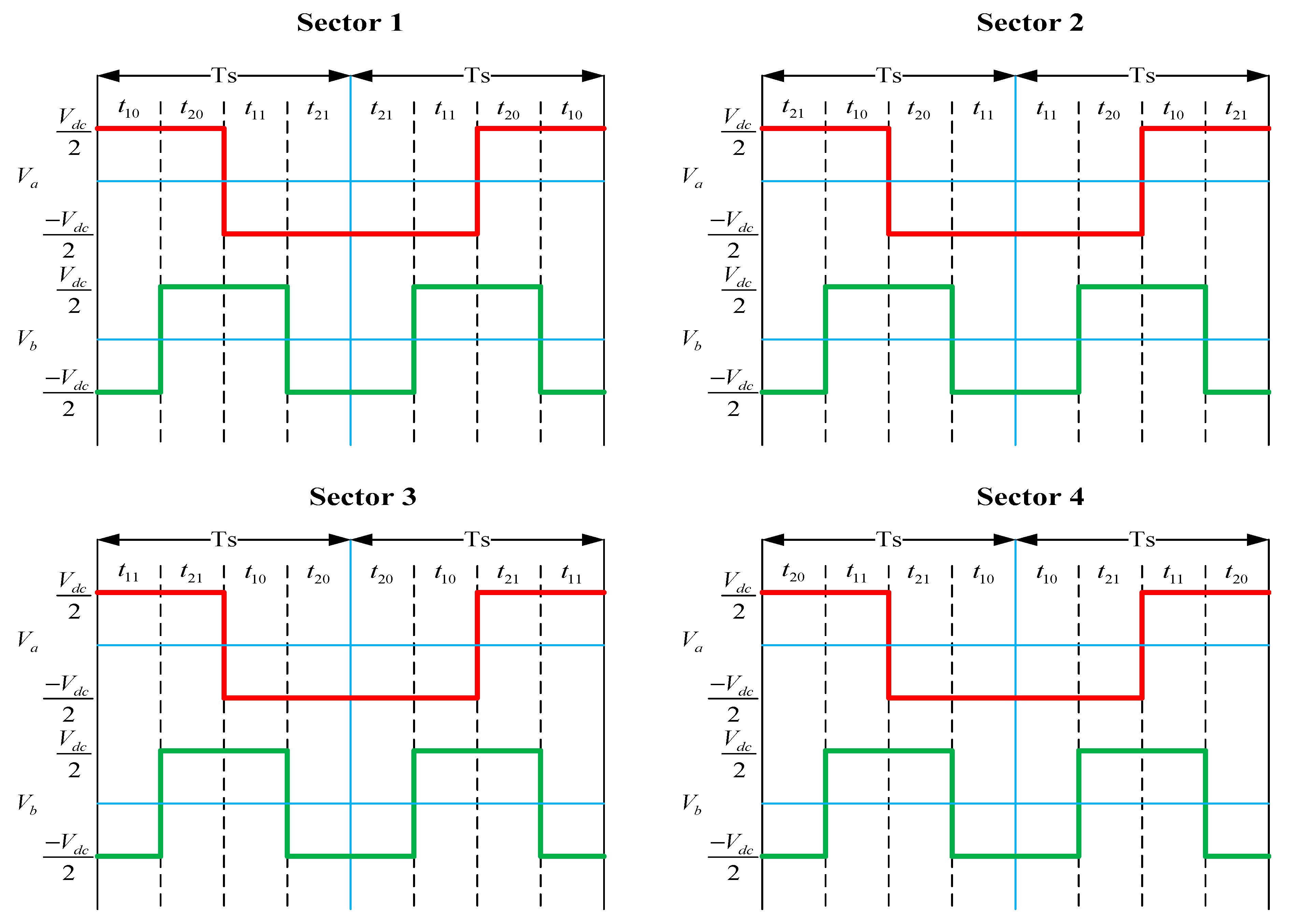
2. Advanced Four Space Vectors Modulations Technique for 2ϕ-Inverter

Instead of the single-phase induction motor, the two-phase induction motor is chosen in this study as the model motor. It operates without negative torque and maintains high efficiency by supplying the balanced voltage source without harmonics to the symmetrical two-phase induction motor [43].

The typical structure of the two-phase half-bridge inverter for the two-phase induction motors is depicted in Figure 1.

The output voltages V_a and V_b of windings a and b, respectively, are expressed in the balanced equation system as:

$$\{\begin{array}{l}{V}_a=\frac{V_{dc}}{2}{m}_{}^{}\sin \omega t\\ V_b=\frac{V_{dc}}{2}{m}_{}^{}\sin (\omega t-\frac{\pi }{2})\end{array}$$

(1)

where m is the modulation index.

As shown in Figure 2, four switching states are formed in the two-phase inverter when four switches are adjusted. The four space voltage vectors originate based on the possible combinations of four individual switches signified by switching states labeled as [S₁, S₂, S₃, S₄].

Four space vectors, which are uniformly distributed at $\frac{\pi }{2}$ with a length of $\frac{Vdc}{\sqrt{2}}$, form an exact square in two-phase inverters, but zero vectors are not included, as presented in Figure 3. ‘0’ denotes connection to the negative dc link and ‘1’ denotes connection to the positive dc link.

The complex representation of the four space voltage vectors is expressed as:

$${\overrightarrow{V}}_k=\frac{1}{\sqrt{2}}{V}_{dc}{}_{}^{}{e}^{j(k-1)\frac{\pi }{2}}$$

(2)

where k = 1, 2, 3, 4.

The advanced SVM technique proposed in this section does not use zero vectors. Hence, an appropriate exploitation of each sector’s vectors, which are used to locate the reference vector, is strongly requested. The time duration for the reference vector V_ref is determined by adjusting four voltage space vectors. Figure 4 illustrates the model sectors where the reference vector is located in all sectors.

The sectors are divided into two voltage space vectors which are adjacent to the V_ref in each case. Two associated time durations spent on the two voltage space vectors are used. However, the two time duration amounts do not satisfy the constant sampling interval T_s for allowing the reference vector to arrive at the maximum voltage locus. Accordingly, since there are no zero vectors, the sampling interval remainder should be spent in the main sector and the relevant diagonal sector. Considering the main sector, which is Sector 1, the time duration amount spent on the modified reference vector is defined as:

$$V_{ref}+\frac{\Delta V}{2}$$

(3)

The restraint vector in the diagonal sector ($-\frac{\mathsf{\Delta }V}{2}$) is equal to the sampling time expressed as:

$$T_s=t_{10}+t_{20}+t_{11}+t_{21}$$

(4)

where t₁₀ = t₁ + t₁₁ and t₂₀ = t₂ + t₂₁ and ΔV represents the difference vector between V_ref and the maximum voltage locus.

In the main sector, t₁ and t₂ are the time duration spent respectively on V₁ and V₂, while t₁₁ and t₂₁ are those spent on V₃ and V₄, respectively, in the corresponding diagonal sector.

At ωt = θ, the absolute value of the maximum space vector to the square locus is computed as:

$$\left|\Delta {\overrightarrow{V}}_{\max }\right|=\left|{\overrightarrow{V}}_{ref}+\Delta \overrightarrow{V}\right|=\frac{V_{dc}}{\sqrt{2}\left(\sin \theta +\cos \theta \right)}$$

(5)

where θ is the counterclockwise phase angle from V₁ to V_ref. It is between 0° and 90° in Sector 1. From (5), the difference vector, the modified reference vector and the restraint vector in the diagonal sector absolute values are given by the following equation system:

$$\{\begin{array}{l}\left|\Delta \overrightarrow{V}\right|=\frac{V_{dc}}{\sqrt{2}\left(\sin \theta +\cos \theta \right)}-\left|{\overrightarrow{V}}_{ref}\right|\\ \left|{\overrightarrow{V}}_{ref}+\frac{\Delta \overrightarrow{V}}{2}\right|=\frac{V_{dc}}{2\sqrt{2}\left(\sin \theta +\cos \theta \right)}+\left|\frac{{\overrightarrow{V}}_{ref}}{2}\right|\\ \left|\frac{-\Delta \overrightarrow{V}}{2}\right|=\frac{V_{dc}}{2\sqrt{2}\left(\sin \theta +\cos \theta \right)}-\left|\frac{{\overrightarrow{V}}_{ref}}{2}\right|\end{array}$$

(6)

Based on Figure 4, the relations between the time durations t₁₀ and t₂₀ and the modified reference vector in the main sector are expressed as:

$$\{\begin{array}{l}{T}_{s_{(V1)}}:t_{10}=\frac{V_{dc}}{\sqrt{2}}:\left|V_{ref}+\frac{\Delta V}{2}\right|\cos \theta \\ T_{s_{(V2)}}:t_{20}=\frac{V_{dc}}{\sqrt{2}}:\left|V_{ref}+\frac{\Delta V}{2}\right|\sin \theta \end{array}$$

(7)

Similarly, the time durations t₁₁ and t₂₁ and the restraint reference vector in the diagonal sector are related by:

$$\{\begin{array}{l}{T}_{s_{(V3)}}:t_{11}=\frac{V_{dc}}{\sqrt{2}}:\left|-\frac{\Delta V}{2}\right|\cos \theta \\ T_{s_{(V4)}}:t_{21}=\frac{V_{dc}}{\sqrt{2}}:\left|-\frac{\Delta V}{2}\right|\sin \theta \end{array}$$

(8)

By substituting Equation (6) in Equation (7) and Equation (8) respectively, the time durations t₁, t₂, t₃ and t₄ are solved as:

$$\{\begin{array}{l}{t}_{10}=\frac{\sqrt{2}{T}_s}{V_{dc}}\left[\frac{V_{dc}}{2\sqrt{2}\left(\sin \theta +\cos \theta \right)}+\left|\frac{{\overrightarrow{V}}_{ref}}{2}\right|\right]\cos \theta \\ t_{20}=\frac{\sqrt{2}{T}_s}{V_{dc}}\left[\frac{V_{dc}}{2\sqrt{2}\left(\sin \theta +\cos \theta \right)}+\left|\frac{{\overrightarrow{V}}_{ref}}{2}\right|\right]\sin \theta \\ t_{11}=\frac{\sqrt{2}{T}_s}{V_{dc}}\left[\frac{V_{dc}}{2\sqrt{2}\left(\sin \theta +\cos \theta \right)}-\left|\frac{{\overrightarrow{V}}_{ref}}{2}\right|\right]\cos \theta \\ t_{21}=\frac{\sqrt{2}{T}_s}{V_{dc}}\left[\frac{V_{dc}}{2\sqrt{2}\left(\sin \theta +\cos \theta \right)}-\left|\frac{{\overrightarrow{V}}_{ref}}{2}\right|\right]\sin \theta \end{array}$$

(9)

In order to determine all the duty cycles d₁, d₂, d₃ and d₄, the time durations should be divided by T_s as follows:

$$\{\begin{array}{l}{d}_1=\frac{t_{10}}{T_s}=\frac{\sqrt{2}}{V_{dc}}\left[\frac{V_{dc}}{2\sqrt{2}\left(\sin \theta +\cos \theta \right)}+\left|\frac{{\overrightarrow{V}}_{ref}}{2}\right|\right]\cos \theta \\ d_2=\frac{t_{11}}{T_s}=\frac{\sqrt{2}}{V_{dc}}\left[\frac{V_{dc}}{2\sqrt{2}\left(\sin \theta +\cos \theta \right)}+\left|\frac{{\overrightarrow{V}}_{ref}}{2}\right|\right]\sin \theta \\ d_3=\frac{t_{20}}{T_s}=\frac{\sqrt{2}}{V_{dc}}\left[\frac{V_{dc}}{2\sqrt{2}\left(\sin \theta +\cos \theta \right)}-\left|\frac{{\overrightarrow{V}}_{ref}}{2}\right|\right]\cos \theta \\ d_4=\frac{t_{21}}{T_s}=\frac{\sqrt{2}}{V_{dc}}\left[\frac{V_{dc}}{2\sqrt{2}\left(\sin \theta +\cos \theta \right)}-\left|\frac{{\overrightarrow{V}}_{ref}}{2}\right|\right]\sin \theta \end{array}$$

(10)

The last step consists of determining the switching sequence by the two-phase symmetrical modulation of the 2ϕ SVM when the main sector changes. When the reference vector sweeps any sector, the switching sequence is considered to make the suitable PWM waveform in the 2ϕ-inverter. In order to realize the reference vector, the four space vectors as well as the four time durations should be determined and adjusted by four switches during T_s. The switching sequence is expressed as:

$${\overline{V}}_{ref}{T}_s={\overline{V}}_1{t}_{10}+{\overline{V}}_2{t}_{20}+{\overline{V}}_3{t}_{11}+{\overline{V}}_4{t}_{21}$$

(11)

Hence, four sets of output voltages V_a and V_b are generated, as presented in Figure 5.

In the main sector, the reference vector begins at V₁ and finishes at V₄ in the diagonal sector with the time durations t₁₀ and t_21, respectively. This rule is applied on all sectors because the main vector can begin at another space vector such as V₂, V₃ or V₄, reserving the symmetry during 2T_s. From Figure 5, it is noted that two inverter legs carry out either one switching for V_a or two switching for V_b regularly during 2T_s to determine the suitable PWM output voltages. For the conventional SVM technique, these waveforms are difficult to implement on hardware platforms because, according to the sector number, the switching operations during 2T_s are changed irregularly, as illustrated in Figure 6.

This leads to switching loss increase because the output voltage is discontinuous at the sector boundary. In addition, the significant surge is involved in the output current and therefore the ripples are significant. In order to eliminate the previously mentioned 2ϕ symmetrical modulation disadvantages, the advanced technique is applied in switching operations, ensuring that the output voltage becomes continuous at the boundary between sectors. In this case, the PWM voltage waveforms are uniform and easy to implement because the switching logic is regular. Hence, during T_s, the inverter leg of phase A is carried out with one switching at t = t_A, while that of phase B proceeds with two switching, namely at t = t_B1 and t = t_B2, based on the specific calculating method, as summarized in

Table 2. Switching arrangement for the advanced SVM symmetrical modulation realization.

	State	Time Switching during 2 × Ts
		t10	t20	t11	t21	t10	t20	t11	t21
Sector 1	tA	1	1	0	0	0	0	1	1
	tB1	1	0	0	0	0	0	0	1
	tB2	1	1	1	0	0	1	1	1
Sector 2	tA	1	0	0	1	0	1	1	0
	tB1	0	0	0	1	0	0	1	0
	tB2	1	1	0	1	1	1	1	0
Sector 3	tA	0	0	1	1	1	1	0	0
	tB1	0	0	1	0	0	1	0	0
	tB2	1	0	1	1	1	1	0	1
Sector 4	tA	0	1	1	0	1	0	0	1
	tB1	0	1	0	0	1	0	0	0
	tB2	0	1	1	1	1	0	1	1

.

3. Mathematical Model of the Proposed Wind Turbine Emulator

A fundamental aspect of WTE building is to acknowledge the relationship between the wind turbine mechanical torque or rotational speed and the power output with the physical quantities such as air density, wind speed profile, rotor swept area, etc. The basic study proposed in this paper consists of emulating the wind profile through a two-phase induction motor by introducing the wind turbine speed in the machine model as the reference speed.

3.1. Mathematical Model of the Proposed Wind Turbine Emulator

The TPIM equivalent circuit in terms of stationary frame, represented by the q-axis for the main winding and d-axis for auxiliary winding, is illustrated by Figure 7.

Considering that core saturation and iron losses are neglected, the mathematical model of the two-phase induction motor in the d–q stationary reference frame, which defines its dynamic behavior, is represented by some equations. Equation (12) represents the d–q axes’ stator and rotor voltages.

$$\{\begin{array}{l}{v}_{sd}^s=r_{sd}{i}_{sd}^s+\frac{d{\varphi }_{sd}^s}{dt}\\ v_{sq}^s=r_{sq}{i}_{sq}^s+\frac{d{\varphi }_{sq}^s}{dt}\\ 0=r_r{i}_{rd}^s+\frac{d{\varphi }_{rd}^s}{dt}+{\omega }_r{\varphi }_{rq}^s\\ 0=r_r{i}_{rq}^s+\frac{d{\varphi }_{rq}^s}{dt}-{\omega }_r{\varphi }_{rd}^s\end{array}$$

(12)

Equation (13) depicts the d–q axes’ stator and rotor fluxes.

$$\{\begin{array}{l}{\varphi }_{sd}^s=l_{sd}{i}_{sd}^s+m_{srd}{i}_{rd}^s\\ {\varphi }_{sq}^s=l_{sq}{i}_{sq}^s+m_{srq}{i}_{rq}^s\\ {\varphi }_{rd}^s=l_r{i}_{rd}^s+m_{srd}{i}_{sd}^s\\ {\varphi }_{rq}^s=l_r{i}_{rq}^s+m_{srq}{i}_{sq}^s\end{array}$$

(13)

The electromagnetic torque and mechanical equation are given respectively by Equations (14) and (15).

$$T_e=P\left(m_{srq}{i}_{sq}^s{i}_{rd}^s-m_{srd}{i}_{sd}^s{i}_{rq}^s\right)$$

(14)

$$P\left(T_e-T_L\right)=J\frac{d{\omega }_r}{dt}+f{\omega }_r$$

(15)

According to Equation (15), it is noted that the asymmetry appears in the model due to unequal main and auxiliary stator windings resistances and inductances. Hence, this asymmetry can be eliminated by using an appropriate variable changing as follows:

$$\{\begin{array}{l}{i}_{sd}^s=i_{s{d}^{’}}^s\\ i_{sq}^s=A\times i_{s{q}^{*}}^s\end{array}$$

(16)

where

$$A=\frac{m_{srd}}{m_{srq}}$$

(17)

This assumption allows us to reduce the torque oscillation of the symmetrical TPIM model. Hence, by substituting the variables $i_{sd}^s$ and $i_{sq}^s$ for $i_{s{d}^{*}}^s$ and $i_{s{q}^{*}}^s$ into Equation (14), the torque expression is rewritten as:

$$T_e=\frac{P}{l_r}{m}_{srd}\left(i_{sq*}^s{\varphi }_{rd}^s-i_{sd*}^s{\varphi }_{rq}^s\right)$$

(18)

The symmetrical state model of the TPIM in the stationary reference frame is written in the following form:

$$\frac{d\left[X\right]}{dt}=\left[A\right]\left[X\right]+\left[B\right]\left[U\right]$$

(19)

where $\left[X\right],\left[U\right],\left[A\right]\mathrm{and}\left[B\right]$ are respectively the state vector, the control vector, the state matrix and the control matrix, defined as follows:

$$\left[X\right]={\left[i_{sd*}^s{}_{}^{}{i}_{sq*}^s{}_{}^{}{\varphi }_{rd*}^s{}_{}^{}{\varphi }_{rq*}^s{}_{}^{}{\omega }_r\right]}^T$$

(20)

$$\left[U\right]={\left[v_{sd*}^s{}_{}^{}{v}_{sq*}^s{}_{}^{}{T}_L\right]}^T$$

(21)

$$\left[A\right]=\left[\begin{array}{ccccc}-\frac{1}{{\sigma }_d{\tau }_{sd}}-\frac{1-{\sigma }_d}{{\sigma }_d{\tau }_r}& 0& \frac{1-{\sigma }_d}{{\sigma }_d{m}_{srd}{\tau }_r}& \frac{1-{\sigma }_d}{{\sigma }_d{m}_{srd}}{\omega }_r& 0\\ 0& -\frac{A^2{r}_{sq}}{r_{sd}{\sigma }_d{\tau }_{sd}}-\frac{1-{\sigma }_d}{{\sigma }_d{\tau }_r}& -\frac{1-{\sigma }_d}{{\sigma }_d{m}_{srd}}{\omega }_r& \frac{1-{\sigma }_d}{{\sigma }_d{m}_{srd}{\tau }_r}& 0\\ \frac{m_{srd}}{{\tau }_r}& 0& -\frac{1}{{\tau }_r}& {\omega }_g& 0\\ 0& \frac{m_{srd}}{{\tau }_r}& -{\omega }_g& -\frac{1}{{\tau }_r}& 0\\ -\frac{P^2{m}_{srd}}{J{l}_r}{\varphi }_{rq}^s& \frac{P^2{m}_{srd}}{J{l}_r}{\varphi }_{rd}^s& 0& 0& -\frac{f}{J}\end{array}\right]$$

(22)

$$\left[B\right]=\left[\begin{array}{ccc}\frac{1}{{\sigma }_d{l}_{sd}}& 0& 0\\ 0& \frac{1}{{\sigma }_q{l}_{sq}}& 0\\ 0& 0& 0\\ 0& 0& 0\\ 0& 0& -\frac{P}{J}\end{array}\right]$$

(23)

In which,

$$\{\begin{array}{l}{\tau }_{sd}=\frac{l_{sd}}{r_{sd}}\\ {\tau }_{sq}=\frac{l_{sq}}{r_{sq}}\\ {\tau }_r=\frac{l_r}{r_r}\\ {\sigma }_d=1-\frac{m_{{}_{srd}}^2}{l_{sd}{l}_r}\\ {\sigma }_q=1-\frac{m_{{}_{srq}}^2}{l_{sq}{l}_r}\end{array}$$

(24)

These parameters represent the stator time constant according the d–q axes, the rotor time constant and the Blondel dispersion coefficients according to the d–q axes, respectively.

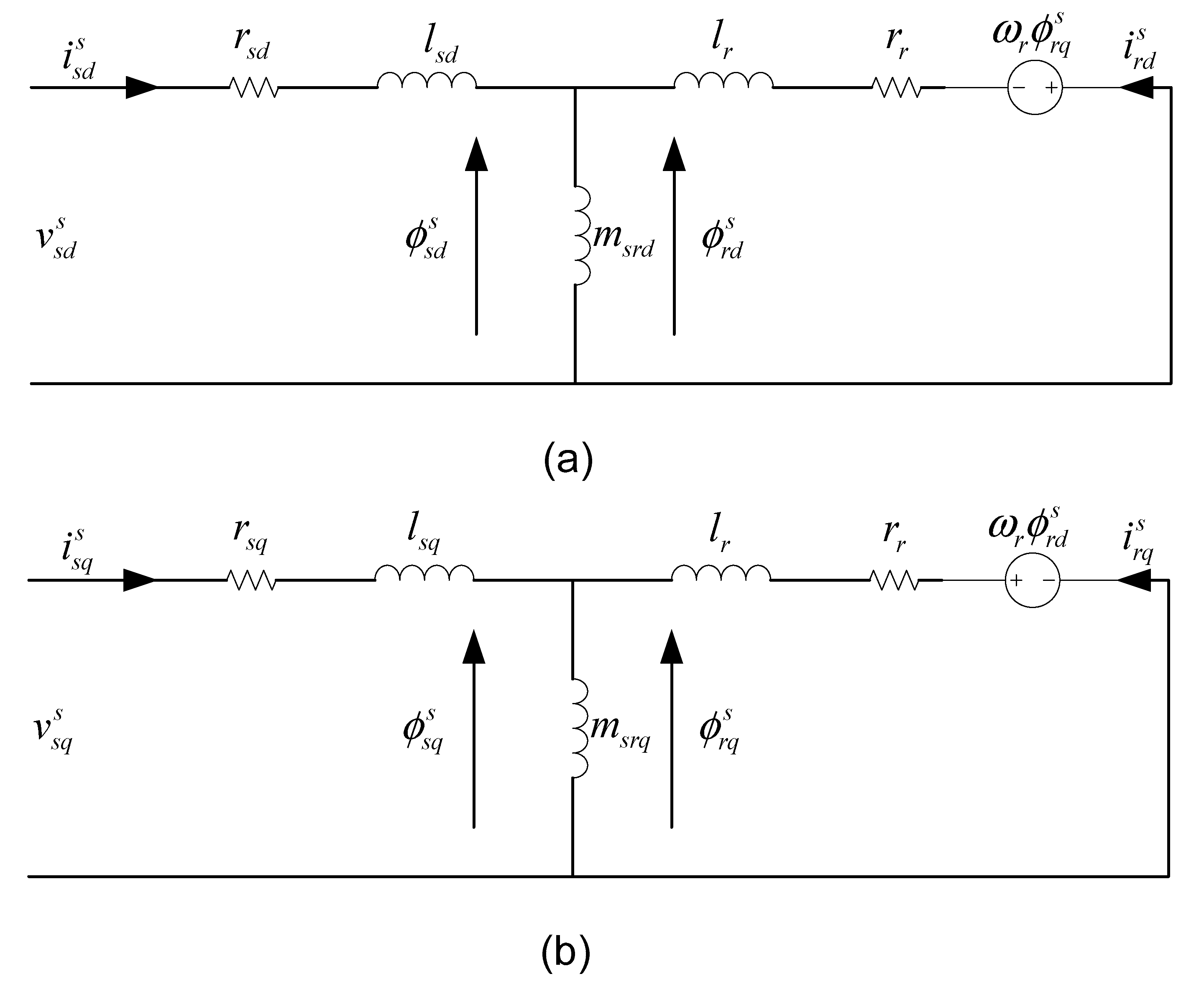
3.2. IRFOC for Symmetrical TPIM Operation

The indirect rotor field-oriented control method for symmetrical TPIM is derived from vector-controlled three phase AC electrical machine. It consists on directing the currents supplied to the machine in phase and quadrature for the rotor flux which leads to choose entirely with the rotor flux in d-axis as:

$$\{\begin{array}{l}{\varphi }_{rq}^{rf}=0\\ {\varphi }_{rd}^{rf}={\varphi }_r=\mathrm{constant}\end{array}$$

(25)

where φ_r is the rated flux and the superscript (.)^rf denotes the rotor flux reference frame.

The reference torque is expressed as:

$$T_e^{*}=\frac{P}{l_r}{m}_{srd}\left(i_{sq*}^{rf}{\varphi }_r\right)$$

(26)

At feed-forward decoupling controller stage, for IRFOC, the rotor flux is setting to be equal to the rated flux (φ_rq = 0, φ_rd = φ_r) since the rotor flux vector is aligned with the d-axis. According to the usual d-axis and q-axis components in a synchronously rotating reference frame and after rearrangement of the system Equation (19), the TPIM dynamic model can be represented as:

$$\{\begin{array}{l}{v}_{sd}={\sigma }_d{l}_{sd}\left(s+\frac{1}{{\sigma }_d{\tau }_{sd}}+\frac{1-{\sigma }_d}{{\sigma }_d{\tau }_r}\right)i_{sd}-{\sigma }_d{l}_{sd}{\omega }_s{i}_{sq}-\frac{m_{srd}}{l_r{\tau }_r}{\varphi }_r\\ v_{sq}={\sigma }_q{l}_{sq}\left(s+\frac{1}{{\sigma }_q{\tau }_{sq}}+\frac{1-{\sigma }_q}{{\sigma }_q{\tau }_r}\right)i_{sq}-{\sigma }_q{l}_{sq}{\omega }_s{i}_{sd}+\frac{m_{srq}}{l_r}{\omega }_r{\varphi }_r\end{array}$$

(27)

This equation system presents a similar behavior with that of the DC machine, expressed as:

$$\{\begin{array}{l}{v}_{sd}=v_d-e_d\\ v_{sq}=v_q-e_q\end{array}$$

(28)

In which,

$$\{\begin{array}{l}{e}_d={\sigma }_d{l}_{sd}{\omega }_s{i}_{sq}+\frac{m_{srd}}{l_r{\tau }_r}{\varphi }_r\\ e_q=-{\sigma }_q{l}_{sq}{\omega }_s{i}_{sd}-\frac{m_{srq}}{l_r}{\omega }_r{\varphi }_r\end{array}$$

(29)

The main goal in using IRFOC is to ensure a good reference rotor speed tracking dynamic, ω_r^*, which is derived from the wind turbine (WT) model. Hence, a speed controller is designed in which the effects caused by sensor noise, model uncertainties and neglected nonlinear dynamics are considered:

$$H_{\omega }\left(s\right)=\frac{k_{\omega }}{1+{\tau }_{\omega }s}$$

(30)

where k_ω and τ_ω are the static gain and the time constant of the speed PI controller, respectively.

Moreover, two current controllers are developed to provide the optimal stator voltage v_sd and v_sq. The TPIM d–q axis electrical current transfer functions are denoted by H_d(s) and H_q(s) and expressed as:

$$\begin{array}{l}{H}_d\left(s\right)=\frac{k_d}{1+{\tau }_{d}s}\\ H_q\left(s\right)=\frac{k_q}{1+{\tau }_{q}s}\end{array}$$

(31)

where

$$\{\begin{array}{l}{k}_d=\frac{1}{r_{sd}}\\ k_q=\frac{1}{r_{sq}}\\ {\tau }_d={\sigma }_d{\tau }_{sd}\\ {\tau }_q={\sigma }_q{\tau }_{sq}\end{array}$$

(32)

These parameters are the static gains and the time constants of the current PI controllers, respectively, which will provide control voltages v_d and v_q. The latter are supplemented by decoupling the voltages e_d and e_q respectively to generate the control voltages.

3.3. Wind Turbine Mathematical Model

Generally, a wind turbine has static and dynamic characteristics that must be reproduced by the proposed system to ensure a good emulation. For the WT static characteristics, the relations can be found in details in [44,45,46,47]. The basic equations are:

$$P_t=\frac{1}{2}\rho C_p\left(\lambda ,\beta \right)A{W}_s^3$$

(33)

$$C_p\left(\lambda ,\beta \right)=\left[C_1 \text{-} C_2(\beta \text{-} C_3)\right]\sin \left[\frac{C_4(\lambda +C_5)}{C_6 \text{-} C_7(\beta \text{-} C_8)}\right]-C_9(\lambda \text{-} C_{10})(\beta \text{-}{C}_{11})$$

(34)

$$\lambda =\frac{{\Omega }_{t}R}{W_s}$$

(35)

$$T_t=\frac{P_t}{{\Omega }_t}=\frac{1}{2\lambda }\rho C_p\left(\lambda ,\beta \right)AR{W}_s^2$$

(36)

The coefficients (C₁–C₁₀) which depend on the turbine geometry and specification are defined in

Table 3. Power coefficient parameters of the turbine.

Parameters	Values
C1	0.5
C2	0.00167
C3, C8, C11	2
C4	3.14
C5	0.1
C6	18.5
C7	0.3
C9	0.00184
C10	3

.

Otherwise, in real cases, wind speed varies with change in altitude. Hence, the incident on the upper wind turbine blade is higher than that of the speed incident on the lower blades. This causes a shearing force on the turbine blades and thus is known as wind shear. The influence of wind shear on the power production capacity of a full-scale WT is analyzed and explained in detail in [48]. It affects the WT power performance and also causes wear and tear on the blades. Moreover, a phenomenon called turbine shadow also affects the turbine output torque. Detailed analysis of the tower shadow effects can be found in [49]. The major problem due to these effects leads to output torque oscillations over a complete cycle, and, hence, the system output power leads to voltage flickering on the consumer side.

These phenomena are related to WT dynamic characteristics that influence on system behavior and performance. Thus, it is necessary to consider them in theoretical and practical studies to emulate the wind turbine perfectly.

The common WTE mechanical model based on the simplified two-mass model, which is used to represent the forces applied to the wind power system transmission drive train, is illustrated by Figure 8.

The low- and high-speed shaft dynamics are expressed by the following equation system [50]:

$$\{\begin{array}{l}{J}_t\frac{d{\Omega }_t}{dt}=T_t-f_t\Omega -T_{ls}\\ J_m\frac{d{\Omega }_m}{dt}=T_{hs}-f_m{\Omega }_m-T_m\end{array}$$

(37)

Since the stiffness coefficients are generally weak, they are considered negligible [51]. Hence, low- and high-speed shaft torques on wind turbine and generator sides are rewritten as follows:

$$\{\begin{array}{l}\frac{d{T}_{ls}}{dt}=d_g\left({\Omega }_t-{\Omega }_m\right)-f_g\left(\frac{d{\Omega }_t}{dt}-\frac{d{\Omega }_m}{dt}\right)\\ \frac{d{T}_{hs}}{dt}=d_g\left({\Omega }_m-{\Omega }_t\right)-f_g\left(\frac{d{\Omega }_m}{dt}-\frac{d{\Omega }_t}{dt}\right)\end{array}$$

(38)

Given this, for an ideal gearbox, the transmission ratio is [24]:

$$G=\frac{T_{ls}}{T_{hs}}=\frac{{\Omega }_m}{{\Omega }_t}$$

(39)

The WTE equivalent inertia is given by:

$$J=\frac{J_t}{G^2}+J_m$$

(40)

The transmission system can be represented by a one-mass model with an inertia and friction coefficient equivalent to the assembly TPIM/generator. The fundamental mechanical equation of the emulator on the electrical generator side is:

$$J\frac{d{\Omega }_m}{dt}=T_{TPIM}-T_m$$

(41)

In this case, the equivalent inertia J applied on the low-speed shaft (wind turbine side) becomes:

$$J=J_{TPIM}+J_m$$

(42)

Considering both static and dynamic characteristics, the wind turbine model overview is generalized in Figure 9.

4. Software in-the-Loop Simulation and Results

Two simulation modes are considered for WT emulation, namely, the open-loop mode and the closed-loop operation. The first mode is carried out to determine the system’s basic static quantities and predict the two-phase asynchronous motor behavior for wind turbine emulation whatever the wind fluctuations. The software in-the-loop simulation is performed to investigate the advanced SVM technique, which controls the 2ϕ-inverter, for driving the TPIM to emulate real wind turbine characteristics in the laboratory. The challenge is to control motor speed in spite of wind fluctuations. In order to evaluate the variable-speed TPIM operation, both the ramp and the sinusoidal wind profiles have been selected, and afterward, the turbine torque is introduced as load to the machine, as illustrated in Figure 10.

4.1. First Test: Linear Constant WT Speed

As a first test, a linear constant wind turbine speed variation is applied to the TPIM model as a reference to observe WTE behavior and to validate the waveforms obtained from the whole system, taking into account the advanced SVM technique and the IRFOC strategy. Simulation results are illustrated in Figure 11. Figure 11a presents the speed waveforms, Figure 11b presents the flux waveforms, Figure 11c presents the torque waveforms, Figure 11d presents the d-axis current waveforms and Figure 11e presents the q-axis current waveforms.

The figures show a good tracking between the reference quantities and the actual quantities due to the PI controller’s parameter sizing. It can be seen that speed, current, flux and torque are fairly appropriate.

4.2. Second Test: Sinusoidal WT Speed

At this stage, the wind speed reference is changed to get closer to the actual turbine including unbalanced transition. The system is operated in closed-loop mode. Hence, the symmetrical TPIM is fed by the two-phase inverter, which is controlled through the advanced SVM technique. Moreover, a load torque is applied at 2 s to discuss the system robustness to disturbances. Results are shown in Figure 12. Figure 12a presents the speed waveforms, Figure 12b presents the flux waveforms, Figure 12c presents the torque waveforms, Figure 12d presents the d-axis current waveforms, Figure 12e presents the q-axis current waveforms and Figure 12f presents the output voltages of the SVM controlled technique. The subscript ^*() means reference quantities in the Figure 12.

It is clearly noted that the proposed WTE is able to produce and simulate the nonlinear behavior of the studied wind turbine regardless of parametric variations. According to the obtained waveforms, prime motor speed accurately follows the wind turbine speed trajectory. The PI controller’s response shows high robustness as the previous tests do, due to the correct computation of parameters. We also notice that the q-axis current i_sq has the same shape as the electromagnetic torque T_e and the d-axis current i_sd is similar to that of the rotor flux. The output voltage obtained from the SVM controlled two-phase inverter is equal to 154 V. Consequently, the performance of the emulator for both IRFOC drive and advanced SVM control technique is proven.

4.3. Quantitative Study of the Speed and Torque Error Rates

Since in wind turbine emulation, either the speed or torque must be imitated in the laboratory, the quantitative error rates evaluation allows us to confirm the collected results’ validity and effectiveness. Figure 13 shows the error rates recorded from the reference and actual speeds and torques for both constant and variable wind profiles.

From the obtained results, it is clearly noted that the speed and torque error rates (rd/s and N.m, respectively) under constant wind profile do not exceed 0.01 and they are lower than those recorded under variable wind profile. Even if wind variations are sudden and random, the system responds correctly and has a negligible error rate, less than 0.02 rd/s in speed and 0.02 N.m in torque. These promising results allow us to proceed with the hardware implementation of the WTE control strategies.

5. Advanced SVM Modeling with XSG for FPGA-Based WTE Digital Control

In this section, we describe the FPGA components modeling the proposed wind turbine emulator digital control in order to prepare it for implementation. It should be noted that WTE control in closed-loop mode consists of two main parts, namely, the advanced SVM strategy of the 2ϕ-inverter and the TPIM vector control. Hence, the control architecture is carried out through the high-level XSG tools, which are developed by Xilinx and integrated into Matlab/Simulink software to automatically generate the VHDL code without knowledge of the hardware description language. Moreover, this library allows us to verify the design functionality via digital simulation by comparing it with the reference model behavior shown in the Simulink interface. The proposed WTE controller XSG architecture is depicted in Figure 14.

The XSG wind turbine model and the XSG PI controller design are described in [32,40]. By substituting the advanced SVM controller, the XSG architecture is detailed as illustrated in Figure 15.

Simulation results recovered from the TPIM, as the proposed WTE in this study, are shown in Figure 16.

In this state, digital simulation is performed to investigate the advanced SVM technique effectiveness. Hence, the performance of the proposed control strategy for WTE is analyzed under variable speed and sudden load torque variation. At first, the WTE response (i.e., TPIM speed) follows the turbine reference speed perfectly, regardless of slow wind fluctuations which vary between 4.2 m/s and 12.8 m/s. The slow sinusoidal shape transition allows us to observe and discuss WTE electromagnetic, mechanic and electric quantities. Due to the number bit accuracy applied to the PI speed controller XSG model, good speed tracking, which oscillates up to 175 rd.s⁻¹, is noted. The motor currents i_sα and i_sβ have quadrature sinusoidal shapes around 8A. The motor flux curves ϕ_sα and ϕ_sβ are sinusoidal and in quadrature form, equal to 0.65 Wb. Moreover, the motor torque tracks the reference torque with low error, which oscillates according to the wind profile. It can be claimed that the developed emulator reacts as a real turbine under both constant and variable atmospheric conditions.

6. Conclusions

This paper deals with the design and the digital simulation of a wind turbine emulator based on a TPIM as a prime motor of a wind energy conversion system chain which is fed by a 2ϕ-inverter controlled through an advanced SVM technique. Four space voltage vectors and no zero vectors are considered and adjusted in this case to determine the reference voltage vector. Two-phase symmetrical modulation is adopted to generate the switching sequences with low output current ripples used for the TPIM speed drive. The indirect rotor flux-oriented control is applied to the motor to ensure the closed-loop operation mode of the developed emulator. Hence, the vector control strategy validity for symmetrical TPIM is verified by simulations. The static and dynamic characteristics of the wind turbine have been analyzed under both steady-state and transient conditions. Results are similar to those of the reference waveforms. Numerous tests have led to confirm the performance of the proposed digital WTE controller to make a TPIM react as a real turbine. Hence, the recorded speed and torque error rates are low, proving the system’s validity. This emulator is useful for low-power motor drives and experimental study in the research laboratory where only single-phase voltage is available.

References

1. Sinsel, S.R.; Riemke, R.L.; Hoffmann, V.H. Challenges and solution technologies for the integration of variable renewable energy sources—A review. Renew. Energy 2020, 145, 2271–2285. [Google Scholar] [CrossRef]
2. Nematollahi, O.; Hoghooghi, H.; Rasti, M.; Sedaghat, A. Energy demands and renewable energy resources in the Middle East. Renew. Sustain. Energy Rev. 2016, 54, 1172–1181. [Google Scholar] [CrossRef]
3. Awad, A.S.A.; Ahmed, M.H.; El-Fouly, T.H.M.; Salama, M.M.A. The impact of wind farm location and control strategy on wind generation penetration and market prices. Renew. Energy 2017, 106, 354–364. [Google Scholar] [CrossRef]
4. Dreidy, M.; Mokhlis, H.; Mekhilef, S. Inertia response and frequency control techniques for renewable energy sources: A review. Renew. Sustain. Energy Rev. 2017, 69, 144–155. [Google Scholar] [CrossRef]
5. Ajirlo, K.S.; Tari, P.H.; Gharali, K.; Zandi, M. Development of a wind turbine simulator to design and test micro HAWTs. Sustain. Energy Tech. Assess. 2020, 43, 100900. [Google Scholar]
6. Gloe, A.; Jauch, C.; Craciun, B.; Winkelmann, J. Continuous provision of synthetic inertia with wind turbines: Implications for the wind turbine and for the grid. IET Renew. Power Gener. 2019, 13, 668–675. [Google Scholar] [CrossRef]
7. Willis, D.J.; Niezrecki, C.; Kuchma, D.; Hines, E.; Arwade, S.R.; Barthelmie, R.J.; DiPaola, M.; Drane, P.J.; Hansen, C.J.; Inalpolat, M.; et al. Wind energy research: State-of-the-art and future research directions. Renew. Energy 2018, 125, 133–154. [Google Scholar] [CrossRef]
8. Nichita, C.; Luca, D.; Dakyo, B.; Ceanga, E. Large band simulation of the wind speed for real time wind turbine simulators. IEEE Trans. Energy Convers. 2002, 17, 523–529. [Google Scholar] [CrossRef]
9. Pillay, P.; Krishnan, R. Modeling of Permanent Magnet Motor Drives. IEEE Trans. Ind. Electron. 1988, 35, 537–541. [Google Scholar] [CrossRef] [Green Version]
10. Tarimer, I.; Ocak, C. Performance Comparision of Internal and External Rotor Structured Wind Generators Mounted from Same Permanent Magnets on Same Geometry. Elektronika Ir Elektrotechnika 2009, 92, 65–70. [Google Scholar]
11. Tanvir, A.; Merabet, A.; Beguenane, R. Real-Time Control of Active and Reactive Power for Doubly Fed Induction Generator (DFIG)-Based Wind Energy Conversion System. Energies 2015, 8, 10389–10408. [Google Scholar] [CrossRef] [Green Version]
12. Li, B.; Tang, W.; Xiahou, K.; Wu, Q. Development of Novel Robust Regulator for Maximum Wind Energy Extraction Based upon Perturbation and Observation. Energies 2017, 10, 569. [Google Scholar] [CrossRef] [Green Version]
13. Diaz, S.A.; Silva, C.; Juliet, J.; Miranda, H.A. Indirect sensorless speed control of a PMSG for wind application. In Proceedings of the 2009 IEEE International Electric Machines and Drives Conference, Miami, FL, USA, 3–6 May 2009; pp. 1844–1850. [Google Scholar]
14. Xue, X.; Bu, Y.; Lu, B. Development of a nonlinear wind-turbine simulator for LPV control design. In Proceedings of the 2015 IEEE Green Energy and Systems Conference (IGESC), Long Beach, CA, USA, 9 November 2015; pp. 41–48. [Google Scholar]
15. Martínez-Márquez, C.I.; Twizere-Bakunda, J.D.; Lundback-Mompó, D.; Orts-Grau, S.; Gimeno-Sales, F.J.; Seguí-Chilet, S. Small Wind Turbine Emulator Based on Lambda-Cp Curves Obtained under Real Operating Conditions. Energies 2019, 12, 2456. [Google Scholar] [CrossRef] [Green Version]
16. Kariyawasam, K.; Karunarathna, K.; Karunarathne, R.; Kularathne, M.; Hemapala, K. Design and Development of a Wind Turbine Simulator Using a Separately Excited DC Motor. Smart Grid Renew. Energy 2013, 4, 259–265. [Google Scholar] [CrossRef]
17. Seman, S.; Iov, F.; Niiranen, J.; Arkkio, A. Comparison of simulators for variable-speed wind turbine transient analysis. Inter. J. Energy Res. 2009, 30, 713–728. [Google Scholar] [CrossRef]
18. Behera, P.K.; Mendi, B.; Sarangi, S.K.; Pattnaik, M.; IEEE, S.M. Robust wind turbine emulator design using sliding mode controller. Renew Energy Focus 2021, 36, 79–88. [Google Scholar] [CrossRef]
19. Martinez, F.; Herrero, L.C.; Pablo, S.D. Open loop wind turbine emulator. Renew. Energy 2014, 63, 212–221. [Google Scholar] [CrossRef]
20. Liu, B.; Nishikata, S.; Tatsuta, F.; Suzuki, K. A wind turbine simulator considering various moments of inertia using a DC motor. In Proceedings of the 2014 International Symposium on Power Electronics, Electrica Drives, Automation and Motion, Ischia, Italy, 18–20 June 2014; pp. 866–870. [Google Scholar]
21. Hussain, J.; Mishra, M.K. Design and development of real-time small scale wind turbine simulator. In Proceedings of the 2014 IEEE 6th India International Conference on Power Electronics (IICPE), Kurukshetra, India, 8–10 December 2014; pp. 1–5. [Google Scholar]
22. Kojabadi, H.M.; Chang, L.; Boutot, T. Development of a Novel Wind Turbine Simulator for Wind Energy Conversion Systems Using an Inverter-Controlled Induction Motor. IEEE Trans. Energy Convers. 2004, 19, 547–552. [Google Scholar] [CrossRef]
23. Weijie, L.; Minghui, Y.; Rui, Z.; Minghe, J.; Yun, Z. Investigating instability of the wind turbine simulator with the conventional inertia emulation scheme. In Proceedings of the IEEE Energy Conversion Congress and Exposition (ECCE), Montreal, QC, Canada, 20–24 September 2015; pp. 983–989. [Google Scholar]
24. Castelló, J.; Espí, J.M.; García-Gil, R. Development details and performance assessment of a Wind Turbine Emulator. Renew. Energy 2016, 86, 848–857. [Google Scholar] [CrossRef]
25. Sahoo, N.C.; Satpathy, A.S.; Kishore, N.K.; Venkatesh, B. Dc motor-based wind turbine emulator using LabVIEW for wind energy conversion system laboratory setup. Inter. J. Electr. Eng. Educ. 2013, 50, 111–126. [Google Scholar] [CrossRef]
26. Kouadria, S.; Belfedhal, S.; Meslem, Y.; Berkouk, E.M. Development of real time wind Turbine emulator based on dc motor controlled by hysteresis regulator. In Proceedings of the IEEE International Renewable and Sustainable Energy Conference (IRSEC), Ouarzazate, Morocco, 7–9 March 2013; pp. 246–250. [Google Scholar]
27. Ha, V.T.; Phuong, V.H.; Lam, N.T.; Quang, N.P. A deadbeat current controller based Wind turbine emulator. In Proceedings of the IEEE International Conference on System Science and Engineering (ICSSE), Ho Chi Minh City, Vietnam, 21–23 July 2017; pp. 169–174. [Google Scholar]
28. Chen, J.; Yao, W.; Zhang, C.-K.; Ren, Y.; Jiang, L. Design of robust MPPT controller for grid-connected PMSG-Based wind turbine via perturbation observation based nonlinear adaptive control. Renew. Energy 2019, 134, 478–495. [Google Scholar] [CrossRef]
29. Mesbahi, A.; Khafallah, M.; Saad, A.; Nouaiti, A. Emulator design for a small wind Turbine driving a self-excited induction generator. In Proceedings of the IEEE International Conference on Electrical and Information Technologies (ICEIT), Rabat, Morocco, 15–18 November 2017; pp. 1–6. [Google Scholar]
30. Andrzej, J.; Janusz, B. Laboratory setup with squirrel-cage motors for wind turbine emulation. In Proceedings of the IEEE Applications of Electromagnetics in Modern Techniques and Medicine (PTZE), Raclawice, Poland, 9–12 September 2018; pp. 1–4. [Google Scholar]
31. Sahoo, S.K.; Mondal, S.; Kastha, D.; Sinha, A.K.; Kishore, N. Wind turbine emulation using doubly fed induction motor. In Proceedings of the IEEE 21st Century Energy Needs Materials, Systems and Applications (ICTFCEN), Kharagpur, India, 17–19 November 2016; pp. 1–5. [Google Scholar]
32. Moussa, I.; Khedher, A. A Theoretical and Experimental Study of a Laboratory Wind Turbine Emulator using DC-Motor Controlled by an FPGA-Based Approach. Electr. Power Compon. Syst. 2020, 48, 399–409. [Google Scholar] [CrossRef]
33. Ma, Y.; Yang, L.; Wang, J.; Wang, F.; Tolbert, L.M. Emulating full-converter wind turbine by a single converter in a multiple converter based emulation system. In Proceedings of the 2014 IEEE Applied Power Electronics Conference and Exposition—APEC 2014, Fort Worth, TX, USA, 16–20 March 2014; pp. 3042–3047. [Google Scholar]
34. Madasamy, P.; Pongiannan, R.K.; Ravichandran, S.; Padmanaban, S.; Chokkalingam, B.; Hossain, E.; Adedayo, Y. A simple multilevel space vector modulation technique and MATLAB system generator built FPGA implementation for three-level neutral-point clamped inverter. Energies 2019, 12, 4332. [Google Scholar] [CrossRef] [Green Version]
35. Attique, Q.M.; Li, Y.; Wang, K. A survey on space-vector pulse width modulation for multilevel inverters. CPSS Trans. Power Electron. Appl. 2017, 2, 226–236. [Google Scholar] [CrossRef]
36. Jayakumar, V.; Chokkalingam, B.; Munda, J. A Comprehensive Review on Space Vector Modulation Techniques for Neutral Point Clamped Multi-Level Inverters. IEEE Access 2021, 9, 112104–112144. [Google Scholar] [CrossRef]
37. Manjrekar, M.D.; Steimer, P.K.; Lipo, T.A. Hybrid multilevel power conversion system: A competitive solution for high-power applications. IEEE Tran. Ind. Appl. 2000, 36, 834–841. [Google Scholar] [CrossRef] [Green Version]
38. Jang, D.H.; Yoon, D.Y. Space vector PWM technique for two-phase inverter-fed single-phase induction motors. In Proceedings of the Conference IEEE Industry Applications Conference, Thirty-Forth IAS Annual Meeting, Phoenix, AZ, USA, 3–7 October 1999; pp. 47–53. [Google Scholar]
39. Jang, D.H.; Yoon, D.Y. Space-vector PWM technique for two-phase inverter-fed two-phase induction motors. IEEE Trans. Ind. Appl. 2003, 39, 542–549. [Google Scholar] [CrossRef]
40. Bhowmik, S.; Spee, R.; Enslin, J.H. Performance optimization for doubly fed wind power generation systems. IEEE Trans. Ind. Appl. 1999, 35, 949–958. [Google Scholar] [CrossRef]
41. Benzaouia, S.; Mokhtari, M.; Zouggar, S.; Rabhi, A.; Elhafyani, M.L.; Ouchbel, T. Design and implementation details of a low cost sensorless emulator for variable speed wind turbines. Sustain. Energy Grids Netw. 2021, 26, 100431. [Google Scholar] [CrossRef]
42. Abdallah, M.E.; Arafa, O.M.; Shaltot, A.; Aziz, G.A.A. Wind turbine emulation using permanent magnet synchronous motor. J. Electr. Syst. Inf. Technol. 2018, 5, 121–134. [Google Scholar] [CrossRef]
43. Jang, D.-H.; Won, J.-S. Voltage, frequency, and phase-difference angle control of PWM inverters-fed two-phase induction motors. IEEE Trans. Power Electron. 1994, 9, 377–383. [Google Scholar] [CrossRef]
44. Moussa, I.; Bouallegue, A.; Khedher, A. New wind turbine emulator based on DC machine: Hardware implementation using FPGA board for an open-loop operation. IET Circuits Devices Syst. 2019, 13, 896–902. [Google Scholar] [CrossRef]
45. Moussa, I.; Bouallegue, A.; Khedher, A. Design and Implementation of constant wind speed turbine emulator using Matlab/simulink and FPGA. In Proceedings of the Ninth International Conference on Ecological Vehicles and Renewable Energies (EVER), Monaco, France, 25–27 March 2014; pp. 1–8. [Google Scholar]
46. Moussa, I.; Khedher, A. Fuzzy Logic Controller Hardware Implementation using XSG tools Applied to a Variable Speed Wind Turbine Emulator. In Proceedings of the International Conference on Control, Automation and Diagnosis (ICCAD), Grenoble, France, 2–4 July 2019; pp. 1–6. [Google Scholar]
47. Moussa, I.; Khedher, A. Real-time WTE using FLC Implementation on FPGA board: Theoretical and Experimental Studies. In Proceedings of the 17th International Multi-Conference on Systems, Signals & Devices (SSD), Sfax, Tunisia, 20–23 July 2020; pp. 428–433. [Google Scholar]
48. Dolan, D.S.; Zepeda, D.; Taufik, T. Development of wind tunnel for laboratory wind turbine testing. In Proceedings of the North American Power Symposium, Boston, MA, USA, 4–6 August 2011; pp. 1–5. [Google Scholar]
49. Bagh, S.; Samuel, P.; Sharma, R.; Banerjee, S. Emulation of static and dynamic Characteristics of a wind turbine using matlab/Simulink. In Proceedings of the 2nd International Conference on Power, Control and Embedded Systems, Allahabad, India, 17–19 December 2012; pp. 1–6. [Google Scholar]
50. Imran, R.M.; Akbar Hussain, D.M.; Soltani, M. DAC with LQR control design for pitch regulated variable speed wind turbine. In Proceedings of the IEEE 36th International Telecommunications Energy Conference (INTELEC), Vancouver, BC, Canada, 28 September–2 October 2014; pp. 1–6. [Google Scholar]
51. Lim, C.W. A demonstration on the similarity of pitch response between MW wind turbine and small-scale simulator. Renew. Energy 2018, 144, 68–76. [Google Scholar] [CrossRef]
Figure 1. Two-phase induction motor drive structure.
Electronics 11 00187 g001
Figure 2. Two-phase inverter switching states.
Electronics 11 00187 g002
Figure 3. Space vectors for 2ϕ-inverter.
Electronics 11 00187 g003
Figure 4. Switching times determined by the two-phase inverter SVM technique.
Electronics 11 00187 g004
Figure 5. 2ϕ-inverter output voltages by the advanced SVM symmetrical modulation.
Electronics 11 00187 g005
Figure 6. 2ϕ-inverter output voltages by the conventional SVM symmetrical modulation.
Electronics 11 00187 g006
Figure 7. TPIM equivalent circuit in stationary reference frame: (a) the d-axis equivalent circuit and (b) the q-axis equivalent circuit.
Electronics 11 00187 g007
Figure 8. Simplified two-mass model of the wind turbine emulator drive train.
Electronics 11 00187 g008
Figure 9. Variable-speed WTE general overview.
Electronics 11 00187 g009
Figure 10. Vector-controlled TPIM drive structure using IRFOC.
Electronics 11 00187 g010
Figure 11. Simulation results of IRFOC no-loaded TPIM drive fed by an advanced SVM controlled 2ϕ-inverter under linear constant wind speed profile: (a) turbine and TPIM speeds; (b) rotor fluxes; (c) reference and TPIM electromagnetic torques; (d) d-axis reference and actual stator currents and (e) q-axis reference and actual stator currents.
Electronics 11 00187 g011aElectronics 11 00187 g011b
Figure 12. Simulation results of IRFOC TPIM drive fed by an advanced SVM controlled 2ϕ-inverter under sinusoidal wind speed profile by introducing a load torque at 2 s: (a) turbine and TPIM speeds; (b) rotor fluxes; (c) reference and TPIM electromagnetic torques; (d) d-axis reference and actual stator currents; (e) q-axis reference and actual stator currents and (f) 2ϕ-inverter output voltages which a’ represents Va and b’ represents Vb. “*” means reference quantities as mentioned in Equations (20), (21) and (26).
Electronics 11 00187 g012aElectronics 11 00187 g012b
Figure 13. Error rates collection between reference and actual: (a) speeds under constant wind profile; (b) torques under constant wind profile; (c) speeds under variable wind profile and (d) torques under variable wind profile.
Electronics 11 00187 g013
Figure 14. XSG architecture of the WTE controller.
Electronics 11 00187 g014
Figure 15. Advanced SVM design with XSG components: (a) θs angle modeling; (b) duty cycles computing; (c) sector localization modeling and (d) SVM pulse generating.
Electronics 11 00187 g015
Figure 16. Digital Simulation results of IRFOC TPIM drive fed by an advanced SVM controlled 2ϕ-inverter under sinusoidal wind speed profile by introducing a load torque variation: (a) turbine and TPIM speeds; (b) TPIM stator currents; (c) TPIM stator fluxes and (d) TPIM electromagnetic torques.
Electronics 11 00187 g016