Efficient General Reflectarray Design and Direct Layout Optimization with a Simple and Accurate Database Using Multilinear Interpolation

Abstract

In this work, a simple, efficient and accurate database in the form of a lookup table to use in reflectarray design and direct layout optimization is presented. The database uses N-linear interpolation internally to estimate the reflection coefficients at coordinates that are not stored within it. The speed and accuracy of this approach were measured against the use of the full-wave technique based on local periodicity to populate the database. In addition, it was also compared with a machine learning technique, namely, support vector machines applied to regression in the same conditions, to elucidate the advantages and disadvantages of each one of these techniques. The results obtained from the application to the layout design, analysis and crosspolar optimization of a very large reflectarray for space applications show that, despite using a simple N-linear interpolation, the database offers sufficient accuracy, while considerably accelerating the overall design process as long as it is conveniently populated.

1. Introduction

Since they were first proposed in the 1960s [1], reflectarray antennas have evolved from bulky waveguide array profiles to microstrip low-profile antennas, introducingg an important reduction in manufacturing costs as well as more reliable manufacturing processes and design techniques [2,3]. This technological improvement has allowed the use of reflectarrays in a myriad of applications in the far field, such as space communications [4], including direct broadcast satellites [5], cubesats [6,7], synthetic radar apertures [8], global Earth coverage [9] and multibeam coverage [10,11], as well as in terrestrial millimeter communications such as point-to-multipoint [12], point-to-point [13], beam scanning [14] and the new intelligent reflective surfaces paradigm for beyond-fifth-generation wireless networks [15]. Reflectarrays have also found applicability in the near field in wireless power transmission [16], the internet of things [17] and measurement systems for new 5G radio devices [18].

With this increased applicability of reflectarrays, it is important to develop increasingly efficient tools to improve the efficacy of the analysis process, so that antennas may be readily designed with a fraction of the effort compared to the use of commercial multi-purpose tools. In this regard, an accurate analysis of a reflectarray antenna requires the use of a full-wave analysis tool based on local periodicity (FW-LP) [2], usually a method of moments (MoM-LP) [19,20,21,22], to obtain the four complex reflection coefficients that characterize the electromagnetic response of the unit cell. This tool provides a reasonable computational speed for reflectarray analysis and design compared with a full-wave analysis of the whole antenna [23,24], but it is relatively slow for a direct optimization of the layout [25]. In the context of this work, the analysis of a reflectarray antenna consists in extracting the electromagnetic response (i.e., the reflection coefficients) of all the elements of which it is composed; the layout design consists in finding, at a single frequency, the sizes of the relevant geometric features of all unit cells (patch dimensions, dipole lengths, etc.) and it is performed at the unit cell level to adjust the phase response to a given desired value [26], one unit cell at a time. The direct layout optimization process consists in optimizing all reflectarray elements at the same time, imposing constraints at the radiation pattern level in the copolar and/or crosspolar components at one or several frequencies. Direct layout optimization may be performed using any of the multiple optimization algorithms available in the literature. Some algorithms that have been recently applied with success for the optimization of reflectarray antennas include the generalized Intersection approach [18,25], gradient minimax [27] and social network optimization [28,29], among others. These algorithms typically require the evaluation of the cost function that invokes the analysis tools thousands or even hundreds of thousands of times. It is thus interesting to find alternatives to the analysis process with the FW-LP for design and optimization procedures. In this way, not only would the tasks of design and optimization be considerably accelerated, but since an intensive computational task is substituted by another which is much faster, energy savings would be achieved via the reduction in the overall time that it takes for the antenna to be designed.

The most common techniques for the acceleration of the reflectarray analysis include the use of databases (in the form of look-up tables or LUTs) [30,31,32] or machine learning techniques (MLTs) such as artificial neural networks (ANNs) [33,34,35], ordinary kriging [36] or support vector machines applied to regression (SVR) [37,38]. Both approaches—the use of MLTs and databases—present potential advantages and disadvantages. On the one hand, the MLTs can be viewed as a “smart” interpolation in the sense that the training process that is required to build the surrogate model finds the optimal weighting factors to be applied to the input variables. In this way, prediction of new outputs based on unknown inputs is potentially more accurate. Conversely, databases do not require any prior knowledge to generate the output values beyond the precomputed samples that are stored in the database. Both approaches require the use of a FW-LP tool to generate samples of the electromagnetic response of the unit cell. For the MLTs, these samples are used in a cross-validation procedure consisting of three phases—training, validation and testing—that guarantee the generalization properties of the surrogate model [39,40]. Although this process may be costly [41], it only needs to be performed once. Then, the surrogate model performs a linear combination of kernel functions that depend on all the weighting values obtained in the cross-validation procedure and the new input variables.

On the other hand, databases only require sample generation, skipping the cross-validation procedure. In this regard, databases are potentially faster to generate than surrogate models. Then, for the application of a local interpolation, the database has to identify samples of which the coordinates are close to those of the input variables. This local interpolation is also faster than the linear combination of kernel functions performed by MLTs. Thus, a database can also be potentially faster than an MLT applied to antenna design and optimization. However, the database achieves this at the expense of having potentially less accuracy than the surrogate models. Finally, even though both approaches have been shown to greatly accelerate reflectarray layout design and direct layout optimization with regard to the FW-LP [30,37], they have yet to be compared against each other. In addition, other works in the literature employing databases for reflectarray design and optimization [30,31,32,42] do not provide details on implementation, which may significantly impact performance if not performed carefully.

In this work, we propose a simple database in the form of a lookup table of reflection coefficients with efficient memory access and a fast but effective N-linear interpolation approach (i.e., a linear interpolation in N dimensions) for the analysis, layout design and crosspolar optimization of reflectarray antennas. Its performance is benchmarked against the baseline provided by the FW-LP tool from which the database is generated in terms of speed-up and accuracy at the radiation pattern level. In addition, the database is also compared with another tool based on SVR, which the authors of the present work have previously shown to provide substantial acceleration, while preserving the accuracy in the analysis of the unit cell [40], as well as in the design and direct layout optimization of reflectarray antennas [26,37,43]. The results show that, as long as the database is conveniently populated, the accuracy is this approach is similar to that obtained with the SVR, while achieving faster layout designs and avoiding the machine learning training phase, which can be computationally expensive. In addition, the results show that the number of samples of the database may be reduced, compared with other works in the literature [30], while still providing accurate results. This fact can be exploited in high-dimensional databases to greatly reduce the total number of samples by reducing the size of the grid, while still obtaining acceptable accuracy in the radiation pattern.

2. Statement of the Problem

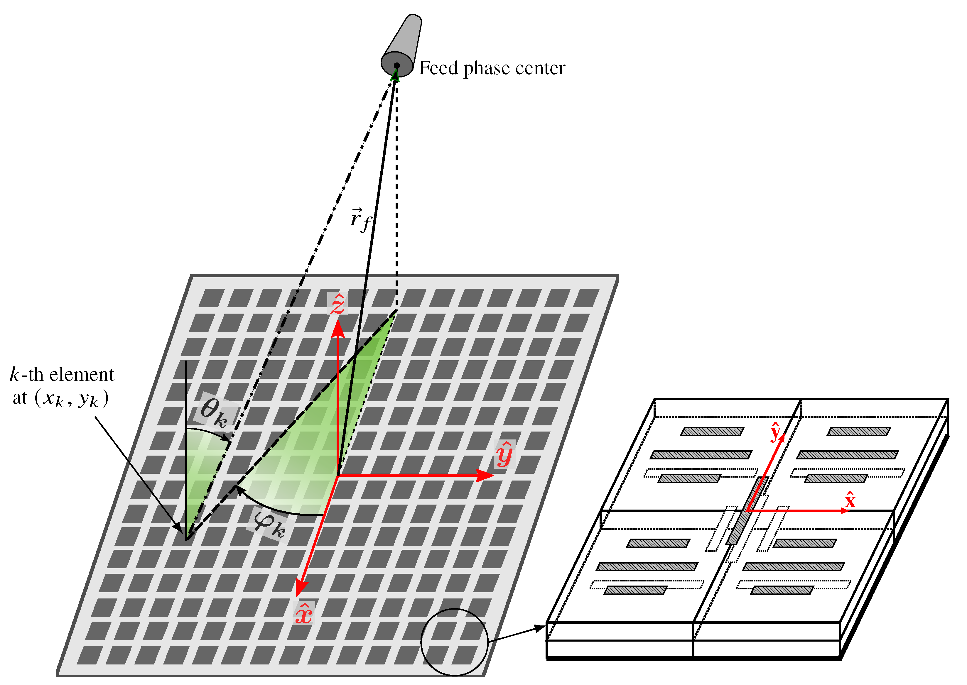
The main goal of employing a database for reflectarray analysis, layout design and direct layout optimization is to considerably accelerate those tasks with regard to the use of an FW-LP tool, while having a reasonable accuracy in the prediction of radiation patterns. Before detailing the particularities of the database, let us consider the reflectarray diagram shown in  Figure 1. The considered reflectarray is planar and composed of a number of elements or unit cells (depicted in  Figure 1 as patches, but other geometries are possible, such as dipoles, rings, etc.) and a feed of which the phase centre is placed at ${\overrightarrow{r}}_f$ with regard to the center of the reflectarray. With this antenna’s optics, the k-th element will experience an angle of incidence from the feed phase center $({\theta }_k,{\phi }_k)$, and it will be different for each reflectarray element.

The electromagnetic response of the k-th unit cell is given by the matrix of reflection coefficients, comprising four complex numbers:

$$R_k=\left(\begin{array}{cc}{\rho }_{xx,k}& {\rho }_{xy,k}\\ {\rho }_{yx,k}& {\rho }_{yy,k}\end{array}\right),$$

(1)

where ${\rho }_{xx}$ and ${\rho }_{yy}$ are known as the direct coefficients and ${\rho }_{xy}$ and ${\rho }_{yx}$ are known as the cross-coefficients. Their value depends on several parameters: frequency, periodicity of the unit cell, substrate characteristics, angle of incidence and the geometrical features of the unit cell (patch dimensions, dipole width and length, etc.). From the point of view of the antenna design, the frequency is fixed beforehand depending on the application, and it may be a certain bandwidth, in which case a small set of discrete frequencies are employed in the design. The substrate is also fixed and it is selected among a set of commercially available substrates. The periodicity may be chosen after a parametric study or to meet certain conditions, such as avoiding grating lobes [2]. The angles of incidence at each element are fixed once the antenna optics has been selected to meet certain requirements, such as gain and a lack of blockage by the feed (see  Figure 1). Finally, the geometrical features of the unit cell provide the degrees of freedom (DoF) for the reflectarray layout design and/or optimization.

Given the above-mentioned considerations, a database for the rapid calculation of the reflection coefficients in (1) should consider the frequencies of operation, the angle of incidence and the geometrical features of the unit cell. This means that the periodicity and substrate characteristics will be fixed before generating samples of R to populate the database. Thus, if either the periodicity or the substrate changes, the database needs to be generated again. However, once a database has been generated for a suitable unit cell, it can be reused in as many designs as necessary (the same would apply to MLT surrogate models).

After the database is generated and integrated into an analysis tool to obtain the reflection coefficients in (1), the radiation pattern can be computed by following the formulation detailed in [45].

3. Description of the Database

3.1. Structure of the Database

One important aspect to consider in relation to the database is how it is going to be stored and accessed in memory. Indeed, since the total number of entries in the database, $N_t$, may be very large, fast access to the sought database entries is relevant. In this regard, we generate the database for $N_f$ frequencies, $N_a$ angles of incidence $(\theta ,\phi )$ (as seen from the feed, see  Figure 1) and $N_g$ combinations of geometrical features (such as patch dimensions, dipole lengths, etc.). Thus, the total number of entries in the database would be:

$$N_t=N_f{N}_a{N}_g.$$

(2)

The database is stored in a rank-4 array, in which the first index refers to the reflection coefficient in (1), the second to the frequency, the third to the pair $(\theta ,\phi )$ and the fourth to the geometrical features of the unit cell. The frequencies are treated as discrete entities in the sense that no interpolation is performed to obtain reflection coefficients at frequencies that are not contained in the database. A similar approach is followed with the angles of incidence $(\theta ,\phi )$, which are discretized into a small set and then the real angle of incidence is approximated with one of the considered $(\theta ,\phi )$ pairs in the database. This approach was demonstrated in other works when working with SVR; see [41,44] for more details. Thus, the interpolation of the reflection coefficients is carried out only in regard to the geometrical features of the unit cell.

When using the database, the input variables are the working frequency, the real angle of incidence of the element (see  Figure 1) and the geometrical features of the unit cell. Since in general the input angle of incidence will not be stored in the database, a $(\theta ,\phi )$ pair will be chosen among the $N_a$ values stored in the database that is closest to the input angle of incidence. This is the same approach used in [44].

3.2. Fast Memory Access for the Reflection Coefficients

The determination of the index for the frequency and angle of incidence is not an issue since $N_f$ and $N_a$ are usually small numbers. In such a case, a linear search to choose them from a list of available frequencies and $(\theta ,\phi )$ pairs is sufficient. However, this is not the case with the geometrical features, since the number of total combinations $N_g$ grows exponentially with the number of degrees of freedom (DoFs) that the unit cell provides. Thus, a linear search over the $N_g$ entries to determine the reflection coefficients selected to carry out the interpolation would be too expensive, especially in the cases of layout design and crosspolar optimization where the database is used extensively (on the order of hundreds of thousands of times for large reflectarrays).

In order to find an efficient way to access the database, let us first establish some conditions on the entries of the database over the $N_g$ values. If the number of DoFs is D, since the interpolation is performed only over those D values, we will consider the dimensionality of the database to be D. For a given frequency and angle of incidence $(\theta ,\phi )$, we have a database generated in a regular grid with coordinates (or, equivalently, the physical dimensions of the geometrical features of the unit cell):

$$x_{i,k_i},i=1,2,\dots ,D;k_i=1,2,\dots ,N_{g_i},x_{i,k_i}\in {\mathbb{R}}^{+},$$

(3)

where index i refers to the dimension, $k_i$ is the index that runs over the $x_{i,k_i}$ values for a given dimension, and $N_{g_i}$ is the number of points in which the length of the i-th DoF is discretized. Note that $N_g={\prod }_{i=1}^D{N}_{g_i}$. In addition, the values $x_{i,k_i}$ have to comply with two conditions: they have to be monotonic, increasing for a given dimension i, and also regular in each dimension. These two conditions can be mathematically expressed as

$$\Delta x_{i,k_i}=x_{i,k_i+1}-x_{i,k_i}=c_i>0,\forall i=1,2,\dots ,D;\forall k_i=1,2,\dots ,N_{g_i}-1.$$

(4)

It is also important to point out that the $N_g$ entries of the database (for a given frequency and angle of incidence $(\theta ,\phi )$) are stored in such a way that $x_{i,k_i}$ varies faster in $k_i$ than $x_{i+1,k_i}$. For example, for the first $N_{g_1}$ values of the database, $x_{i,k_i}$ for $i\ge 2$ remain unchanged.

Given the above considerations, the fast memory access approach to find the reflection coefficients indices in the database is as follows:

• In the database initialization, we store D arrays with the values of the geometrical features of the unit cell (here called coordinates), where D is the number of DoFs. These values are denoted as $x_{i,k_i}$ [see (3)].
• The values $x_i^{*},i=1,2,\dots ,D$ correspond to the point at which we want to obtain the reflection coefficients. Note that the $x_i^{*}$ values are not generally stored in the database and thus an interpolation must be carried out.
• We employ a modified binary search (see Algorithm 1) in each dimension i to find an index $k_i$ such that:

  $$x_{i,k_i}\le x_i^{*}\le x_{i,k_i+1},i=1,2,\dots ,D.$$

  (5)
• Then, the general index of the reflection coefficient closest to the origin and which belongs to the hyper-rectangle bounding the point ${\overrightarrow{x}}^{*}=(x_1^{*},x_2^{*},\dots ,x_D^{*})$ is:

  $$k=1+\sum _{i=1}^D(k_i-1)\prod _{h=1}^{i-1}{N}_{g_h},$$

  (6)

  where the empty product (i.e., the product of zero numbers) is the multiplicative identity.

Notice that the indices $k_i$ may be employed not only to obtain index k to access the desired reflection coefficient, but also to obtain the coordinates $x_{i,k_i}$ and $x_{i,k_i+1}$, which are employed in the N-linear interpolation as described in the following subsection.

In point 3 above it is mentioned that a modified binary search is employed to find $k_i$. Indeed, the traditional binary search algorithm tries to find the exact value on a list [46]. However, in the present case we need to find an index $k_i$ such that the condition (5) holds. To that end, the binary search algorithm is modified as shown in Algorithm 1.

Algorithm 1. Modified binary search: given a sequence of ordered values $x_1<x_2<\cdots <x_N$ with regular spacing $\Delta x$ (i.e., fulfilling (4)) and a value $x^{*}\in \mathbb{R}$, the modified binary search finds the index $k\in \{1,2,\dots ,N\}$ such that $x_k\le x^{*}\le x_{k+1}$. If $x^{*}\notin [x_1,x_N]$, it returns $-1$, terminating unsuccessfully.

1: $l\leftarrow 1$                                         ▹ Initialization 2: $u\leftarrow N$ 3: while$l<u$do 4:     $k\leftarrow \lfloor (l+u)/2\rfloor$                                  ▹ Get the midpoint 5:     if $|x_k-x^{*}|>\Delta x$ then                                 ▹$x^{*}\notin [x_{k-1},x_{k+1}]$ 6:         if $x_k<x^{*}$ then 7:            $l\leftarrow k+1$ 8:         else 9:            $u\leftarrow k-1$ 10:         end if 11:     else                                        ▹$x^{*}\in [x_{k-1},x_{k+1}]$ 12:         if $x_k>x^{*}$ then 13:            return $k-1$                                   ▹$x^{*}\in [x_{k-1},x_k)$ 14:         else 15:            return k                                      ▹$x^{*}\in [x_k,x_{k+1}]$ 16:         end if 17:     end if 18: end while 19: return$-1$                            ▹$x^{*}\notin [x_1,x_N]$, terminates unsuccessfully

Finally, in order to accelerate the computation of the general index in (6), the product ${\prod }_{h=1}^{i-1}{N}_{g_h}$ may be precomputed in the database initialization, stored in an array of size D and accessed with index i to calculate (6). This precomputation is possible since the numbers $N_{g_i}$ are known beforehand.

3.3. N-Linear Interpolation

In general, the coordinates ${\overrightarrow{x}}^{*}$ of the interpolant are not stored in the database, and thus an interpolation needs to be performed. For this work, we have chosen a local N-linear interpolation since it is possibly the simplest and fastest way to interpolate data. Other works in the literature [30] have chosen local cubic interpolation on the basis that the scattering matrix has strong variation at resonance. The accuracy of the N-linear interpolation will be assessed in a subsequent section to elucidate if it is appropriate for reflectarray design and optimization. (Spoiler alert, it is suitable.)

Before introducing the mathematical formulation of the N-linear interpolation we need to briefly analyze some aspects of the grid in which the interpolation will be carried out. Furthermore, according to the notation employed in the previous subsection, $N=D$. Figure 2 gives three examples of grids for $D=1,2,3$ that comply with (4), including a point ${\overrightarrow{x}}^{*}$ where the interpolant is to be calculated. As can be seen, when we want to use the database to retrieve the reflection coefficients with coordinates ${\overrightarrow{x}}^{*}$, the database needs to identify $2^D$ entries, corresponding to each of the vertices of the hyper-rectangle (or, more formally, D-orthotope) surrounding ${\overrightarrow{x}}^{*}$. However, given the condition in (4), we only need to identify the vertex that is closest to the origin, or more specifically, its index for each dimension, $k_i$. The rest of the vertices of the hyper-rectangle can be obtained from the indices of the vertex closest to the origin by adding one to the relevant $k_i$.

The general equation for the interpolation is [47]:

$$f\left({\overrightarrow{x}}^{*}\right)=\sum _{u=0}^{2^D-1}{\rho }_{(k_1+b_1\left(u\right),\dots ,k_D+b_D\left(u\right))}\prod _{i=1}^D{W}_i^{b_i\left(u\right)},$$

(7)

where ${\overrightarrow{x}}^{*}=(x_1^{*},x_2^{*},\dots ,x_D^{*})$ are the coordinates of the desired interpolated reflection coefficient and they correspond to the physical lengths of the geometrical features of the unit cell; $b_i\left(u\right)$ is a function that gives the i-th bit of the integer number u; $\rho$ is the selected reflection coefficient for a given u and indices $k_i$ (or more specifically, its real or imaginary part); and $W_i$ is the weighting vector

$$W_i=\left(1-w_i\left(x_i^{*}\right),w_i\left(x_i^{*}\right)\right),$$

(8)

where

$$w_i\left(x_i^{*}\right)=\frac{x_i^{*}-x_{i,k_i}}{x_{i,k_i+1}-x_{i,k_i}}.$$

(9)

A clarification about the notation of $\rho$ and $W_i$ in (7) regarding the sub- and super-scripts is in order. First, in the case of $W_i^{b_i\left(u\right)}$, the sub-script indicates the current dimension, while the super-script refers to the indization of the array in (8), which has been indexed such as the first component has index zero. Since the function $b_i\left(u\right)$ returns a bit, which can only be 0 or 1, either $W_i^0=1-w_i\left(x_i^{*}\right)$ or $W_i^1=w_i\left(x_i^{*}\right)$ are selected depending on the value of the indices i and u to find the product ${\prod }_{i=1}^D{W}_i^{b_i\left(u\right)}$.

The reflection coefficient $\rho$ in (7) is indexed with the following notation:

$$(k_1+b_1\left(u\right),k_2+b_2\left(u\right),\dots ,k_D+b_D\left(u\right)).$$

(10)

as we recall from the previous subsection, $k_i$ are the indices, found using Algorithm 1 for each dimension i, that correspond to the coordinates that bound (i.e., directly above and below, see (5)) the desired coordinate $x_i^{*}$ where we want to interpolate the reflection coefficient. In a space of D dimensions, we consider a hyper-rectangle of $2^D$ vertices, which is employed to carry out the interpolation with (7). The indices of the vertex closest to the origin would be $(k_1,k_2,\dots ,k_D)$, and it corresponds to $u=0$, since its binary representation is all zeros. Then, we follow the rest of the vertices in lexicographical order by considering the binary pattern of a number $u=0,1,\dots ,2^D-1$ comprised of D bits. With this idea and using (10) to index the reflection coefficients, we define a new index,

$${\tilde{k}}_i\left(u\right)=k_i+b_i\left(u\right),$$

(11)

which in combination with (6) can be used to find the general index of the $2^D$ vertices as

$$k\left(u\right)=1+\sum _{i=1}^D[{\tilde{k}}_i\left(u\right)-1]\prod _{h=1}^{i-1}{N}_{g_h}.$$

(12)

in this way, using (12) we find the reflection coefficient $\rho$ to perform the interpolation with (7). Notice that the binary search only needs to be performed once per dimension (and not $2^D$ times per dimension) to find $k_i$ for the vertex closest to the origin. The rest of the vertices are calculated with (12) once $k_i$ are known.

Finally, it is worth mentioning that since the four reflection coefficients are complex numbers, the multidimensional linear interpolation is applied to their real and imaginary parts, in such a way that (7) is applied eight times every time the database is invoked. Furthermore, more accuracy may be achieved by directly interpolating the magnitude of the direct coefficients instead of obtaining it from the interpolated real and imaginary part. In such case, the interpolation would be applied ten times every time the database is used. This is the approach followed in this work, and it was also followed to obtain the surrogate models using SVR [40].

3.4. Visual Representation of Multilinear Interpolation for Low Dimensions

Figure 3 shows three examples of the multi-linear interpolation in one, two and three dimensions. These are also known as linear, bilinear and trilinear interpolations. In the case of the linear interpolation (Figure 3a), the original data are represented by the blue points, and the interpolation generates the straight lines that join the dots. Indeed, if (7) is employed for $D=1$ we get:

$$f\left(x\right)={\rho }_k[1-w\left(x\right)]+{\rho }_{k+1}w\left(x\right),$$

(13)

where $w\left(x\right)$ is defined in (9). This equation corresponds to a straight line that joins the points $(x_k,{\rho }_k)$ and $(x_{k+1},{\rho }_{k+1})$, and then the data are averaged with functions $[1-w(x\left)\right]$ and $w\left(x\right)$, which depend on how far or close coordinate x is from $x_k$ and $x_{k+1}$.

Figure 3b plots an example of bilinear interpolation that is carried out in a unit square with the original data lying in the vertices of the square with values 0, 0.8, 0.5 and 0.8 in clockwise order. The inset shows a top view of the unit square. Particularizing (7) for two dimensions we get:

$$\begin{array}{cc}\hfill f(x_1,x_2)& ={\rho }_{(k_1,k_2)}[1-w_1\left(x_1\right)][1-w_2\left(x_2\right)]+{\rho }_{(k_1+1,k_2)}{w}_1\left(x_1\right)[1-w_2\left(x_2\right)]\hfill \\ \hfill & \phantom{=}+{\rho }_{(k_1,k_2+1)}[1-w_1\left(x_1\right)]w_2\left(x_2\right)+{\rho }_{(k_1+1,k_2+1)}{w}_1\left(x_1\right)w_2\left(x_2\right),\hfill \end{array}$$

(14)

which defines the surface shown in Figure 3b. Note that, in this case, the interpolated value is given by both the z-axis and the color gradient.

A trilinear interpolation is shown in Figure 3c. This time, it is carried out in a unit cube. The original data values for the bottom vertices are the same as for the upper vertices, 0, 0.8, 0.5 and 0.8 in clockwise order (the same as the bilinear interpolation). Since the interpolation is also performed inside the cube, Figure 3c also shows the three middle inner slices. In this case, the interpolated values can only be shown with the color gradient, since the three orthogonal axes are employed for the coordinates.

4. Results

4.1. Testing Conditions

To test the proposed database, the same large rectangular reflectarray as that analyzed in [41] is employed for a fair comparison with other techniques. It is composed of 7052 elements, and a contoured beam pattern in dual-linear polarization was selected to assess the accuracy at the radiation pattern level. In addition, the same unit cell is employed, which consists in eight coplanar and parallel dipoles, four for each polarization. This unit cell is shown in Figure 1. For the sake of comparison with other works, we reduce the number of DoFs to two by imposing a scaling between parallel dipoles as in [41], thus having $N=D=2$. These DoFs are denoted as $T_x$ and $T_y$, controlling linear polarizations X and Y, respectively.

In order to compare the accuracy and computing performance of the database, the SVR-based analysis technique described in [40] is employed, with the same 2D SVR used in [41]. The MoM-LP employed as baseline and used to populate the database and generate the training samples of the SVR is fully described in [21]. The total numbers of samples for the database and the SVR are the same, at 380,000 ($N_f=1$, $N_a=152$, $N_{g_1}=N_{g_2}=50$, $N_g=N_{g_1}{N}_{g_2}$).

The three tools (database, SVR and MoM-LP) will be compared for three different tasks: obtaining a reflectarray layout such that it generates the desired phase-shift distribution, performing a single analysis of a reflectarray layout and carrying out a direct layout optimization for crosspolar optimization.

To assess the computing efficiency, an Intel i9-9900 CPU working at 3.1 GHz and with 32 GB of memory was employed. All computations were parallelized, employing the maximum number of threads allowed by this CPU using hyper-threading.

4.2. Reflection Coefficients

The final goal of the comparison between the different analysis tools is the simulated radiation pattern, since the performance of the antenna is based on parameters in the far field. However, the most immediate result of the database and the surrogate model based on SVR is the reflection coefficients in (1). Figure 4 shows a visual comparison of two reflection coefficients, ${\rho }_{xx}$ and ${\rho }_{xy}$, in magnitude and phase at oblique incidence $(\theta ,\phi )=$ (29°, 35°). As can be seen, the phase curve of the direct coefficient ${\rho }_{xx}$ is predicted with a high degree of accuracy by the database. Since the phase of the direct coefficients is the only parameter employed in the layout design of reflectarray antennas [2,26], this means that the database presents a low degree of error when performing a layout design. The magnitude of ${\rho }_{xx}$, as well as the cross-coefficient, are also predicted with a high degree of accuracy.

4.3. Layout Design

For the layout design we considered the phase distribution shown in Figure 5. It was obtained using a phase-only synthesis algorithm, namely, the generalized intersection approach [26] to provide a European coverage from a geostationary satellite [41]. From this phase distribution, the layout was obtained by following the procedure detailed in [37], which can be summarized in the following three steps: (1) generating a phase-shift table for each linear polarization; (2) using a linear equation approximation to find the desired geometrical unit cell length for each polarization independently; (3) fine-tuning the geometrical length of both polarizations at the same time by employing the Newton–Raphson gradient method. This methodology was applied with the three tools and the computing performance can be seen in

Table 1. Performance of the proposed database with regard to SVR and MoM-LP tools for layout design.

Tool	Time (s)	Speed-Up
MoM-LP	1572.55	1
SVR	1.11	1417
Database	0.04	39,314

. As can be seen, both the database and the SVR tool are substantially faster than the MoM-LP, but the database is an order of magnitude faster than the SVR for this task.

For the layout design, the accuracy was analyzed from two different perspectives. First, Figure 6 shows the relative error in the obtained design when using the database and the SVR tool compared to the design obtained with MoM-LP. As can be seen, the relative error for both tools was very low and of the same order, confirming the accuracy of the proposed database. Figure 7 shows the real layout obtained with the database using the unit cell of Figure 1. Since this unit cell has the dipoles in two layers of metallizations, Figure 7 shows both layers.

Second, we need to assess if those differences in the designed layout have any repercussions on the radiation pattern. To that end, each layout was simulated with the MoM-LP tool and the main figures of merit were compared for both linear polarizations. These are, for the coverage zone: minimum copolar gain (CP_min), minimum crosspolar discrimination (XPD_min) and crosspolar isolation (XPI). The definitions of XPD_min and XPI can be found elsewhere [48]. The results are provided in

Table 2. Figures of merit of a European coverage pattern when the design is carried out using different tools and simulated with MoM-LP. CP_min is in dBi and XPD_min and XPI are in dB.

	Polarization X			Polarization Y
Design Tool	CPmin	XPDmin	XPI	CPmin	XPDmin	XPI
MoM-LP	30.03	32.95	32.91	30.02	32.94	32.90
Database	30.03	32.97	32.92	30.01	32.95	32.90
SVR	30.03	32.95	32.90	30.00	32.94	32.88

. As can be seen, the differences in the figures of merit are negligible, proving that the small differences in the layout design shown in Figure 6 barely affect the radiation pattern in the coverage zone. Indeed, the relative error of the radiation pattern obtained with the design carried out with the database compared with that of the design obtained with MoM-LP is smaller than 0.2% for the copolar pattern and smaller than 0.7% for the crosspolar pattern.

4.4. Reflectarray Analysis

The previous assessment compared the radiation patterns when three different layouts obtained with MoM-LP, SVR and the database were simulated with the same tool, namely MoM-LP. In this way, we could determine the accuracy of the database to perform a layout design. Next, we assessed the accuracy in the analysis of a given layout. To that end, the layout obtained with the database in the previous subsection was selected and simulated with the three tools to compare again the three figures of merit. These results are gathered in

Table 3. Figures of merit of a European coverage pattern when the design is carried out using the database and simulated with different tools. CP_min is in dBi and XPD_min and XPI are in dB.

	Pol. X			Pol. Y
Analysis Tool	CPmin	XPDmin	XPI	CPmin	XPDmin	XPI
MoM-LP	30.03	32.97	32.92	30.01	32.95	32.90
Database	30.03	32.88	32.65	30.02	32.67	32.63
SVR	30.03	32.80	32.58	30.02	32.79	32.76

. In this case, there are more differences in the values of the figures of merit, especially for the crosspolar discrimination and isolation, although they are still very small. The largest difference is for XPI with a difference of 0.27 dB between the simulations using the database and MoM-LP. However, comparing the database and the SVR simulations, the figures of merit are very similar. This is due to the error in the radiation pattern produced by the discretization of the angles of incidence, which has been thoroughly studied in [44].

Figure 8 shows a visual comparison of the radiation pattern obtained in the analyses carried out with MoM-LP, the database and SVR. This radiation pattern is the same pattern used to collect the data in Table 3. As can be seen, the simulations with the database and SVR offer virtually the same results, and both simulations fit with a high degree of accuracy that of the MoM-LP for the copolar pattern. In the case of the crosspolar pattern there are some important discrepancies for levels around −20 dBi, but these levels are 50 dB below the peak gain. More importantly, for higher crosspolar values around and within the coverage area, the database offers good accuracy when compared with the MoM-LP simulation.

4.5. Direct Layout Optimization for Cross-Polarization Improvement

Once we established the accuracy of the database for the analysis and layout design of reflectarray antennas, we tested its suitability for a direct layout optimization process, employing the algorithm described in [49] and particularized for reflectarray antennas in [26]. As a starting point for the optimization, the layout designed using the database was used. Thus, the starting values for CP_min, XPD_min and XPI are the ones shown in the first row of Table 3. In addition, for the sake of comparison, three optimizations were performed, one with each tool. The goal of the optimization was to improve the cross-polarization performance of the antenna, XPD_min and XPI, while preserving the copolar pattern. To that end, the XPD_min and XPI parameters were set to 40 dB in the optimization algorithm. Moreover, the three optimizations were stopped after 16 iterations of the generalized Intersection approach and the resulting layout was simulated, in all cases, with the MoM-LP tool to assess the difference in performing the optimization with each tool, removing the differences in the final analysis, which was already assessed in the previous subsection.

From a computing time perspective, the use of the database showed a similar performance to that given by the SVR, as shown in

Table 4. Computing time performance of the direct layout optimization considering three different tools for the analysis of the reflectarray unit cell. Time is in seconds.

Tool	Time Per Iteration	Jacobian Time
MoM-LP	69.39	34.06
SVR	5.00	2.31
Database	4.86	2.20

. The mean time per iteration and the time to compute the Jacobian matrix were very similar using both tools. The explanation for this phenomenon, given that the database is significantly faster than the SVR for analysis and layout design, comes from the fact that both tools are so fast that the dominant time to perform the computation of the Jacobian matrix comes from the rest of the operations, which also involve the computation of the radiation pattern and the figures of merit for both linear polarizations.

Table 5. Comparison of the figures of merit of a European-coverage pattern after direct layout optimization to improve cross-polarization performance. Three optimizations were carried out with different tools, setting the the goal for XPD_min and XPI to 40 dB. In all cases, the layout after 16 iterations of the optimization algorithm was simulated with MoM-LP. For optimization with the database, results are also shown when the result was simulated with the database. CP_min is in dBi and XPD_min and XPI are in dB.

		Pol. X			Pol. Y
Opt. Tool	Sim. Tool	CPmin	XPDmin	XPI	CPmin	XPDmin	XPI
MoM-LP	MoM-LP	29.90	39.80	39.62	30.01	40.07	39.93
Database	MoM-LP	29.93	38.69	38.63	30.01	39.38	39.08
Database	Database	29.94	39.72	39.60	30.01	40.19	39.88
SVR	MoM-LP	29.94	38.74	38.65	30.01	39.14	38.87

shows the results of the three optimized layouts simulated with MoM-LP. As can be seen, in all cases the cross-polarization performance of the reflectarray was considerably improved, while preserving the copolar pattern. The cross-polarization figures of merit after the optimization with the database and the SVR are similar, and in both cases lower than those obtained with MoM-LP. The table also includes the results when the layout optimized with the database is also simulated with the database (row three). Comparing rows two and three of Table 5 it can be seen that the values for the cross-polarization figures of merit are not as good. In fact, since this is a comparison between MoM-LP and the database, one would expect differences such as the ones shown in Table 3, where the differences where smaller than 0.3 dB, whereas in Table 5 they are around 1 dB. The reason for this discrepancy is the higher sensitivity of the crosspolar pattern when the values are very low to the discretization of the angles of incidence [44]. Indeed, a similar phenomenon was detected in [37] when using SVR in the optimization. In any case, when considering the simulation with MoM-LP and the real angles of incidence, the improvement in cross-polarization is patent, regardless of the tool used.

Despite the small differences, the use of the database for analysis, layout design and crosspolar optimization remained highly accurate, while considerably reducing computing times with regard to the use of the MoM-LP tool, and did not require the training process that any machine learning technique must go through. The studies carried out in this work were performed for databases and SVR considering two DoFs ($D=2$), one per polarization. It is possible that higher-dimensionality machine learning techniques may require far fewer training samples than a database to maintain the desired accuracy [41]. However, this would require tackling the problem of the resonances that may appear in the reflection coefficients for successful training, which is averted in the database at the potential expense of an exponential increase in the number of samples (i.e., database entries).

5. Reducing the Number of Samples in the Database

The results shown in the previous section demonstrate the discrepancies in the radiation patterns for different tasks: layout design, antenna analysis and direct layout optimization. As long as the analysis is accurate enough, the layout design and optimization will provide accurate results as well. However, the accuracy of the database not only depends on the interpolation approach used (N-linear in the present work), but also on the number of samples employed to populate the database. For instance, here $N_{g_1}=N_{g_2}=50$ yielded very accurate results. Other works employ more samples in each dimension, such as $N_{g_i}=60$ in [30]. In the case of surrogate models based on SVR, one can considerably reduce the number of training samples without affecting the accuracy of the radiation pattern [41]. This also implies the opposite: there is a point from which it does not matter how many more training samples are employed; the accuracy will not improve. Thus, it is also interesting to analyze how modifying the sample density in the database impacts the accuracy at the radiation pattern level.

For a fair comparison with the surrogate models, we employed the same number of samples in our database as that used by the SVR in the training process. That means that the samples used in the test phase of the cross-validation procedure were not counted towards the total number of samples used to populate the database. It is worth noting that only the number of samples in the database and the SVR training process was the same—not the samples themselves, since the database requires a regular grid, whereas the SVR employs randomly generated samples [40].

For this comparison, the following relative error in the radiation pattern was used:

$${\mathrm{RE}}_{\mathrm{FF}}=100·{\displaystyle \frac{\parallel G_{\mathrm{MoM}-\mathrm{LP}}-G_{\mathrm{SVR}\mathrm{or}\mathrm{Database}}\parallel }{\parallel G_{\mathrm{MoM}-\mathrm{LP}}\parallel }}(\%),$$

(15)

where G is either the copolar or the crosspolar gain pattern. Note that, using the ${\ell }^2$-norm in (15), all the points at which the far field is computed are taken into account for the calculation of the relative error. This means that the side-lobe area will contribute to the error as much as points in the coverage zone where the figures of merit are computed (i.e., CP_min, XPD_min and XPI).

Figure 9 shows the evolution of the relative error of the radiation pattern when the number of samples varies. For the database it includes two lines. The solid line represents the evolution of the relative error when the magnitude of the direct coefficients ${\rho }_{xx}$ and ${\rho }_{yy}$ is directly interpolated, whereas the dashed line represents the relative error when the magnitudes of ${\rho }_{xx}$ and ${\rho }_{yy}$ are obtained from the interpolated real and imaginary parts. As can be seen, directly interpolating the magnitude of the direct coefficients significantly increases the overall accuracy of the database, making it more robust and accurate when the number of samples per $(\theta ,\phi )$ pair decreases. Indeed, in that case, the relative error of the database and the surrogate models based on SVR is very similar for both the copolar and crosspolar components of the radiation pattern.

In addition, the relevant figures of merit did not change very significantly.

Table 6. Comparison of the figures of merit of a European-coverage pattern for different values in the total number of database entries $N_g=N_{g_1}{N}_{g_2}$. CP_min is in dBi and XPD_min and XPI are in dB.

		Polarization X			Polarization Y
Tool	${\mathit{N}}_{{\mathit{g}}_1}\times {\mathit{N}}_{{\mathit{g}}_2}$	CPmin	XPDmin	XPI	CPmin	XPDmin	XPI
MoM-LP	—	30.03	32.97	32.92	30.01	32.95	32.90
Database	$46\times 46$	30.03	32.90	32.67	30.02	32.64	32.60
Database	$30\times 30$	30.03	33.04	32.81	30.02	32.35	32.31

shows the values of the figures of merit for two different databases employed to generate Figure 9, specifically, the rightmost point ($46\times 46$) and the third point from the left ($30\times 30$). As reference, the figures of merit obtained in a simulation with MoM-LP are also provided. As can be seen, even when significantly reducing the number of samples in the database, from a grid of $46\times 46$ points to $30\times 30$, the value of the figures of merit barely change. This result is in agreement with that shown in Figure 9, and it can be exploited for high-dimensional databases to greatly reduce the total number of samples by reducing the size of the grid, while still obtaining acceptable accuracy in the radiation pattern.

6. Conclusions

In this work, we have presented a simple and efficient database for reflectarray analysis, layout design and direct layout optimization for cross-polarization improvement. The database employs multidimensional N-linear interpolation and efficient access to the reflection coefficients stored in the memory for a very fast analysis of the unit cell.

In order to assess the performance of this database both in terms of computational efficiency and accuracy at the radiation pattern level, it was compared with the MoM-LP tool employed to populate the database and with a machine learning technique based on SVR. In all cases shown in this work, the database presents a high degree of accuracy compared with the simulations carried out with MoM-LP, while significantly decreasing computing times. In particular, the database is four orders of magnitude faster than MoM-LP in carrying out analysis and layout design, whereas it is an order of magnitude faster than the SVR for the same tasks. In addition to this improved computational performance in reflectarray analysis and design, the accuracy remains high, with a relative difference in the obtained layout of less than 1.1%, which translates to relative errors in the radiation pattern of less 0.2% in the copolar pattern and less than 0.7% in the radiation pattern. Regarding the accuracy in the figures of merit, differences in minimum copolar gain in the area of interest are negligible, whereas in the cross-polarization performance the maximum difference was less than 0.3 dB in the XPI parameter. For direct layout optimization, both the database and the SVR offered similar computing times with similar accuracy, both being one order of magnitude faster than the MoM-LP approach.

In addition, the database accuracy as a function of the number of samples per pair of angles of incidence was tested. As is the case with SVR models, the number of samples can be reliably reduced while maintaining a high degree of accuracy in the radiation pattern. This behavior is very interesting for high-dimensional databases, since the number of samples quickly increases with the dimensionality. Thus, by maintaining a low sample density in each dimension, the total number of samples can be kept to a moderate number without excessively penalizing the accuracy in the prediction of the radiation patterns.

The use of the database, despite using a simple N-linear interpolation, offers good accuracy and fast computing times compared to the use of MoM-LP. Compared to machine learning techniques such as SVR, it avoids the training phase, which can be time consuming. Thus, a database based on N-linear interpolation is a suitable tool for reflectarray design and direct layout optimization for any application that requires the use of this kind of antenna.

References

1. Berry, D.G.; Malech, R.G.; Kennedy, W.A. The reflectarray antenna. IEEE Trans. Antennas Propag. 1963, 11, 645–651. [Google Scholar] [CrossRef]
2. Huang, J.; Encinar, J.A. Reflectarray Antennas; John Wiley & Sons: Hoboken, NJ, USA, 2008. [Google Scholar]
3. Nayeri, P.; Yang, F.; Elsherbeni, A.Z. Reflectarray Antennas: Theory, Designs, and Applications; John Wiley & Sons: Hoboken, NJ, USA, 2018. [Google Scholar]
4. Imbriale, W.A.; Gao, S.; Boccia, L. (Eds.) Space Antenna Handbook; John Wiley & Sons: Hoboken, NJ, USA, 2012. [Google Scholar] [CrossRef]
5. Encinar, J.A.; Datashvili, L.S.; Zornoza, J.A.; Arrebola, M.; Sierra-Castaner, M.; Besada-Sanmartin, J.L.; Baier, H.; Legay, H. Dual-Polarization Dual-Coverage Reflectarray for Space Applications. IEEE Trans. Antennas Propag. 2006, 54, 2827–2837. [Google Scholar] [CrossRef]
6. Hodges, R.E.; Chahat, N.; Hoppe, D.J.; Vacchione, J.D. A Deployable High-Gain Antenna Bound for Mars: Developing a new folded-panel reflectarray for the first CubeSat mission to Mars. IEEE Antennas Propag. Mag. 2017, 59, 39–49. [Google Scholar] [CrossRef]
7. De Rioja, E.M.; de Rioja, D.M.; López-Sáez, R.; Linares, I.; Encinar, J.A. High-Efficiency Polarizer Reflectarray Antennas for Data Transmission Links from a CubeSat. Electronics 2021, 10, 1802. [Google Scholar] [CrossRef]
8. Rengarajan, S.R. Reflectarrays of rectangular microstrip patches for dual-polarization dual-beam radar interferometers. Prog. Electromagn. Res. 2013, 133, 1–15. [Google Scholar] [CrossRef] [Green Version]
9. Prado, D.R.; Campa, A.; Arrebola, M.; Pino, M.R.; Encinar, J.A.; Las-Heras, F. Design, manufacture and measurement of a low-cost reflectarray for global Earth coverage. IEEE Antennas Wirel. Propag. Lett. 2016, 15, 1418–1421. [Google Scholar] [CrossRef] [Green Version]
10. Zhou, M.; Sørensen, S.B.; Brand, Y.; Toso, G. Doubly Curved Reflectarray for Dual-Band Multiple Spot Beam Communication Satellites. IEEE Trans. Antennas Propag. 2020, 68, 2087–2096. [Google Scholar] [CrossRef]
11. De Rioja, D.M.; de Rioja, E.M.; Rodriguez-Vaqueiro, Y.; Encinar, J.A.; Pino, A.; Arias, M.; Toso, G. Transmit–Receive Parabolic Reflectarray to Generate Two Beams per Feed for Multispot Satellite Antennas in Ka-Band. IEEE Trans. Antennas Propag. 2021, 69, 2673–2685. [Google Scholar] [CrossRef]
12. Arrebola, M.; Encinar, J.A.; Barba, M. Multifed Printed Reflectarray With Three Simultaneous Shaped Beams for LMDS Central Station Antenna. IEEE Trans. Antennas Propag. 2008, 56, 1518–1527. [Google Scholar] [CrossRef]
13. Shen, Y.; Hu, S.; Dou, W. 38 GHz folded reflectarray antenna for point-to-point 5G communications. In Proceedings of the IEEE 5th Asia-Pacific Conference on Antennas and Propagation (APCAP), Kaohsiung, Taiwan, 26–29 July 2016; pp. 369–370. [Google Scholar] [CrossRef]
14. Yu, Z.Y.; Zhang, Y.H.; He, S.Y.; Gao, H.T.; Chen, H.T.; Zhu, G.Q. A Wide-Angle Coverage and Low Scan Loss Beam Steering Circularly Polarized Folded Reflectarray Antenna for Millimeter-Wave Applications. IEEE Trans. Antennas Propag. 2021. early access. [Google Scholar] [CrossRef]
15. Pérez-Adán, D.; Fresnedo, O.; González-Coma, J.P.; Castedo, L. Intelligent Reflective Surfaces for Wireless Networks: An Overview of Applications, Approached Issues, and Open Problems. Electronics 2021, 10, 2345. [Google Scholar] [CrossRef]
16. Maruyama, T.; Chen, Q.; Suematsu, N. Applied Reflectarray based on Metasurface for Wireless Power Transmission Efficiencys. In Proceedings of the 23rd International Conference on Applied Electromagnetics and Communications (ICECOM), Dubrovnik, Croatia, 30 September–2 October 2019; pp. 1–2. [Google Scholar] [CrossRef]
17. Maruyama, T.; Nakatsugawa, M.; Suematsu, N.; Motoyoshi, M.; Chen, Q.; Sato, H.; Omiya, M. Novel Design of Rectenna Array Using Metasurface for IoT. In Proceedings of the IEEE-APS Topical Conference on Antennas and Propagation in Wireless Communications (APWC), Honolulu, HI, USA, 9–13 August 2021; pp. 165–167. [Google Scholar] [CrossRef]
18. Vaquero, A.F.; Arrebola, M.; Pino, M.R.; Florencio, R.; Encinar, J.A. Demonstration of a Reflectarray with Near-field Amplitude and Phase Constraints as Compact Antenna Test Range Probe for 5G New Radio Devices. IEEE Trans. Antennas Propag. 2021, 69, 2715–2726. [Google Scholar] [CrossRef]
19. Pozar, D.M.; Targonski, S.D.; Syrigos, H.D. Design of millimeter wave microstrip reflectarrays. IEEE Trans. Antennas Propag. 1997, 45, 287–296. [Google Scholar] [CrossRef]
20. Encinar, J.A. Design of two-layer printed reflectarrays using patches of variable size. IEEE Trans. Antennas Propag. 2001, 49, 1403–1410. [Google Scholar] [CrossRef]
21. Florencio, R.; Boix, R.R.; Encinar, J.A. Enhanced MoM Analysis of the Scattering by Periodic Strip Gratings in Multilayered Substrates. IEEE Trans. Antennas Propag. 2013, 61, 5088–5099. [Google Scholar] [CrossRef]
22. Camacho, M.; Boix, R.R.; Medina, F. NUFFT for the Efficient Spectral Domain MoM Analysis of a Wide Variety of Multilayered Periodic Structures. IEEE Trans. Antennas Propag. 2019, 67, 6551–6563. [Google Scholar] [CrossRef]
23. De Vita, P.; Freni, A.; Vipiana, F.; Pirinoli, P.; Vecchi, G. Fast Analysis of Large Finite Arrays With a Combined Multiresolution–SM/AIM Approach. IEEE Trans. Antennas Propag. 2006, 54, 3827–3832. [Google Scholar] [CrossRef]
24. González, I.; Tayebi, A.; Gomez, J.; Delgado, C.; Cátedra, F. Fast Analysis of a Dual-Band Reflectarray Using Two Different Numerical Approaches Based on the Moment Method. IEEE Trans. Antennas Propag. 2013, 61, 2333–2336. [Google Scholar] [CrossRef]
25. Prado, D.R.; Arrebola, M.; Pino, M.R.; Goussetis, G. Contoured-Beam Dual-Band Dual-Linear Polarized Reflectarray Design Using a Multi-Objective Multi-Stage Optimization. IEEE Trans. Antennas Propag. 2020, 68, 7682–7687. [Google Scholar] [CrossRef]
26. Prado, D.R.; López-Fernández, J.A.; Arrebola, M.; Pino, M.R.; Goussetis, G. General Framework for the Efficient Optimization of Reflectarray Antennas for Contoured Beam Space Applications. IEEE Access 2018, 6, 72295–72310. [Google Scholar] [CrossRef]
27. Zhou, M.; Sørensen, S.B.; Kim, O.S.; Jørgensen, E.; Meincke, P.; Breinbjerg, O. Direct Optimization of Printed Reflectarrays for Contoured Beam Satellite Antenna Applications. IEEE Trans. Antennas Propag. 2013, 61, 1995–2004. [Google Scholar] [CrossRef] [Green Version]
28. Niccolai, A.; Beccaria, M.; Zich, R.E.; Massaccesi, A.; Pirinoli, P. Social Network Optimization Based Procedure for Beam-Scanning Reflectarray Antenna Design. IEEE Open J. Antennas Propag. 2020, 1, 500–512. [Google Scholar] [CrossRef]
29. Beccaria, M.; Niccolai, A.; Zich, R.E.; Pirinoli, P. Shaped-Beam Reflectarray Design by Means of Social Network Optimization (SNO). Electronics 2021, 10, 744. [Google Scholar] [CrossRef]
30. Zhou, M.; Sørensen, S.B.; Kim, O.S.; Jørgensen, E.; Meincke, P.; Breinbjerg, O.; Toso, G. The Generalized Direct Optimization Technique for Printed Reflectarrays. IEEE Trans. Antennas Propag. 2014, 62, 1690–1700. [Google Scholar] [CrossRef] [Green Version]
31. Abdallah, Y.; Menudier, C.; Thevenot, M.; Monediere, T. Synthesis of reflectarrays with mutual couplings. In Proceedings of the 7th European Conference on Antennas and Propagation (EuCAP), Gothenburg, Sweden, 8–12 April 2013; pp. 3446–3450. [Google Scholar]
32. Capozzoli, A.; Curcio, C.; Liseno, A.; Migliorelli, M.; Toso, G. Fast analysis and database generation in aperiodic reflectarrays. In Proceedings of the 7th European Conference on Antennas and Propagation (EuCAP), Gothenburg, Sweden, 8–12 April 2013; pp. 3913–3916. [Google Scholar]
33. Robustillo, P.; Zapata, J.; Encinar, J.A.; Rubio, J. ANN Characterization of Multi-Layer Reflectarray Elements for Contoured-Beam Space Antennas in the Ku-Band. IEEE Trans. Antennas Propag. 2012, 60, 3205–3214. [Google Scholar] [CrossRef]
34. Freni, A.; Mussetta, M.; Pirinoli, P. Neural network characterization of reflectarray antennas. Int. J. Antennas Propag. 2012, 2012, 541354. [Google Scholar] [CrossRef]
35. Richard, V.; Loison, R.; Gillard, R.; Legay, H.; Romier, M.; Martinaud, J.P.; Bresciani, D.; Delepaux, F. Spherical Mapping of the Second-Order Phoenix Cell for Unbounded Direct Reflectarray Copolar Optimization. Prog. Electromagn. Res. C 2019, 90, 109–124. [Google Scholar] [CrossRef] [Green Version]
36. Oliveri, G.; Gelmini, A.; Polo, A.; Anselmi, N.; Massa, A. System-by-Design Multiscale Synthesis of Task-Oriented Reflectarrays. IEEE Trans. Antennas Propag. 2020, 68, 2867–2882. [Google Scholar] [CrossRef]
37. Prado, D.R.; López-Fernández, J.A.; Arrebola, M.; Goussetis, G. Support Vector Regression to Accelerate Design and Crosspolar Optimization of Shaped-Beam Reflectarray Antennas for Space Applications. IEEE Trans. Antennas Propag. 2019, 67, 1659–1668. [Google Scholar] [CrossRef] [Green Version]
38. Shi, L.; Zhang, Q.; Zhang, S.; Yi, C.; Liu, G. Electromagnetic Response Prediction of Reflectarray Antenna Elements Based on Support Vector Regression. Appl. Comput. Electromagn. Soc. J. 2020, 35, 1519–1524. [Google Scholar] [CrossRef]
39. Schölkopf, B.; Smola, A.J. Learning with Kernels, 1st ed.; The MIT Press: Cambridge, MA, USA, 2001. [Google Scholar]
40. Prado, D.R.; López-Fernández, J.A.; Barquero, G.; Arrebola, M.; Las-Heras, F. Fast and Accurate Modeling of Dual-Polarized Reflectarray Unit Cells Using Support Vector Machines. IEEE Trans. Antennas Propag. 2018, 66, 1258–1270. [Google Scholar] [CrossRef]
41. Prado, D.R.; López-Fernández, J.A.; Arrebola, M.; Goussetis, G. On the Use of the Angle of Incidence in Support Vector Regression Surrogate Models for Practical Reflectarray Design. IEEE Trans. Antennas Propag. 2021, 69, 1787–1792. [Google Scholar] [CrossRef]
42. Legay, H.; Bresciani, D.; Labiole, E.; Chiniard, R.; Gillard, R. A Multi Facets Composite Panel Reflectarray Antenna for a Space Contoured Beam Antenna in Ku Band. Prog. Electromagn. Res. B 2013, 54, 1–26. [Google Scholar] [CrossRef] [Green Version]
43. Prado, D.R.; López-Fernández, J.A.; Arrebola, M.; Pino, M.R.; Goussetis, G. Wideband Shaped-Beam Reflectarray Design Using Support Vector Regression Analysis. IEEE Antennas Wireless Propag. Lett. 2019, 18, 2287–2291. [Google Scholar] [CrossRef]
44. Prado, D.R.; López-Fernández, J.A.; Arrebola, M. Systematic Study of the Influence of the Angle of Incidence Discretization in Reflectarray Analysis to Improve Support Vector Regression Surrogate Models. Electronics 2020, 9, 2105. [Google Scholar] [CrossRef]
45. Prado, D.R.; Arrebola, M.; Pino, M.R.; Florencio, R.; Boix, R.R.; Encinar, J.A.; Las-Heras, F. Efficient Crosspolar Optimization of Shaped-Beam Dual-Polarized Reflectarrays Using Full-Wave Analysis for the Antenna Element Characterization. IEEE Trans. Antennas Propag. 2017, 65, 623–635. [Google Scholar] [CrossRef]
46. Knuth, D.E. The Art of Computer Programming, Volume 3: Sorting and Searching, 2nd ed.; Addison-Wesley: Boston, MA, USA, 2014. [Google Scholar]
47. Gupta, M.; Cotter, A.; Pfeifer, J.; Voevodski, K.; Canini, K.; Mangylov, A.; Moczydlowski, W.; van Esbroeck, A. Monotonic Calibrated Interpolated Look-Up Tables. J. Mach. Learn. Res. 2016, 17, 1–47. [Google Scholar]
48. Prado, D.R.; Arrebola, M. Effective XPD and XPI Optimization in Reflectarrays for Satellite Missions. IEEE Antennas Wirel. Propag. Lett. 2018, 17, 1856–1860. [Google Scholar] [CrossRef]
49. Bucci, O.M.; D’Elia, G.; Mazzarella, G.; Panariello, G. Antenna pattern synthesis: A new general approach. Proc. IEEE 1994, 82, 358–371. [Google Scholar] [CrossRef]
Figure 1. Sketch of the single-offset reflectarray configuration and unit cell employed in this work. The reflectarray is planar and composed of a number of reflective unit cells. The feed phase center is positioned at r f in the XZ plane. Each reflectarray element experiences a unique angle of incidence. In the example shown in this figure, the value of φ k is negative since y k < 0 . Adapted from ref. [44].
Electronics 11 00191 g001
Figure 2. Examples of regular grids for (a) D = 1 , (b) D = 2 and (c) D = 3 showing the number of vertices surrounding the point where the interpolant must be calculated. The number of vertices surrounding a point x i * , i = 1 , , D where the interpolant is to be calculated is 2 D .
Electronics 11 00191 g002
Figure 3. Examples of regular grids for (a) D = 1 , (b) D = 2 and (c) D = 3 showing the number of vertices surrounding the point where the interpolant must be calculated. The number of vertices surrounding a point x i * , i = 1 , 2 , , D where the interpolant is to be calculated is 2 D .
Electronics 11 00191 g003aElectronics 11 00191 g003b
Figure 4. Comparison of a (a,b) direct ( ρ x x ) and (c,d) cross-coefficient ( ρ x y ) values in (a,c) phase and (b,d) magnitude between the MoM-LP, SVR and database tools for an oblique incidence at ( θ , φ ) = (29°, 35°). When not visible, the curves are superimposed on each other.
Electronics 11 00191 g004
Figure 5. Phase distribution obtained with a phase-only synthesis algorithm to achieve a European contoured-beam copolar pattern.
Electronics 11 00191 g005
Figure 6. For the reflectarray layout design, relative error of the dipole length T x for each reflectarray element with regard to the design carried out with MoM-LP when employing the (a) database and (b) SVR.
Electronics 11 00191 g006
Figure 7. Layout of the designed reflectarray employing the database and the unit cell of Figure 1. (a) Bottom layer. (b) Upper layer.
Electronics 11 00191 g007
Figure 8. Comparison of the simulations with MoM-LP, database and SVR for the (a) copolar and (b) crosspolar patterns for polarization X of a reflectarray with European coverage using a layout obtained with the database.
Electronics 11 00191 g008
Figure 9. Evolution of the relative error in the (a) copolar and (b) crosspolar components of the radiation pattern when the number of samples in the database and SVR surrogate model per ( θ , φ ) pair varies. The dashed line represents the relative error when the database calculates the magnitude of the direct coefficients ρ x x and ρ y y from their interpolated real and imaginary parts instead of directly interpolating its magnitude (solid line).
Electronics 11 00191 g009