Abstract
Indoor localization algorithms based on the received signal strength indicator (RSSI) in wireless sensor networks (WSNs) have higher localization accuracy than other range-free methods. This paper considers indoor localization based on multilateration and averaged received signal strength indicator (RSSI). We propose an approach called weighted three minimum distances method (WTM) to deal with the poor accuracy of distances deduced from RSSI. Using a practical localization system, an experimental channel model is deduced to assess the performance of the proposed localization algorithm in realistic conditions. Both simulated data and measured data are used to verify the proposed method. Compared with nonlinear least squares (NLS), Levenberg–Marquardt algorithm (LM) and semidefinite programming method (SDP), simulations show that the proposed method exhibits better localization accuracy but consumes more calculation time.
1. Introduction
Localization plays a very important role in wireless sensor networks (WSNs) [1,2,3]. Especially in some applications, where the operation of the network is heavily dependent on location information, positioning of sensor nodes becomes inevitable. Regarding the problem of sensor node positioning, many techniques and algorithms have been proposed to solve this issue. Localization techniques in WSNs can be summarized in two categories: the range-based and range-free method [4,5]. In general, the range-based method has higher positioning accuracy and higher complexity than the range-free method. There exist many range-based positioning methods, such as those based on time of arrival (TOA) [6,7], time difference of arrival (TDOA) [8,9,10], received signal strength indicator (RSSI) and so on [11,12]. As for range-based localization methods, they consist of two steps in the positioning process: distance estimation and position calculation. In the distance estimation stage, the above-mentioned distance measurement techniques, TOA, TDOA and RSSI are used to estimate the distance. Generally, more than one distance value will be calculated. After obtaining a series of distance values, the localization enters the second stage: position calculation. In this stage, the position coordinates will be determined from distance values by some localization algorithms. Therefore, there are two ways to improve localization accuracy: reduce distance estimation error and increase the accuracy of position calculation. Localization algorithms based on TOA and TDOA techniques need to calculate the propagation time from the transmitter to the receiver. The accuracy of the distance estimation directly depends on the accuracy of the propagation time measurement. In a short distance range, it is hard to measure the propagation time precisely. An alternative is RSSI-based localization, which gives a better localization performance in this field. In our work, we focus on localization algorithms based on RSSI techniques.
RSSI is an indication of the signal strength received by the receiving node from the sending node. This value is used to determine whether the link between the signal sender and the receiver is reliable and stable. There is a certain relationship between RSSI and distance. Therefore, we can estimate the transmission distance value by measuring the RSSI value. It is also easy to obtain the RSSI value in the communication system. Unfortunately, RSSI value is very sensitive to the environmental dynamics. Multipath propagation, environmental noise, and transmitting conditions will affect the RSSI value. How to establish precise relationship between RSSI and distance is of great importance to RSSI-based methods. In this field, the RSSI-based method is divided into two categories: channel model methods and fingerprint methods. For channel model methods, a model will be established to express the relationship between RSSI and distance. Fingerprint methods will create a database to store RSSI fingerprint collecting from the positioning region [13]. Furthermore, fingerprint methods heavily depend on the related Wi-Fi infrastructures, and a huge database is needed. In [14], the authors proposed localization algorithms based on the RSSI channel model. To construct an accurate RSSI channel model, many reference nodes whose position is known are needed. In this process, many reference nodes are deployed in advance and a signal propagation environment will affect RSSI value. In [15], the authors developed a localization algorithm based on RSSI fingerprints. They drew the relationship between RSSI values and location in the indoor positioning region. This kind of method will take a lot of time to accomplish and create huge numbers of data. Both methods have pros and cons. Despite having good positioning accuracy, channel model-based methods need to update the channel parameters to resist environmental changes, which will create computational overheads. Owing to storage of the RSSI data in advance, fingerprint methods will complete the localization process quickly, but sometimes at a low accuracy [16]. In our work, we try to establish an RSSI channel model to estimate distance.
As mentioned earlier, after the distance measurement is obtained, localization will enter the position calculation stage. In this stage, there are many methods to calculate position, such as the maximum likelihood (ML) estimator, linear least squares (LLS) [17] estimator, nonlinear least squares (NLS) [18], Levenberg–Marquardt algorithm (LM) [19], semidefinite programming (SDP) [20], weighed least squares (WLS) [21] and so on. These location calculation algorithms will give position coordinates by a series of distance values. A better algorithm will achieve a better performance and reduce the impact of environmental changes. As for the ML estimator, when a better iterative solver is designed and an appropriate initial point is assigned, this method can achieve a better performance. In fact, owing to the feature of non-convexity, it is very difficult to search for the global minimum value, which leads to this method not being able to achieve a satisfying localization performance. To find the optimal position from a set of distances, LLS method was developed. LLS changes a nonlinear relationship into a linear relationship, which can improve calculation efficiency but will reduce accuracy. To increase position calculation accuracy, NLS does not modify the original position optimization equation, which raises the localization accuracy but consumes more computing time. To search the optimal position in a wide region, LM is proposed to estimate the position that gives a better performance. To further improve the performance of the position calculation, WLS is proposed, and SDP is applied with position calculation. WLS can reduce localization error by assigning appropriate weight values for position optimization and raise localization accuracy. SDP tries to find a more accurate position by transforming a non-convex problem into a convex one, which can find optimal values comprehensively and give a better performance. In [22], the authors constructed RSSI channel model to estimate the distance and then adopted SDP to find the optimal position. The simulation results show that this approach can achieve better localization performance. In [23], a novel WLS was proposed to improve the localization accuracy in a complex environment. The simulation results show that this approach can improve positioning performance to a certain extent. In [19], the LM algorithm was used for numerical optimization in indoor localization, which is effective for neural network-based applications. However, when the positioning environment changes drastically, the performance of the above-mentioned techniques will be affected. The design of better localization methods still needs a lot of work.
In our work, we focus on an RSSI-based localization algorithm. First, we choose a popular channel model for distance estimation. The lognormal shadowing path loss model is selected as the theoretical channel model. In our work, we use the RSSI channel model to denote this lognormal shadowing path loss model. To realize this RSSI channel model, we construct an experimental localization system, which is used to achieve real RSSI data. Based on the measurements, the experimental RSSI channel model is deduced, which is consistent with the popular lognormal shadowing path loss model. To confirm this RSSI channel model, we design a ray-tracing simulator. Simulation is done using this ray-tracing system for an environment similar to the experimental environment. Secondly, we develop an indoor localization algorithm based on multilateration and averaged received signal strength indicator (RSSI). Based on the principle of multilateration and distance estimation formula, we analyze the factors affecting positioning performance, find the law of error, verify the relationship between distance and error, deduce weighted factors and design a novel position optimization equation. Based on the above achievements, we propose an approach called weighted three minimum distances method (WTM). Then, an experimental channel model is deduced to assess the performance of the proposed localization algorithms in realistic conditions. Both simulated data and measured data are used to verify the proposed method. Compared to nonlinear least squares distance method (NLS), Levenberg–Marquardt algorithm (LM) and semidefinite programming method (SDP), simulations show that the proposed method exhibits better localization accuracy but consumes more calculation time.
The rest of the paper is organized as follows. The RSSI channel model and proposed localization algorithm are presented in Section 2. Section 3 provides the localization performance comparison between the proposed localization algorithm and the existing methods NLS, LM and SDP. Main conclusions are drawn in Section 4.
2. Proposed Localization Algorithms
Most wireless communications networks provide straightforward access to RSSI values, which has made RSSI-based localization one of the most attractive network-based localization approaches. The advantage of RSSI-based localization is that it can be implemented easily on low-cost, battery-powered nodes with small memory size and low processing capabilities. Therefore, we have chosen RSSI-based localization methods in our work. In this section, the theoretical RSSI channel model will be presented. Meanwhile, based on measured and simulated RSSI data, the RSSI channel model is deduced. Furthermore, we will propose and evaluate the localization algorithm by taking into account the low accuracy of distances deduced from RSSI measurements.
2.1. RSSI Channel Model
2.1.1. Theoretical Channel Model
Model-based RSSI localization techniques have been proposed in the literature for different radio technologies. Among several channel models proposed for outdoor and indoor environments (Nakagami, Rayleigh, Ricean, etc.), the most popular channel model for RSSI-based localization, thanks to its simplicity, is the lognormal shadowing path loss model [24,25,26], which expresses the following relationship between the received power and the transmitter–receiver distance:
where is a constant term which takes into account the transmission power of the node to be localized, is the distance between the transmitter and receiver, is the path loss exponent and is a zero-mean Gaussian random variable. Suppose that the distance estimation is based on samples of , which represents the th RSSI sample measured by the th anchor node. Then, according to (1), we have:
where is the distance from the unknown node to the th anchor node, and are the model parameters of the th anchor, is a zero-mean white Gaussian random variable with standard deviation .
In the channel model, the noise is assumed to be Gaussian distributed. When a variable is Gaussian distributed, its mean value is equal to its averaged value. However, in practical conditions, where some outliers may exist, it is better to use the averaged value to estimate the distance since it is more robust to outliers.
To achieve a good performance, the averaged value of is used to obtain the distance estimate:
where , the averaged RSSI value measured by the th anchor, is given by:
2.1.2. Experimental Channel Model
To characterize the RSSI model in an indoor environment, measurements have been realized. The experiment was done in a large hall. The testing scene is shown in Figure 1. It should be noted that this testing region is an indoor environment. There exists a glass dome above this courtyard. The dome is not visible in the testing picture. The experimental testbed has been built using three Wi-Fi access points (AP) and a mobile Wi-Fi device. The three Wi-Fi access points represent the three anchor nodes and the mobile Wi-Fi device is considered to be the unknown node. In this experiment, a Raspberry Pi is adopted to build the localization system. Raspberry Pi model A is configured as an access point in our localization system and Raspberry Pi model B is defined as a mobile node.
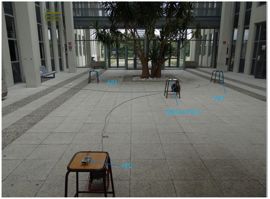
Figure 1.
Measurement scenario.
To establish a practical channel model in this hall, many measurements have been performed at different positions. The distances between the transmitter (mobile device) to receiver (one of the three AP), are from 1 m to 10 m. In the testing, we find that the received RSSI value is always −10dBm when the distance is not more than 1 m. Therefore, in the measurement, we start the distance form 1 m. To obtain different samples of RSSI for one position, in the measurement, we can adopt the following procedures. First, we change mobile point position to a very small distance. This changing distance is so small that it can be negligible for localization. Second, we can put some obstacles in the measurement region to make the environment more complicated. Third, a person is moving in the localization region when the measurement is being done. These measurement means will change the transmission environments between signal receiver and sender, and many fluctuating RSSI values for one position will be collected. The averaged RSSI is calculated from many RSSI values based on different distances. For one same position, we change the mobile position a very small distance, or a person is walking in this region when the measurements are being performed. In this manner, 30 different RSSI values will be collected for one position. Then, we calculate the average RSSI from 30 RSSI values. For example, at a distance of 5 m, the position of the mobile point is changed by a very small distance 30 times, and 30 different RSSI values are collected for calculating the averaged RSSI value.
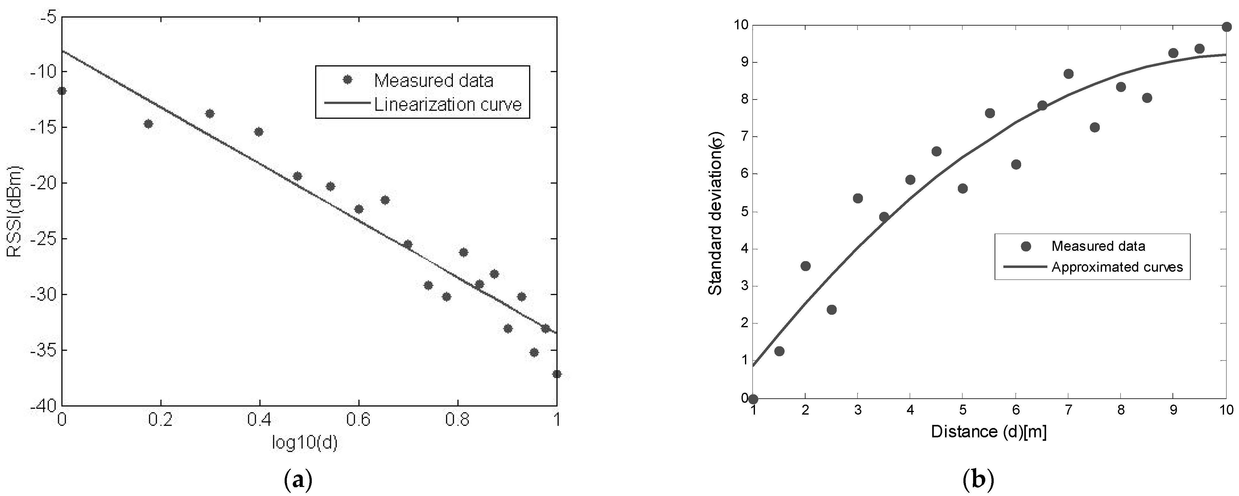
Figure 2a presents the measured averaged RSSI as function of the distance. As expected, we can find that the RSSI value decreases with the distance. From these results we can deduce the following channel model:
with a zero-mean random variable with standard deviation .

Figure 2.
(a) Relationship of measured RSSI values and distance. (b) Relationship of the noise standard deviation and distance for measured data.
Comparing Equations (1) and (5), we can find that the parameter is equal to 2.27135. Parameter denotes the complexity of the environment. The larger the value of , the more complex the environment. In Equation (5), we also need to know the To determine the relationship between the variance of the noise and distance, based on the RSSI values that have been acquired as before and the standard deviation of the noise, we use:
where is defined in Equation (4).
The obtained results are shown in Figure 2b. From the experimental results, the standard deviation of the noise, in terms of the distance from 1 to 10 m, can be expressed as:
The variance model defined by Equation (7) is specific to our measurement condition but indicates that the RSSI variance tends to increase with distance, which has already been observed in some work [27]. The relationship of the noise variance and distance depends on the environment size and complexity. It is worth noting that this channel model expressed by Equations (5) and (7) is specific to the measurement environment and based on the distance below 10 m. It needs to be emphasized that this channel model is only suitable for the distance below 10 m and cannot be generalized for larger distances. In our work, we consider the distance below 10 m. In the test, we also collected data from larger distances, such as above 10 m. We found that large distances will give large variances. We also found that large distances will also give large localization errors. Therefore, in our work, we only consider the distance below 10 m to achieve a better localization performance. We did measurements on the condition that the distance is within 10 m and analyzed these measurements. If we want do localization in a larger region, we can subdivide this region into some smaller ones by adding more anchors into it or we need to do measurements based on larger distances, such as 15 m, 20 m and so on to construct the RSSI model.
2.1.3. Simulated Channel Model
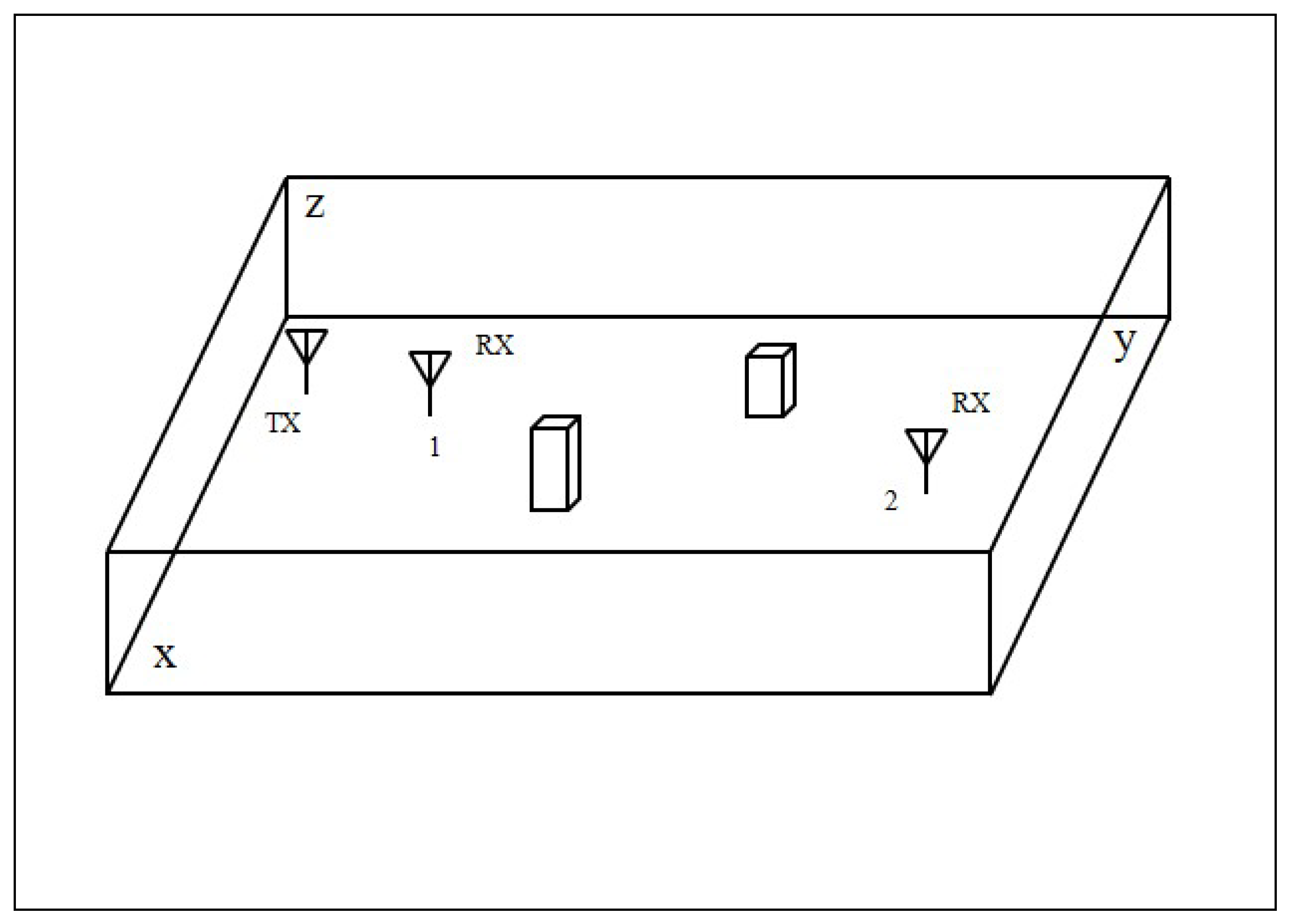
The previous subsection presents the channel model based on measured RSSI data, which are provided by a practical testing system. The results show that the RSSI value decreases with increased distance. The noise variance increases with increased distance. To confirm this trend, we have designed a ray-tracing system whose simulation scenario is shown in Figure 3. Simulation is done using this ray-tracing system for an indoor environment similar to the experimental environment. We simulate a workshop for the indoor environment. Signal sending and receiving occur within this workshop. In this ray-tracing system, four cases are considered to define different environment conditions. Two cases have obstacles in an indoor workshop and another two cases have no obstacles in them. As illustrated in this simulation scenario, there is a simulated workshop with two obstacles in it. A transmitter denoted by TX sends a signal to a mobile receiver denoted by RX, which moves from position 1 to position 2. In the simulation, the averaged RSSI value is calculated based on these simulated data. The relationships between the distance and standard deviation of noise for four cases are observed.
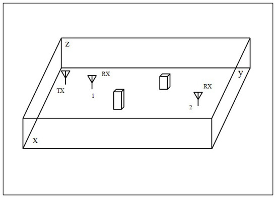
Figure 3.
Simulation scenario of ray-tracing system.
In the first two cases, we observe the relationship between the RSSI values and distance with no obstacle in the room. The size of workshop for case 1 and 2 are different. In the third and fourth cases, we change the room size or put two obstacles in it. The detailed information for these four cases is illustrated in Table 1. In case 1 and case 3, the length, width and height of the workshop are set to 15 m, 8 m and 5 m. In case 2 and case 4, the length, width and height of the workshop are set to 30 m, 10 m and 5.5 m. Meanwhile, there is no obstacle in the workshop for case 1 and case 2. Two obstacles, as shown in Figure 3, are placed between the sender and receiver and do not block the signal sender and receiver completely in the workshop for case 3 and case 4. Moreover, we set the transmission power at −100 dBm consistently for four cases. Similarly, the frequency is assigned as 2465 MHz for all cases. In the ray-tracing work, we consider 3 reflections for case 1 and 2, and 5 reflections for case 3 and 4. To simplify this ray-tracing process, we do not consider signal scattering and others. As for attenuations caused by reflections, we set reflection attenuation factor as 0.25. That is to say that the reflected signal power will be decreased to 25% of that of incident signal. We use free space path loss model in this process to calculate signal attenuation. In this simulation, we suppose the receiver has a better sensitivity, which can receive very low-power signal, far below −100 dBm.

Table 1.
Environment information for four cases.
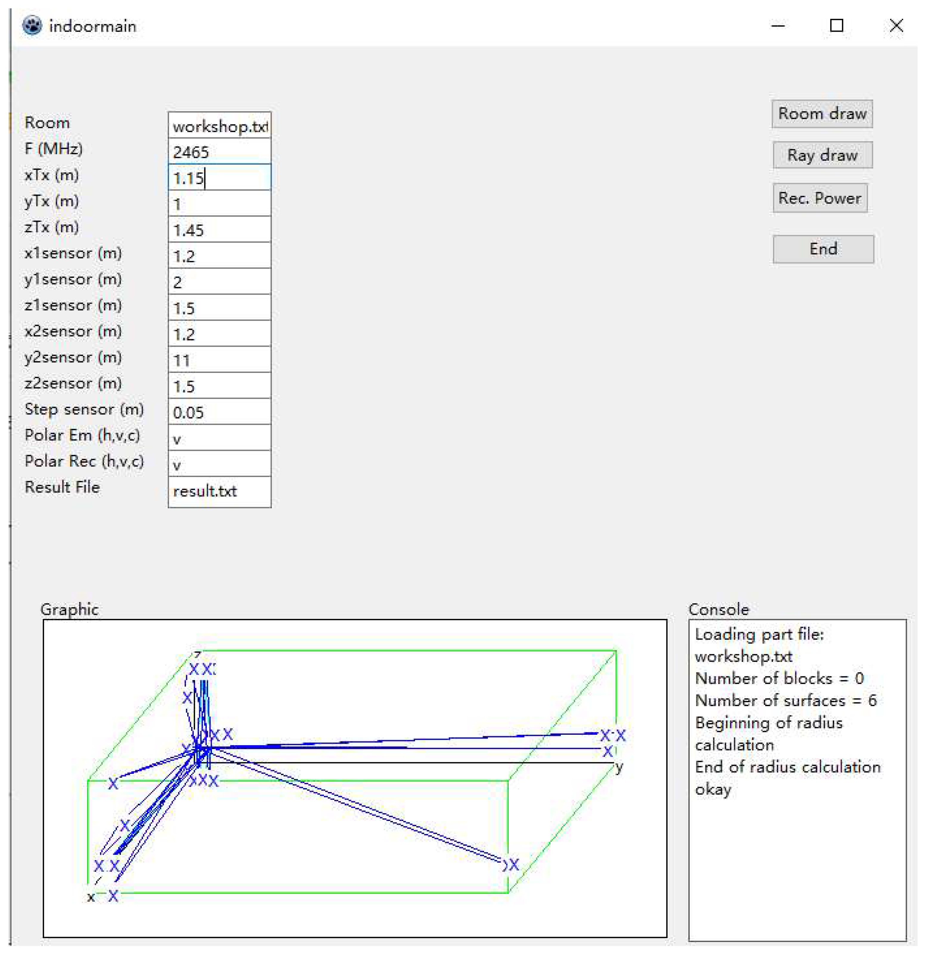
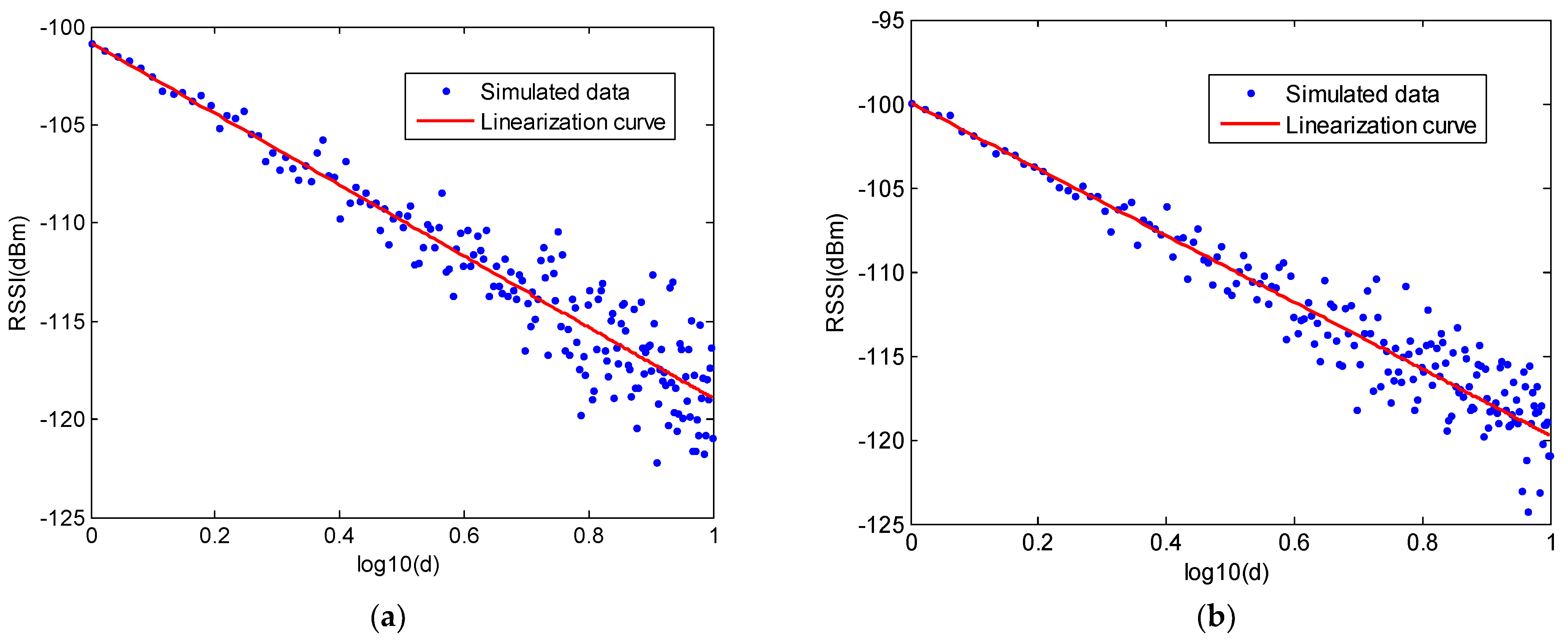
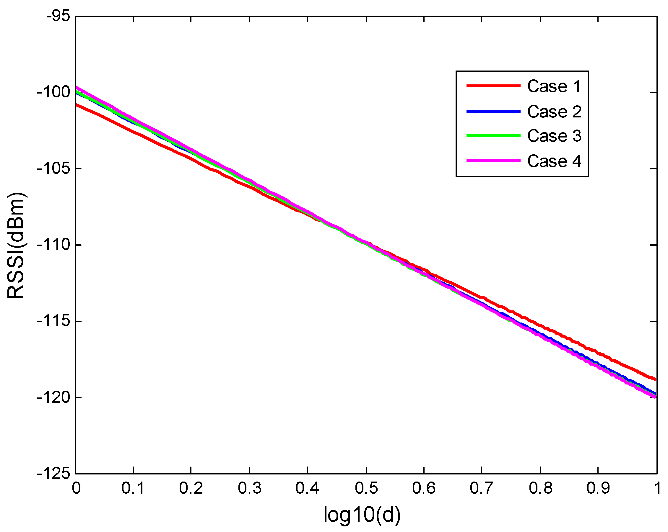
The interface of ray-tracing system is shown in Figure 4. At the top of this interface, we can set some parameters in this simulator. Specification of the workshop is regulated by a txt file and will be imported into simulator. This txt file will define the workshop size and the number of obstacles. The positions of two obstacles are also defined in this txt file. The position of signal sender and receiver can be set. Furthermore, other parameters, such as frequency, step and so on also can be set in this simulator. For four cases, the position signal sender TX and position of RX 1, 2 are set to be (1.15, 1, 1.45), (1.2, 2, 1.5), (1.2, 11, 1.5) respectively. The step sensor is set as 0.05, which denotes the moving step from position 1 to 2. We can draw the room and ray path by the buttons at the top right of the interface. The simulated RSSI values will be saved in a txt file. In the simulation, for one position, 30 different RSSI values are measured, and 180 positions are considered by changing the distance from 1 m to 10 m with interval of 0.05 m. Therefore, in this simulator, we also consider the distance to be below 10 m to construct the channel model in line with the measurement system. Similarly, in a similar manner to the real RSSI collection from the previous system, simulated RSSI values are acquired from this ray-tracing system. Then, the averaged RSSI are calculated for one distance and the relationship between the distance and RSSI are plotted for four cases. These results are shown in Figure 5a–d. Moreover, the linear approximations for the four cases are plotted in Figure 6. Based on these simulated RSSI data, the values of parameters and for all cases are estimated and given in Table 2.
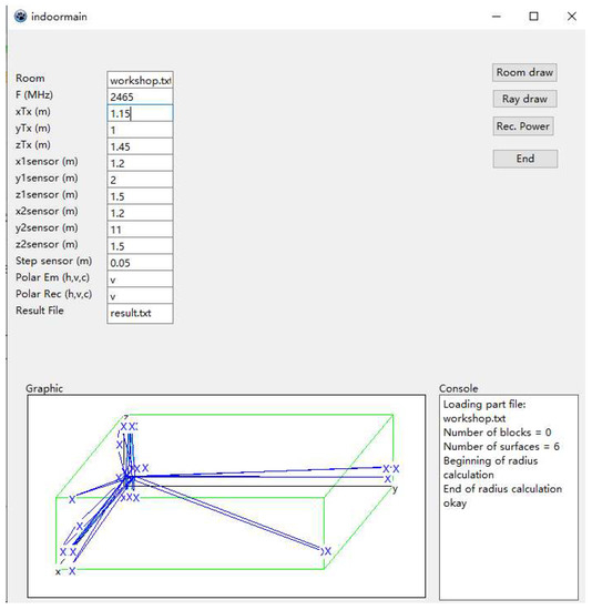
Figure 4.
Interface of ray-tracing system.
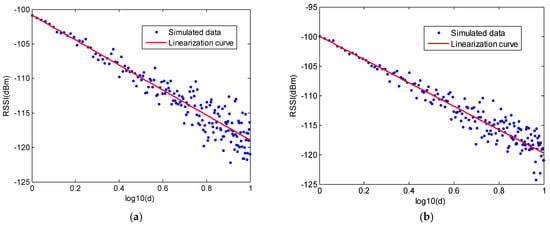
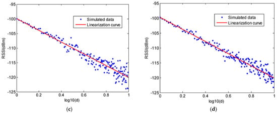
Figure 5.
(a) Relationship of the simulated RSSI values and distance for case 1; (b) Relationship of the simulated RSSI values and distance for case 2; (c) Relationship of the simulated RSSI values and distance for case 3; (d) Relationship of the simulated RSSI values and distance for case 4.
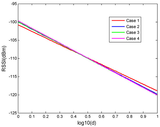
Figure 6.
Comparison of the linearization curves for four cases.

Table 2.
Different parameter values for four cases.
From these results, we can compare the channel model parameters for four cases. In the first and second cases, there is no obstacle in the workshop. In the second case, we enlarge the room size. By comparing the parameters of case 1 and 2, we can find that value increases from −100.20 to −99.99, which represents a very small evolution. Similarly, value decreases from 1.95 to 1.99. This is because the reflected signal strength weakens when the room size is enlarged. It needs to be explained that the values in Table 2 are based on the fitting curves of the simulated data. We can find that the A value is larger than the transmitting power −100 dBm. This does not mean that the RSSI values will be larger than −100 dBm. All the simulated RSSI values are below −100 dBm. In the channel model, value denotes the signal attenuation. In a more complex environment, signal will attenuate quickly, which will involve a larger value. As shown in Figure 5, for all cases, RSSI values decrease with the increased distance, which is in line with the change tendency of the measured RSSI from the testing system. For four cases, as shown in Figure 6, they give different attenuation factors depending on different transmitting environments.
In the third and fourth cases, we put two obstacles in the room, as shown in Figure 3. It indicates that increases when obstacles are put in the measurement space. This is because the signal attenuates when there are obstacles between the transmitter and receiver. Moreover, all values based on measured data are larger than that based on the simulated data. The reason for this difference is first that the simulation scenario is simpler than the real measurement environment, and secondly that the simulator simplifies the physical phenomena of propagation.
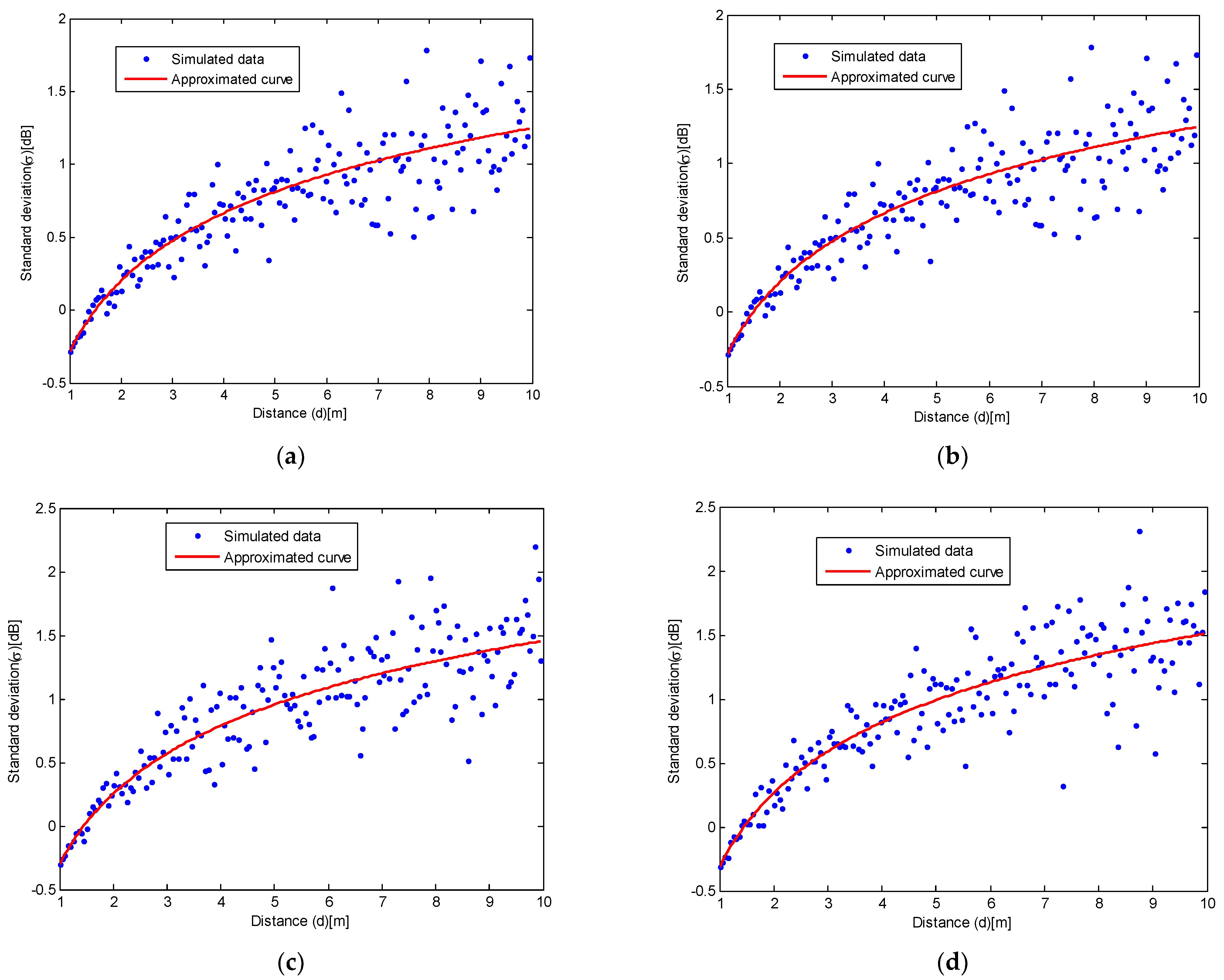
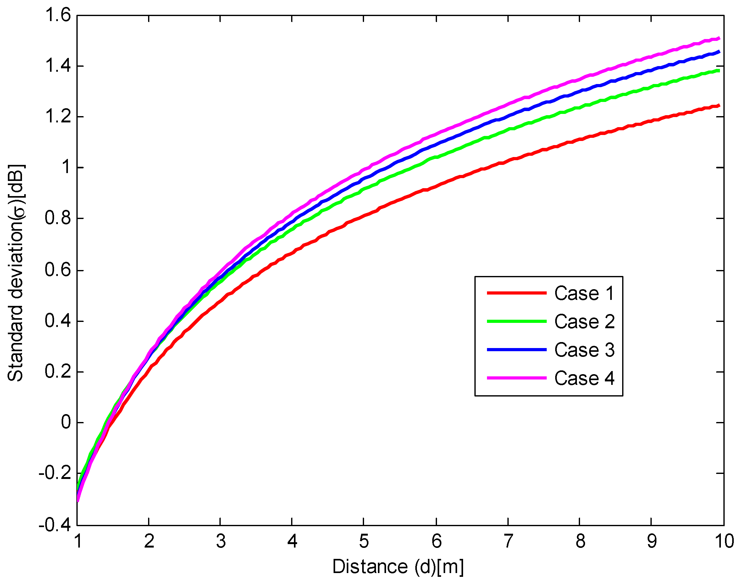
Similar to the calculation means on measured RSSI data, the relationship of standard deviation of noise and distance based on the simulated RSSI also be drawn. The relationships between the standard deviation of noise and distance for four cases are plotted in Figure 7a–d. Moreover, comparison of the relationship between the noise standard deviation and distance based on simulated data for four cases is plotted in Figure 8. The standard deviation of the noise, in terms of the distance from 1 to 10 m, can be expressed by Equation (8) for case 1, Equation (9) for case 2, Equation (10) for case 3 and Equation (11) for case 4, respectively.
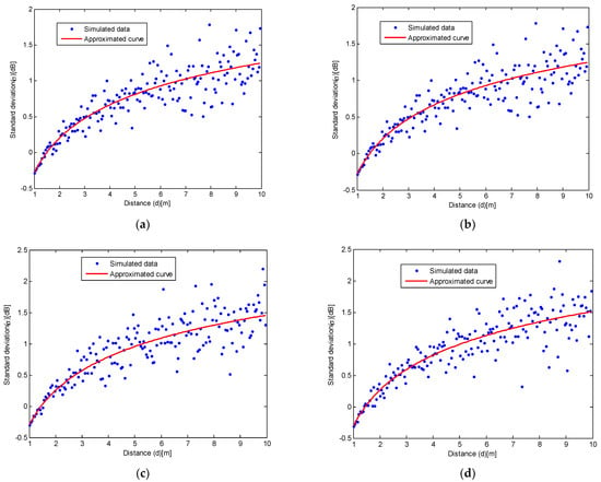
Figure 7.
(a) Relationship of the noise standard deviation and distance based on simulated data for case 1; (b) Relationship of the noise standard deviation and distance based on simulated data for case 2; (c) Relationship of the noise standard deviation and distance based on simulated data for case 3; (d) Relationship of the noise standard deviation and distance based on simulated data for case 4.

Figure 8.
Comparison of relationship between the noise standard deviation and distance based on simulated data for four cases.
From the above analysis on the simulated RSSI data, it can be observed that the real and simulated data have a similar tendency in terms of the relationship between the noise standard deviation and distance. The noise standard deviation increases with distance when the distance is restricted below 10 m. However, due to the complex environment, the standard deviation based on real data is larger than the simulated data. These channel model experiment results show that a more complex signal transmitting environment will give a larger attenuation factor and a larger noise, which is consistent with the theoretical channel model.
2.2. Localization Algorithms
The previous section has shown that the relationship between the RSSI value and distance can be written as:
where and are channel parameters whose values change with the environment and is a noise whose variance is also largely variable.
Therefore, the RSSI is not reliable for deducing distance. The objective of this section is to propose and evaluate some localization algorithms by taking into account the low accuracy of distances deduced from RSSI measurements. Based on the principle of multilateration and distance estimation formula, we analyze the factors affecting positioning performance, find the law of error, verify the relationship between distance and error, deduce weighted factors, and establish a novel position optimization equation. Based on the above achievements, an approach named weighted three minimum distances method (WTM) is proposed. Using the testbed described in the last section, an experimental channel model is deduced to verify the performance of the proposed algorithm under realistic conditions. Simulations will be done to show that the proposed method can achieve better accuracy. In the following subsections, the proposed localization algorithm is detailed and performance comparisons are presented.
2.2.1. Distance Estimation from RSSI
The proposed algorithm is based on the distance estimated from RSSI. Therefore, the first step of the study is to define a method to do this estimation and to evaluate the distance accuracy.
Suppose that the distance estimation is based on M samples of , which represents the th RSSI sample measured by the th anchor node. To achieve a good performance, the mean value of is used to obtain the distance estimate:
where , the mean RSSI value measured by the th anchor, is given by:
It should be noticed that the mean value can be replaced by the median value in practical situations, with the advantage that the median value is less sensitive to outliers. In our model, because the is Gaussian distributed, the mean value is equal to the median value.
Using a channel model defined by Equation (2) and substituting Equation (14) into Equation (13), we can deduce the estimated distance as:
If the noise is small or the number of samples M is large, the estimated can be approximated by:
Then the measurement error can be evaluated by the following additive noise:
Its variance is given by:
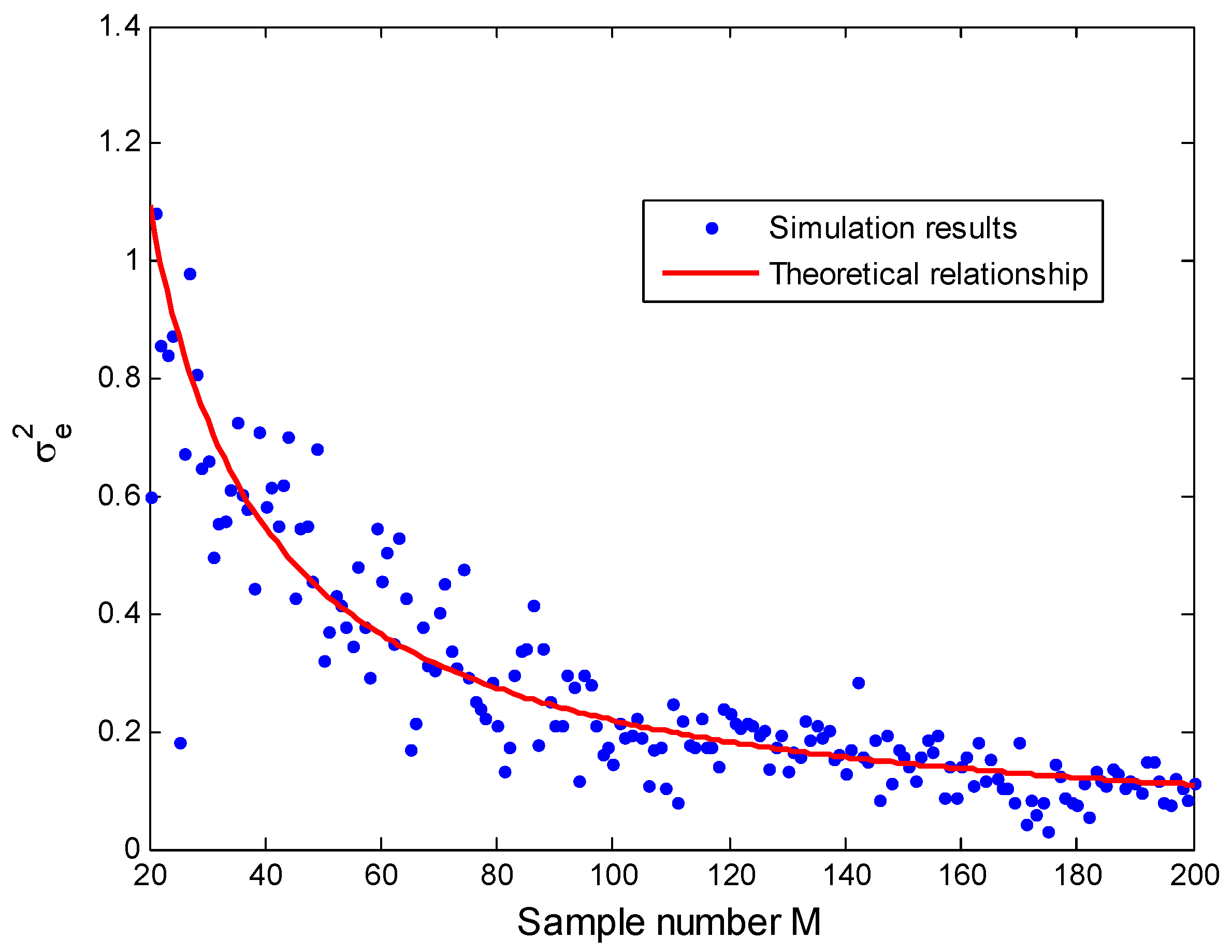
To confirm this theoretical derivation, simulations are performed to observe the relationship between the distance variance and the sample number M. In Figure 9, a distance value is given to be 5 and the relationship between the distance variance and the sample number is plotted. These results indicate that the simulation results match well with the deduced expression although there exists error caused by noise. With the increase of the sample number M, the error between the measured distance variance and theoretical value becomes smaller.
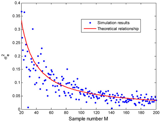
Figure 9.
Relationship between and M for .
When the distance value is set to 8, a similar result can be obtained which is illustrated in Figure 10. As expected, the distance variance becomes larger when the distance increases. From Equation (18) we can deduce that the variance of the estimated distance depends on the distance and on the measurement noise variance. From the previous study, we also know that the noise variance increases with the distance. It is clear that a large distance corresponds to a stronger estimation variance, giving a less precise estimation of the distance. Analysis results of the distance estimation error, expressed by Equation (18), provides some guidance to reduce localization error, such as using the smallest distance from the unknown node to anchor nodes or increasing the sample number M. This error analysis conclusion will be used to design a novel algorithm in our work.
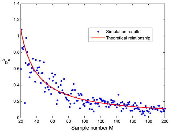
Figure 10.
Relationship between and M for .
2.2.2. Multilateration
The multilateration algorithm is a basic positioning method, widely used in many localization systems [28,29]. In this algorithm, at least three anchor nodes are needed for two-dimensional localization. The position of the anchor nodes is assumed to be known. The relationship between the unknown node position and N anchor nodes positions can be expressed as:
where is the coordinates of the reference or unknown nodes, , , , and are the coordinates of the N anchors.
In ideal conditions, in the absence of fading, noise and channel model error, the above equations represent N circles that will intersect at only one position. This intersected point is the actual position. Unfortunately, in practical conditions, the N circles do not intersect at one position due to fading and noise impacts. For example, when the number of anchors is equal to 3, Figure 11a,b show the three circles under ideal conditions and under real conditions. In the case of real conditions, we need to find the most likely position in other ways.
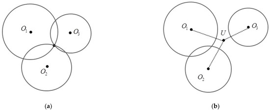
Figure 11.
(a) Location relationships of three circles in ideal conditions; (b) Location relationships of three circles in real conditions.
2.2.3. Proposed Method
To approximate the most likely position, nonlinear least square (NLS) has been proposed. The nonlinear optimization problem can be solved using the sequence quadratic programming algorithm [30,31]. In this paper, we propose a novel method based on NLS, called WTM. For this proposed method, the objective minimization function is modified, and the best position is given by:
where N is the number of anchors, is the estimated position, is the coordinates of the kth anchor and the estimated distance from the averaged RSSI value at the kth anchor. We introduce a weight used for each estimated distance .
The weights are introduced to deal with the fact that the distance estimation variance increases with the distance. The weight values differ with different estimated distances. For proposed WTM, first, the n (3 ≤ n ≤ N) smallest estimated distances are selected from the N available distances. Then, different weight values are assigned for the n selected distances. For example, when n equal to 3, the three smallest estimated distances are selected from N available distances, and when n is equal to N, all the estimated distances are selected from N available distances. The value n can be adapted and can vary from 3 to N in the proposed algorithm. Therefore, the weight values are assigned as:
From the above study, we know that the noise variance increases with the distance. It is clear that a large distance corresponds to a stronger estimation variance, giving a less precise estimation of the distance. According to Equation (18), we assigned different weighted values to different distances. Therefore, using the weight value assigned in Equation (23), the uncertainty of the measured distances can be taken into account in the objective function. Considering both Equations (18) and (20), and for reducing the computation complexity, we set the power exponent in the weight value as 4. In practice, the estimated standard deviation in Equation (23) is estimated from Equation (6).
3. Experiment and Analysis
To evaluate the proposed localization algorithm, the experiment and analysis will be done in this section. In the performance comparison, we choose three existing algorithms: NLS, LM, and SDP, to compare. For WTM, two cases: n = 3 and n = N are considered in the performance comparison. Both simulated and measured RSSI data will be used to verify the performance of NLS, LM, SDP and WTM, which will be detailed in the following sections.
3.1. Simulated Data Verfication
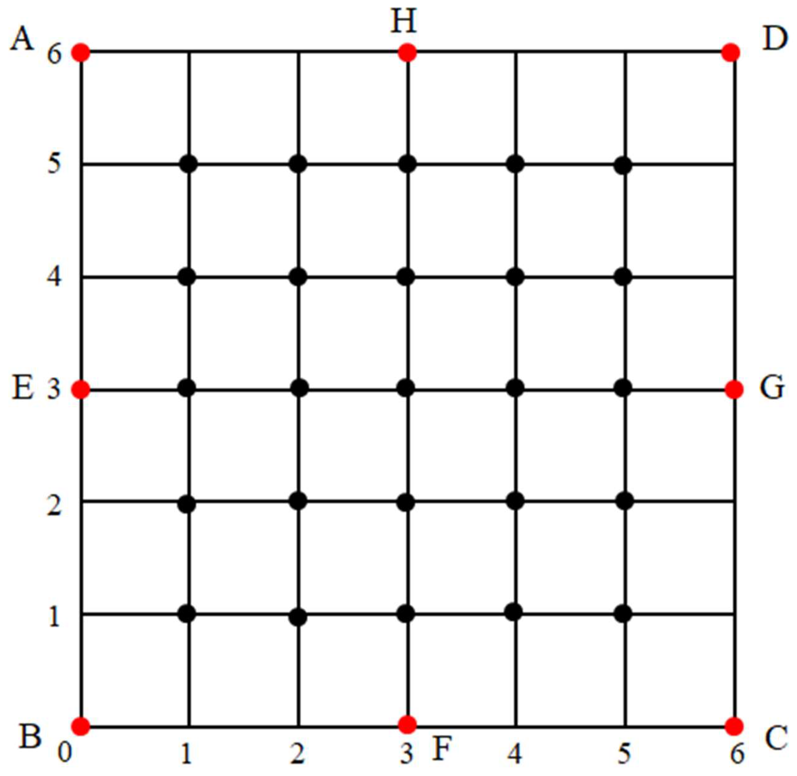
After acquiring the channel model from the experimental data, the whole localization process can be evaluated in a given region. As shown in Figure 12, eight anchor nodes which are denoted by red dots are set in the predefined positions with coordinates A(0,6), B(0,0), C(6,0), D(6,6), E(0,3), F(3,0), G(6,3), H(3,6). In the coordinate scale, 1 denotes 1 m. When the number of anchors is three, the anchor nodes are located at A, B, and C. When this number is four, the fourth node is located at D. In a similar letter order, more anchors positions can be determined. When the anchor number is eight, the eight anchor nodes are deployed regularly on the edge of this region.
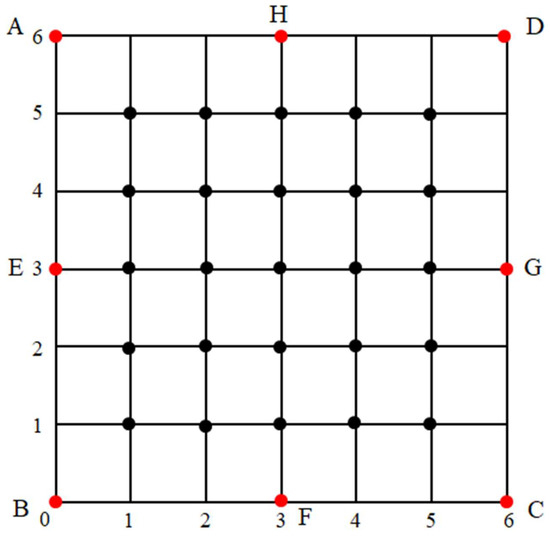
Figure 12.
Grid defining the intersection positions and anchor nodes positions.
In the simulation, the unknown node position is randomly selected from the intersection points of the grid, which is denoted by black dots, as shown in Figure 12. We define this localization region to simulate a room. We will locate the anchor nodes on the wall of the room. In this indoor localization region, all the moving objects within this room will be surrounded by all anchor nodes. Based on this application scenario, in our work, we only consider the localization problem inside an area formed by the anchors. Then, for each selected position, we calculate the root mean square error (RMSE) [32] value defined as:
where is the real selected position. is the position estimated by the compared localization methods. T is the number of randomly chosen positions. In the simulation, T is equal to 500.
To increase the accuracy of the localization methods, we need to acquire many RSSI values for the proposed algorithms. Using simulation results based on the experimental channel model, M different samples of RSSI are acquired for each selected position. Then the averaged RSSI value is calculated from M sampled values and the coordinates of the position are estimated. In this simulation, in line with the sample number in the channel model, the number of samples M is equal to 30. In the practical application, a higher sample number M will give higher localization accuracy. If we increase this value, the accuracy of the algorithms will increase. Meanwhile, collecting RSSI data will consume time. A large sample number will increase time delay. We need to make a tradeoff between localization time and accuracy. In our work, we choose a moderate sample number of 30. In the following sections, we will present the comparison of localization performance in terms of accuracy and time overhead for the four compared localization algorithms.
3.1.1. Localization Accuracy
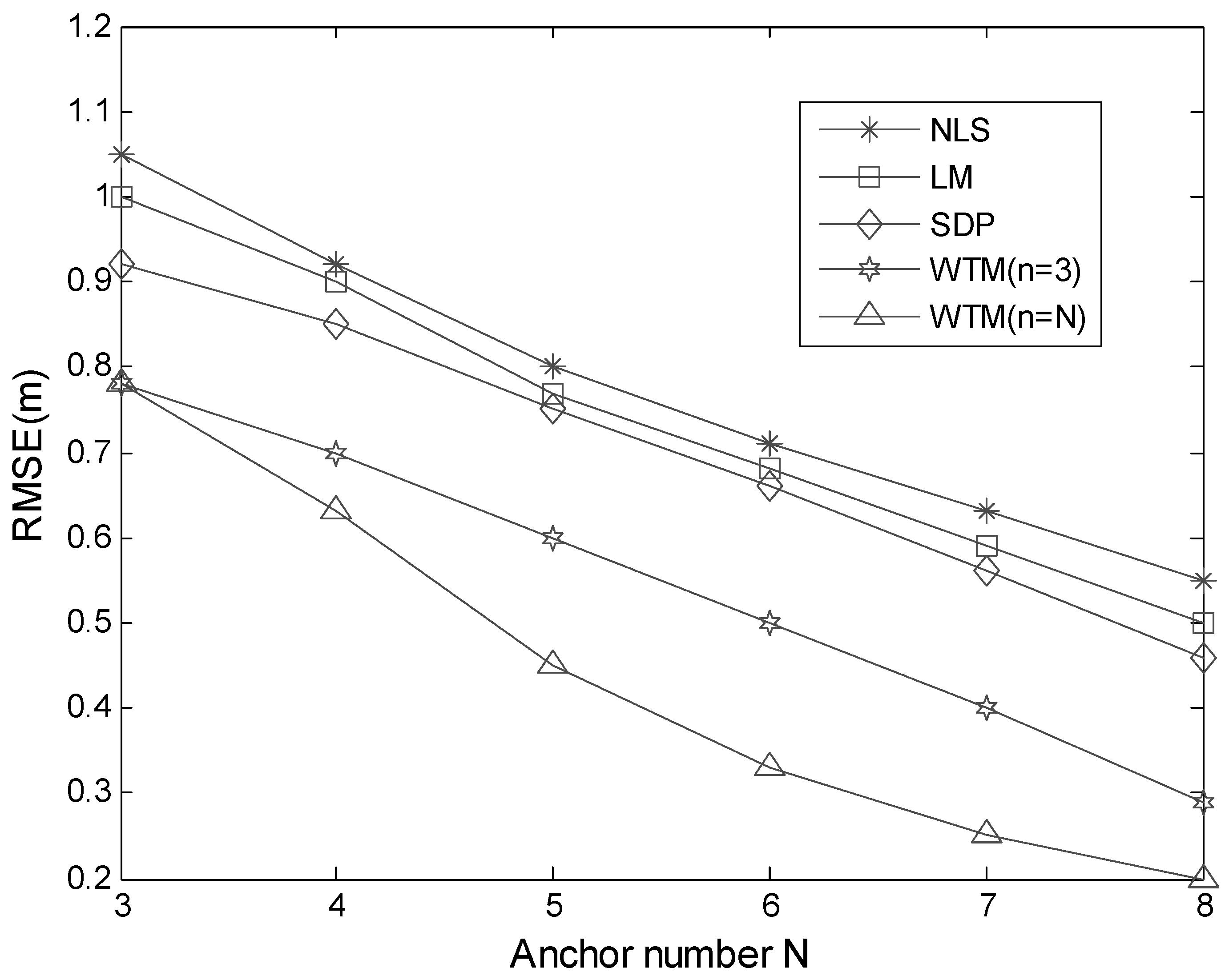
In this special simulation scenario, the possible searched region is defined by the square area limited by A, B, C and D. From Equation (24), we know that a smaller RMSE value indicates a higher accuracy. As illustrated in Figure 13, the changing RMSE tendencies for the four compared algorithms based on different anchor number are plotted. Overall, among these four algorithms, WTM (n = N) gives the highest localization accuracy and NLS gives the lowest. Since the proposed algorithms are based on an improved NLS, we can see that the improvement in the term of accuracy is obvious. When the number of anchors is 3, WTM (n = 3) and WTM (n = N) are equivalent, so the accuracy of them is identical. When the anchor number increases from 4 to 8, we can find that WTM (n = N) is better than WTM (n = 3). When the number of anchors is 3, 4, 5, 6, 7 and 8, the RMSE value of SDP is smaller than that of LM and NLS, which indicates that the accuracy of the SDP is superior to that of NLS and LM. LM is better than NLS in terms of localization accuracy. WTM gives higher localization accuracy than SDP, LM and NLS. Moreover, with respect to all algorithms, when the anchor number increases, the localization accuracy will increase. This indicates that employing more anchor nodes will increases accuracy. From all these results, we select RMSE values for four algorithms based on eight anchors to do quantitative analysis. When the anchor number is raised to eight, the RMSE values for NLS, LM, SDP, WTM (n = 3) and WTM (n = N) are 0.55, 0.50, 0.46, 0.29 and 0.20, respectively. From these results, we can see that WTM (n = N) has about 64% improvement with respect to NLS in terms of localization, and WTM (n = 3) has about 60% improvement. Compared with the SDP, WTM (n = N) has about 57% improvement on accuracy and WTM (n = 3) has about 46% improvement. Among all these algorithms, the proposed WTM (n = 3) and WTM (n = N) have better performance in the term of localization accuracy.
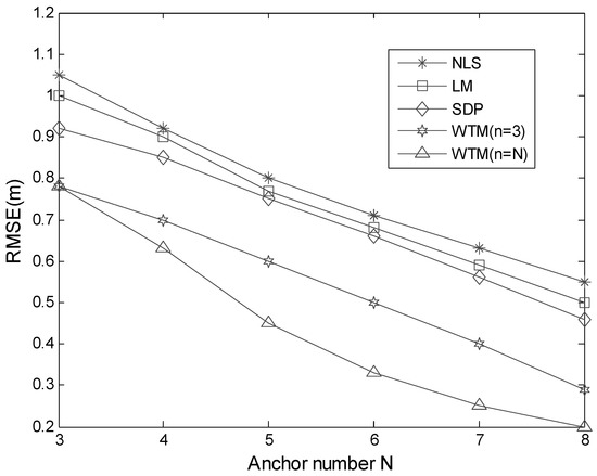
Figure 13.
Localization accuracy for NLS, LM, SDP and WTM based on simulated RSSI data.
3.1.2. Time Overhead
We also compared the calculated time for the four algorithms. The simulation times (ST) for each method implemented in MATLAB software on a computer with processor unit (CPU) of 2.6 GHz and 16 GB of RAM are observed. The time cost of each positioning process for the four algorithms is shown in Table 3. From these calculation time results, we can see that the influence of the number of anchors on simulation time is negligible. This indicates that the calculation time is mainly comprised of optimal point searching time. The calculation times for one single localization process of NLS and LM are 25 ms and 42 ms, respectively. The calculation time is almost the same for SDP, WTM (n = 3) and WTM (n = N), which is 58 ms. These results show that the proposed WTM (n = 3) and WTM (n = N) will consume more calculation time. Compared with NLS, the calculation time of WTM (n = 3) and WTM (n = N) are increased by 132%. Therefore, WTM (n = 3) and WTM (n = N) will involve a larger time overhead. In the view of this situation, we need to perform the localization process on the remote computing server to speed up the localization process. In practical application, collecting RSSI data from anchor nodes will consume time. Therefore, the whole localization time is composed of RSSI collecting time and calculation time. Compared with calculation time, RSSI collecting time is far larger in the localization process. When the anchor nodes number is 3, the WTM (n = 3) and WTM (n = N) are the same. When the anchor number is more than 3, the localization accuracy of WTM (n = N) is better than the WTM (n = 3). More anchor node will consume more RSSI collecting time. There is always a contradiction between time consumption and localization accuracy. If we want to achieve higher accuracy, we can choose WTM (n = N). On the contrary, the WTM (n = 3) method will consume less localization time than WTM (n = N) in the real application. Furthermore, we can adjust n values form 3 to N to achieve a tradeoff between accuracy and localization time in the practical application.

Table 3.
Simulation time for one localization process in milliseconds.
3.2. Measured Data Verfication
In our work, we also did performance comparison based on measured RSSI values form the testing system. Since there are only three anchor nodes in the experimental positioning system, we can only verify when the number of anchor nodes is equal to 3 for the localization algorithms based on measured data. In the experimental scenario shown in Figure 1, we deploy three anchor nodes at points A, B, and C in an indoor environment. In this experimental testing hall, the coordinates of the three points A, B and C are (0, 6), (0, 0), and (6, 0) respectively. In the RSSI data collection, we selected three points (3, 2), (1, 5), and (5, 5) to measure and collect the RSSI data. The number of RSSI data collected at each point is equal to 30. After collecting the RSSI data, we estimated the distance to the three anchor nodes and calculated the position for these three points by the four positioning algorithms. Finally, we calculated the value of RSME obtained at three points, and the results are shown in Table 4.

Table 4.
Localization results for NLS, LM, SDP and WTM based on measured RSSI data for three selected points.
From the RMSE results of the four algorithms obtained from the measurement data, similar to the results based on simulated data, WTM (n = 3) and WTM (n = N) will give the best localization accuracy. The main difference is that the RMSE values of each algorithm based on the measured data is larger than the RMSE values based on simulated data. This is because in the real measurement environment, due to changes in the environment, the collected RSSI data have greater irregularities, so the positioning accuracy is lower than the simulated data. For the three selected points (3, 2), (1, 5), and (5, 5), their localization accuracy have slight differences. The localization accuracy of point (3, 2) is slightly better than (1, 5), and (5, 5), which is caused by the anchor node deployment. From the RMSE values given by point (5, 5), we can see that WTM (n = 3) and WTM (n = N) give an identical value 0.95. Compared with NLS and SDP, the accuracy improvement is about 43% and 28% by WTM (n = 3) and WTM (n = N). These experimental results indicate that the proposed WTM (n = 3) and WTM (n = N) will give better performance in terms of localization accuracy.
4. Conclusions
In this paper, an approach called WTM based on multilateration is proposed to deal with the poor accuracy of distances estimated from RSSI values. Averaged RSSI is calculated for distance estimation, and the multilateration is adopted to estimate the position. Based on practical data acquired from a real localization system, an experimental channel model is constructed to evaluate the proposed algorithms. Distance estimation error is analyzed, and the weight factors are derived from the RSSI channel model. Based on the analysis result of the distance estimation error, a novel algorithm is proposed. The measured RSSI data are also used to evaluate the localization performance for the compared algorithms. Compared with the existing NLS, LM and SDP algorithms, the proposed localization algorithm exhibits better performance in terms of localization accuracy.
Author Contributions
Methodology and Conceptualization, J.D. and C.Y.; Writing—original draft and Data curation, J.D. and M.Y.; Software and Visualization, C.Y. and T.M.; Formal analysis, Validation and Writing—review and editing, M.Y. and T.M. All authors have read and agreed to the published version of the manuscript.
Funding
This research was funded by the Science and Technology Foundation for Youths of Gansu Province, China (Grant No. 20JR10RA185).
Conflicts of Interest
The authors declare no conflict of interest. The funders had no role in the design of the study; in the collection, analyses, or interpretation of data; in the writing of the manuscript, or in the decision to publish the results.
Abbreviations
The following abbreviations are used in this manuscript:
| WSNs | wireless sensor networks |
| TOA | time of arrival |
| TDOA | time difference of arrival |
| RSSI | received signal strength indicator |
| AOA | angles of arrival |
| ML | maximum likelihood |
| LLS | linear least squares |
| NLS | nonlinear least squares |
| LM | Levenberg–Marquardt algorithm |
| SDP | semidefinite programming |
| WLS | weighed least squares |
| WTM | weighted three minimum distances method |
| AP | access points |
| RMSE | root mean square error |
References
- Behera, A.P.; Singh, A.; Verma, S.; Kumar, M. Manifold Learning with Localized Procrustes Analysis Based WSN Localization. IEEE Sens. Lett. 2020, 4, 1–4. [Google Scholar] [CrossRef]
- Darakeh, F.; Mohammad-Khani, G.-R.; Azmi, P. DCRL-WSN: A distributed cooperative and range-free localization algorithm for WSNs. AEU-Int. J. Electron. Commun. 2018, 93, 289–295. [Google Scholar] [CrossRef]
- Poulose, A.; Han, D.S. Hybrid Deep Learning Model Based Indoor Positioning Using Wi-Fi RSSI Heat Maps for Autonomous Applications. Electronics 2021, 10, 2. [Google Scholar] [CrossRef]
- Singh, S.P.; Sharma, S.C. A PSO Based Improved Localization Algorithm for Wireless Sensor Network. Wirel. Pers. Commun. 2018, 98, 487–503. [Google Scholar] [CrossRef]
- Pandey, O.J.; Gautam, V.; Jha, S.; Shukla, M.K.; Hegde, R.M. Time Synchronized Node Localization Using Optimal H-Node Allocation in a Small World WSN. IEEE Commun. Lett. 2020, 24, 2579–2583. [Google Scholar] [CrossRef]
- Pandey, O.J.; Mahajan, A.; Hegde, R.M. Joint Localization and Data Gathering Over a Small-World WSN with Optimal Data MULE Allocation. IEEE Trans. Veh. Technol. 2018, 67, 6518–6532. [Google Scholar] [CrossRef]
- Shieh, C.-S.; Sai, V.-O.; Lee, T.-F.; Le, Q.-D.; Lin, Y.-C.; Nguyen, T.-T. Node Localization in WSN using Heuristic Optimization Approaches. J. Netw. Intell. 2017, 2, 275–286. [Google Scholar]
- Kumar, S.; Kumar, S.; Batra, N. Optimized Distance Range Free Localization Algorithm for WSN. Wirel. Pers. Commun. 2021, 117, 1879–1907. [Google Scholar] [CrossRef]
- Zhu, H.; Luo, M. Hybrid robust sequential fusion estimation for WSN-assisted moving-target localization with sensor-node-position uncertainty. IEEE Trans. Instrum. Meas. 2020, 69, 6499–6508. [Google Scholar] [CrossRef]
- Dong, S.; Zhang, X.-G.; Zhou, W.-G. A Security Localization Algorithm Based on DV-Hop Against Sybil Attack in Wireless Sensor Networks. J. Electr. Eng. Technol. 2020, 15, 919–926. [Google Scholar] [CrossRef]
- Singh, S.P.; Sharma, S.C. Implementation of a PSO Based Improved Localization Algorithm for Wireless Sensor Networks. IETE J. Res. 2019, 65, 502–514. [Google Scholar] [CrossRef]
- Parras, J.; Zazo, S.; Pérez-Álvarez, I.A.; González, J.L.S. Model Free Localization with Deep Neural Architectures by Means of an Underwater WSN. Sensors 2019, 19, 3530. [Google Scholar] [CrossRef] [PubMed] [Green Version]
- Haider, A.; Wei, Y.; Liu, S.; Hwang, S.-H. Pre- and Post-Processing Algorithms with Deep Learning Classifier for Wi-Fi Fingerprint-Based Indoor Positioning. Electronics 2019, 8, 195. [Google Scholar] [CrossRef] [Green Version]
- Singh, P.; Mittal, N. An efficient localization approach to locate sensor nodes in 3D wireless sensor networks using adaptive flower pollination algorithm. Wirel. Netw. 2021, 27, 1999–2014. [Google Scholar] [CrossRef]
- Schlupkothen, S.; Prasse, B.; Ascheid, G. Backtracking-based dynamic programming for resolving transmit ambiguities in WSN localization. EURASIP J. Adv. Signal Process. 2018, 2018, 1–26. [Google Scholar] [CrossRef]
- Cheng, L.; Li, Y.; Xue, M.; Wang, Y. An Indoor Localization Algorithm Based on Modified Joint Probabilistic Data Association for Wireless Sensor Network. IEEE Trans. Ind. Inform. 2020, 17, 63–72. [Google Scholar] [CrossRef]
- Prashar, D.; Jyoti, K. Distance Error Correction Based Hop Localization Algorithm for Wireless Sensor Network. Wirel. Pers. Commun. 2019, 106, 1465–1488. [Google Scholar] [CrossRef]
- Chelouah, L.; Semchedine, F.; Bouallouche-Medjkoune, L. Localization protocols for mobile wireless sensor networks: A survey. Comput. Electr. Eng. 2018, 71, 733–751. [Google Scholar] [CrossRef]
- Meng, H.; Yuan, F.; Yan, T.; Zeng, M. Indoor Positioning of RBF Neural Network Based on Improved Fast Clustering Algorithm Combined with LM Algorithm. IEEE Access 2018, 7, 5932–5945. [Google Scholar] [CrossRef]
- Shen, Z.; Zhang, T.; Tagami, A.; Jin, J. When RSSI encounters deep learning: An area localization scheme for pervasive sensing systems. J. Netw. Comput. Appl. 2021, 173, 102852. [Google Scholar] [CrossRef]
- Rai, S.; Varma, S. Localization in Wireless Sensor Networks Using Rigid Graphs: A Review. Wirel. Pers. Commun. 2017, 96, 4467–4484. [Google Scholar] [CrossRef]
- Tian, Y.; Choi, T.-M.; Ding, X.; Xing, R.; Zhao, J. A Grid Cumulative Probability Localization-Based Industrial Risk Monitoring System. IEEE Trans. Autom. Sci. Eng. 2018, 16, 557–569. [Google Scholar] [CrossRef]
- Subedi, S.; Lee, S. A New Technique for Localization Using the Nearest Anchor-Centroid Pair Based on LQI Sphere in WSN. J. Inf. Commun. Converg. Eng. 2018, 16, 6–11. [Google Scholar]
- Wen, W.; Wen, X.; Yuan, L.; Xu, H. Range-free localization using expected hop progress in anisotropic wireless sensor networks. EURASIP J. Wirel. Commun. Netw. 2018, 2018, 1–13. [Google Scholar] [CrossRef]
- Singh, M.; Khilar, P.M. A Range Free Geometric Technique for Localization of Wireless Sensor Network (WSN) Based on Controlled Communication Range. Wirel. Pers. Commun. 2017, 94, 1359–1385. [Google Scholar] [CrossRef]
- Liu, Z.; Feng, X.; Zhang, J.; Liu, Y.; Zhang, J.; Zhang, X. An Improved Rumor Routing Protocol Based on Optimized Intersection Angle Theory and Localization Technologies in WSN. J. Adv. Comput. Intell. Intell. Inform. 2017, 21, 1172–1179. [Google Scholar] [CrossRef]
- Xu, J.; Liu, W.; Lang, F.; Zhang, Y.; Wang, C. Distance Measurement Model Based on RSSI in WSN. Wirel. Sens. Netw. 2010, 2, 606–611. [Google Scholar] [CrossRef] [Green Version]
- Robinson, Y.H.; Vimal, S.; Julie, E.G.; Narayanan, K.L.; Rho, S. 3-Dimensional Manifold and Machine Learning Based Localization Algorithm for Wireless Sensor Networks. Wirel. Pers. Commun. 2021, 8, 1–19. [Google Scholar] [CrossRef]
- Li, J.; Gao, M.; Pan, J.-S.; Chu, S.-C. A parallel compact cat swarm optimization and its application in DV-Hop node localization for wireless sensor network. Wirel. Netw. 2021, 27, 2081–2101. [Google Scholar] [CrossRef]
- Boukhari, N.; Bouamama, S.; Moussaoui, A. Path Parameters Effect on Localization Using a Mobile Anchor in WSN. Int. J. Inform. Appl. Math. 2020, 3, 12–22. [Google Scholar]
- Mohanta, T.K.; Das, D.K. Class Topper Optimization Based Improved Localization Algorithm in Wireless Sensor Network. Wirel. Pers. Commun. 2021, 119, 3319–3338. [Google Scholar] [CrossRef]
- Khriji, S.; El Houssaini, D.; Kammoun, I.; Besbes, K.; Kanoun, O. Energy-Efficient Routing Algorithm Based on Localization and Clustering Techniques for Agricultural Applications. IEEE Aerosp. Electron. Syst. Mag. 2019, 34, 56–66. [Google Scholar] [CrossRef]
Publisher’s Note: MDPI stays neutral with regard to jurisdictional claims in published maps and institutional affiliations. |
© 2022 by the authors. Licensee MDPI, Basel, Switzerland. This article is an open access article distributed under the terms and conditions of the Creative Commons Attribution (CC BY) license (https://creativecommons.org/licenses/by/4.0/).


