Abstract
This research aims to analyze the effect of feature selection on the accuracy of music popularity classification using machine learning algorithms. The data of Spotify, the most used music listening platform today, was used in the research. In the feature selection stage, features with low correlation were removed from the dataset using the filter feature selection method. Machine learning algorithms using all features produced 95.15% accuracy, while machine learning algorithms using features selected by feature selection produced 95.14% accuracy. The features selected by feature selection were sufficient for classification of popularity in established algorithms. In addition, this dataset contains fewer features, so the computation time is shorter. The reason why Big O time complexity is lower than models constructed without feature selection is that the number of features, which is the most important parameter in time complexity, is low. The statistical analysis was performed on the pre-processed data and meaningful information was produced from the data using machine learning algorithms.
1. Introduction
Today, a lot of information about music is easily accessible. For example, information about music and artists is obtained from media such as record labels, websites, lyrics from databases and commentary on music can be viewed from blogs and online magazines [1]. In every period of life, music has the feature of satisfying and expressing different emotions such as entertainment, rest, education, and pleasure tool. In addition, it has scientific, artistic and cultural functions [2]. Music is an art that is present in one way or another in all human societies. Music choices vary from person to person, even within the same geographic culture, although they differ around the world [3]. Although the music differs from person to person, there are also popular music that appeals to large audiences. Popular music pieces often have melodies that can be accompanied and distributed through the music industry and platforms [4]. Among the most well-known music platforms are iTunes and Apple Music, YouTube, Spotify, Google Play Music, Amazon Music.
Good song is easy to remember and fun to listen. There are many reasons why we find a song good or love it and want to listen to it. Maybe we love it because we can connect with the lyrics, because it helps us feel good, or because the song just has a great melody. Maybe we just enjoy listening to the vocalist or the song itself is catchy. This and many other reasons have an effect on the popularity of a song. Besides this, the audio features are of great importance. These available audio features are shown in Figure 1 [5].
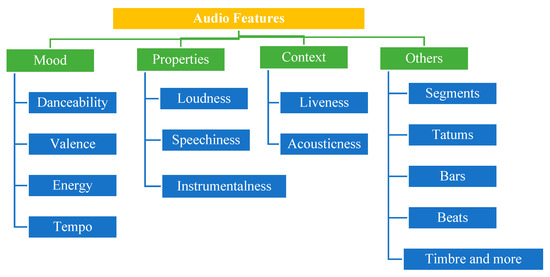
Figure 1.
Audio features.
Danceability defines how suitable a piece is for dancing based on a combination of certain musical elements. A value of 0.0 means it is the least danceable and 1.0 is the most danceable. Acousticness is a measure from 0.0 to 1.0 of whether the track is acoustic and energy is a measure between 0.0 and 1.0. Typically, energetic pieces feel fast, loud, and boisterous.
Instrumentalness predicts whether a track contains no vocals. The closer the instrumentalness value is to 1.0, the greater likelihood the track contains no vocal content. Liveness and loudness are the music features in which the former detects the presence of an audience in the recording, higher liveness represent an increased probability that the track is performed alive, and the later defines the overall loudness of a track is in decibels (dB). Loudness values are averaged across the entire track. Typical range of values change from −60 db to 0 db.
Speechiness detects the presence of spoken words in a track. The more exclusively speech-like the recording e.g., talk show, reading of audio book and poetry, the closer to 1.0 the attribute value. Similarly, tempo defines the overall estimated tempo of a track is determined in beats per minute (BPM). In musical terminology, tempo is the speed or pace of a given piece and derives directly from the average beat duration. Lastly the valence is a measure from 0.0 to 1.0 describing the musical positiveness conveyed by a track. Tracks with high valence sound more positive e.g., happy, cheerful, euphoric, while tracks with low valence sound more negative e.g., sad, depressed, angry.
Machine learning and artificial intelligence are directly related with each other and it explained the ability of a machine to produce intelligent human behavior. Artificial intelligence performs complicated operations for solving human problems. Machine learning inserts a large amount of data through computer algorithm to analyze and provide decision and recommendation of the input data [6,7,8,9].
Several popular music listening platforms, particularly the Spotify platform, have billions of intercepted songs. These songs, as well as underplayed songs, are available in songs not loved by listeners. One of the reasons these unpopular songs are unpopular is that people do not enjoy them. In addition, the song’s technical and audio features are important. In order for the song to be listened to a lot, these features need to be improved and significant audio elements that influence the number of listings need to be identified.
In the current dataset, there are musical terms and information about popular songs. By looking at the correlation values, the variables affecting the popularity of the music were determined. Three different machine learning models have been established, where these variables are the input and the popularity is the target variable. Other variables that have little or no relation to the popularity of music were also used as inputs in these three different machine learning algorithms. These algorithms with different inputs were compared according to the accuracy values of the training and test data.
In this work, the most significant sound characteristics of a song in the music market were determined using the method of filter feature selection and logistic regression, random forest, and K-nearest neighbor (KNN). Our main contributions are summarized below:
- (1)
- This article shows how effective the feature selection method is in determining the properties that are most effective on the popularity of songs.
- (2)
- This article provides a comprehensive study and evaluation comparing the performance of machine learning algorithms in the method of feature selection. Performance criteria have been used to determine the best algorithm.
The purpose of this article is to determine the factors that affect the popularity of a song, to determine whether these determined factors are sufficient for popularity alone, and how effective the other variables in the used dataset are on popularity, using machine learning algorithms. With this study, it can be determined which sound elements should be given more importance by the artists while creating a work. In this way, the popularity of a new song can be determined before it is released.
The paper is structured as follows. A review of relevant studies is described in Section 2. Section 3 contain the information about the dataset. Section 4 contains the evaluation of the accuracy of the established models along with material and method. Section 5 the results obtained along with comparison of benchmark schemes. Finally, Section 6 contains the conclusions and recommendations.
2. Literature Survey
It noticed that various studies examined the Spotify data in the literature. In [10], the behavior of Spotify active users is examined. The paper investigated the system dynamics such as the tracks played, session lengths, and the downtime. In [11], the effect of the promotion process of the music pieces on the number of playlists is investigated. Goldmann and Kreitz have examined the general network features and performance through the number of IP addresses by collecting the network information of the Spotify application via NAT devices [12]. In [13], the marketing strategy of the Spotify application has been emphasized. Likewise, the financial impacts created on music market and its effective growth adventure by its advertising policies have been researched. Kurt et al. conducted a personalized music study by the Spotify application in the paper. They have recommended an appeal to user pleasure through real-time resting molds [14]. In [15], a Spotify application uses digital ads in which the content for the users is investigated. [16] searched the physiology and historical background of the sound, and then created content. In a study by An et al., they used music lyrics to analyze and classify Chinese music according to emotion and the creation of four different datasets. They used the Naive Bayes algorithm, which is one of the most effective algorithms for text classification. Apart from the Naive Bayes algorithm, four different classification algorithms were trained with different datasets and their performances were reported. The performances of the trained algorithms were evaluated and the final accuracy was determined as 68% [17].
Guimaraes et al. used different machine learning algorithms to classify the words in the lyrics of Brazilian music. According to the frequency of the words in the lyrics, they guessed which Brazilian music type the song belonged to [18]. In a study by Duru and Yüreğir, a statistical analysis of the database consisting of 43,936 pieces in the Turkish Music repertoire was made. Determinations were made about the rhythm, which is the basis of music, the “usûl” used in Turkish Music, and the prosody element and its importance in the lyrics that are thought to be directly related to it. The importance of data cleaning was mentioned in the process. As a result of the analysis of the data, it has been revealed that the use of the aruz meter is more in the works composed before the 20th century [19]. In a study by Karatana and Yıldız, the music genres of the songs were determined by using machine learning methods. Certain features were obtained by passing the songs through the signal processing stage, and a classification study was carried out using machine learning algorithms with these features [20].
Sciandraa and Spera show the relationship between song data audio features obtained from the Spotify database (e.g., key and tempo) and song popularity, measured by the number of streams that a song has on Spotify. In the study, special attention was paid to the popularity of the songs, under the research question “What are the determinants of popularity?”, the features that are considered important in making a song popular were determined, while doing this, Beta Regression, generalized linear mixed models (GLLM), beta GLLM were used. In the study, the songs of the artist named Luciano Ligabue were used as a sample application. As a result of the application, it was determined that while Speech, Instrumentality, and Vitality were the features that negatively affected the Popularity Index, the Energy, Value, and Duration of the song were the features that had a positive effect [21].
Trpkovska et al. focused on analyzing the audio characteristics of tracks on Spotify’s Top Songs of 2017 list. In the analysis, information is provided about the common features of popular songs and why people prefer these songs. In the study, estimating one sound feature based on others, searching for patterns in the sound properties of songs, and which properties are related to each other were performed using data visualization and data mining [22].
In the study by Pareek et al., the popularity of the song was estimated using Random Forest classifier, K-Nearest neighbor classifier and Linear Support Vector classifier algorithms and song metrics available in Spotify. Which of these algorithms predicted popularity effectively was determined by looking at the accuracy, precision, recall, and F1-score metrics. When the results were examined, it was observed that the random forest algorithm gave the best result in estimating popularity [23].
Mora and Tierney compared and evaluated Feature Engineering, Feature Selection, and Hyperparameter Optimization algorithms using the Spotify Song Popularity dataset in their study. As a result of this study, Feature Engineering has a greater effect on model efficiency compared to alternative approaches [24].
Zangerle et al. presented an approach that predicts hit songs using low- and high-level sound features in their work. They used deep neural network architecture while performing the prediction process. While predicting the hit song, the input set has been enriched by adding the release year information to the low and high sound features. The findings show that the proposed approach is better than the approaches that use only low- and high-level audio features [25].
In the Nijkamp research, ‘Is Spotify’s audio-based attribution approach effective in explaining streaming popularity on Spotify?’ aimed to answer the research question. The question was analyzed using Spotify’s audio capabilities, taking an attribute-based approach to a success prediction model for the number of streams a song has on Spotify. The results of the correlations showed that there were significant relationships and the aspects of the relationships were in line with the hypotheses, and these relationships were calculated to be weak. It has been determined that the determined sound characteristics alone are insufficient to predict the count of streams [26].
The most similar method to the one that we aimed is the method developed by Rahardwika et al. Rahardwika et al. have investigated the effect of feature selection on the accuracy of music genre classification by using the SVM classifier. In their study, they used Spotify music data. In the feature selection stage, they combined some features in different combination groups (FC1, FC2, FC3, FC4). They proved that each combination group has different accuracy results in the classification results. They suggested the combination of FC1 and FC2 features because the combination of features FC1 and FC2 gives the same accuracy of 80%, but because FC2 has fewer features, logically shorter computation time, because it contains fewer features. Features were included in the FC2 acousticness, instrumentalness, popularity, energy, danceability, speechiness, valence, loudness, tempo, and artist_name. In our method, we have studied the accuracy of feature selection with machine learning algorithms to the classification of music popularity. We have used the filter feature selection method when determining effective features over popularity. The success of algorithms created with both datasets was evaluated by using the F-score value [27]. The properties that influence popularity, through the methods that we use, are instrumentality, acousticness, mode, valence, danceability, energy, loudness. Like our work, this study found that the most effective features in classification of the music genre are acousticness, instrumentality, popularity, energy, danceability, speechiness, valence, loudness, tempo, and artist_name. The fact that a song is popular is an important case in the music field. Moreover, above all other studies, we try to help people in this area by selecting the most beneficial and most important characteristics for popularity.
In this section, a comparison of the machine learning models established using the features selected according to the correlation values and the machine learning models established without feature selection is made. The aim is to learn how these variables, which do not affect popularity, affect the performance of machine learning models. In addition, in this section, a comparison of the studies using methods such as the ones we used is made. The comparison of the studies performed is shown in Table 1.

Table 1.
Comparison of protocols.
3. Dataset
Spotify Music Dataset downloaded from the page www.kaggle.com (accessed on 29 August 2022) contains with a total of 130.663 music with 17 features in the form of acquired metadata. It shows the technical features and popularity rankings of some music tracks that have attracted high interest until today. The appearance of some data from the imported datasets is shown in Table 2.
Table 2.
Some of the imported data.
It shows the technical features and popularity rankings of some music tracks that have attracted high interest until today. The acousticness variable in Table 2 refers to the acoustic value, the danceability variable refers to the beat strength and rhythm, the energy variable to the loudness and its harmony with the rhythm, the liveness variable to the rhythmic balance, the loudness variable to the noise and the tempo variable refers to the BPM.
4. Methodology
This section provides a concise and precise description of the experimental results, their interpretation, as well as the experimental conclusions that can be drawn. In this study, several classifications were using Spotify API via Kaggle software [28]. While the independent variables in the dataset (API) represents musical attributes, the dependent variables represent popularity. There are 130663 observation units in the Spotify API used in this study. The independent variables in this dataset are continuous numerical variables. The dependent variables are an ordinal scale that is an ordered categorical variable. During performing the research, various technological tools have been used in this study. In this study, the datasets are analysis through this platform. In addition, during the analysis process, this platform was used for some subjects in terms of research and learning.
As shown in Figure 2, first, the data are collected, and then a dataset is created. In the step of receiving the data, the data are pulled from the dataset. During the data preparation phase, the data are processed through some processes. In this study, first, data preprocessing steps were made, and then feature selection was performed by removing unimportant variables from the dataset. Models are created using data and different machine learning algorithms. Analyzes are performed with the established models. The previous steps are repeated until the algorithms give the best result. The obtained results are evaluated and the best model is selected.
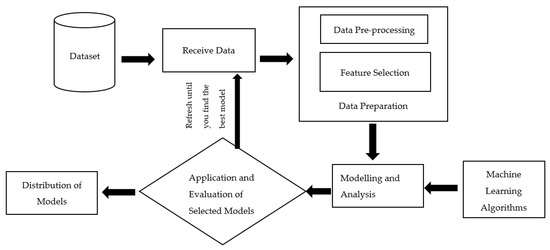
Figure 2.
Workflow diagram of the study.
Jupyter Notebook is an open-source program that provides an interactive environment for programming languages, where both explanation and code can work interactively on the same screen. It was chosen for analysis in this study as an interactive report.
Pandas’ library was used to support for using and manipulating multidimensional data. Scikit used machine learning because it is a library that supports for structuring data, modeling, and explaining variable relations through the model.
In this study, the dataset is analyzed by integrating the dataset into the Jupyter Notebook code editor. Variables are changed where they are required to alter in dataset properties such as types of variables. The unwanted data were removed from the dataset and then the missing data are analyzed. The necessary methods are applied, the outlier data are analyzed mathematically and its results are obtained visually. Corrections are made in the dataset based upon the results. The dataset can be analyzed and it becomes interpretable. Discovery data analysis and data visualizations provide us an opinion regarding structuring of the dataset. In the discoverer data analysis section, summary statistics of the dataset are generated. The classes and class frequencies of the variables and their internal distribution structures are also observed by visualization and tabular methods. Statistical analysis is performed on the pre-processed data and meaningful information is produced from the data by using machine learning algorithms.
4.1. Data Pre-Processing
One of the operations to be performed based on the dataset is to make the data responsive to the operation to be performed. This process is called data preprocessing. Data preprocessing steps are carried out just before starting the work by determining a model on the data. Data pre-processing steps are provided in Figure 3.
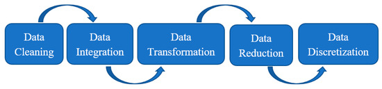
Figure 3.
Data pre-processing steps.
As shown in Figure 3, data cleaning is the process of inserting missing data and fixing, repairing, or removing incorrect or unrelated data from a dataset. Data integration is the merging of data from different sources and the introduction of transformed data to users. Data transformation (normalization) means lowering the input value. When data differ too much, it takes data into a single pattern. The goal is to make it comparable by moving data from a different system to a common system. Data reduction includes volume reduction, data compression, removal of trivial attributes. Data discretization refers to a method that makes it easier to evaluate and manage data by converting a large number of data values into smaller values.
Detecting and Extracting Outliers from the Dataset
The first step we perform on the dataset is to deduct the outliers from the dataset. The outlier finding operation on the datasets was performed with the following pseudo codes.
- Outlier Data Query and Deletion Algorithm
- Q1 = np.percentile(data[c],25)
- Q3 = np.percentile(data[c],75)
- IQR = Q3–Q1
- Outlier_step = 1.5 × IQR
- outlier_list_col = data[(data[c] < Q1 − outlier_step)|(data[c] > Q3 + outlier_step)].index
An outlier is any data point that differs substantially from the rest of the observations in a dataset. In other words, it is an observation that goes beyond the general trend. The algorithm given below was used to find these values. In the first and second lines of the algorithm, the first and third quarter calculations are made. After this calculation, the interquartile range (IQR) is calculated. The quartiles gap is the name given to the difference between the 75% and 25% values of the datasets. In other words, the quartiles represent the middle 50% of the data. This shows us how the mean values are spread out. As a general expression, values that are 1.5 times less than the 25% quartile and 1.5 times more than the 75% quartile are classified as outliers. The outlier’s data in the sample variable are given as shown in Figure 4.
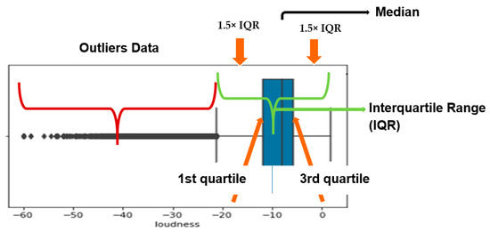
Figure 4.
Loudness feature outlier data.
A total of 798 outliers were detected when this transaction was applied to the dataset. These values have been removed from the dataset.
4.2. Categorizing the Popularity Variable
The most important variable in our data is the popularity variable. Popularity shows the song’s ranking on the most listened playlists. We organized the popularity variable in the dataset as popular and unpopular. In the process, we have given value 1 to popular songs and value 0 to unpopular songs. It has been looked at the average of data in the popularity column at to determine what popular songs were. The average of variables in the popularity column were found as to be 24. According to this average value, songs that are 24 and below are labeled as popular i.e., 1, and songs above it is labeled as unpopular (i.e., 0). After the data were re-edited, it has been determined that 71,709 popular songs and 58156 unpopular songs are found in the dataset.
4.3. Feature Selection
Feature selection is an important method in data mining and machine learning that reduces data size. Feature selection is to create a new feature subset from all the features in the dataset [29,30]. Some of the most important reasons for using the feature selection may include ensuring faster training of the machine learning algorithm, reducing the complexity of a model and facilitating interpretation, and reducing overfitting. There are three main ways to feature selection:
- Filter methods
- Wrapper method (Forward, Backward)
- Embedded methods (Lasso-L1, Ridge-L2 Regression)
In this study, we have used the filter methods. The filter method sorts each property relative to some single-variable metrics, and then selects the highest-order properties amongst them. The wrapper method requires to use a method which is for searching for the blanks of all possible subsets of properties, learning and evaluating a classifier with a subset of these properties. It is considered that the embedded methods be both as a mixture of filter and spiral (wrapper) methods in variable selection, and farther it is as a different approach style. In the feature selection phase, first, the correlations between the independent variables and the target variable are checked. The variables with positive and negative high correlations are shown in Figure 5.
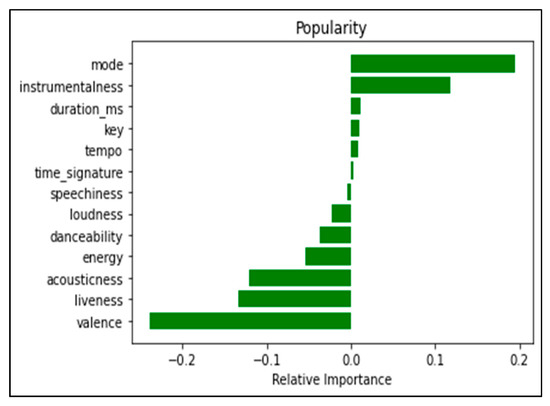
Figure 5.
Variables with positive and negative correlation.
The graph shown in Figure 5 is the correlation of each property with our target variable. It is required that the properties which are highly associated with the target variable are kept. This means that the input property has a high impact on predicting the target variable. We have set the threshold at 0.02 when selecting important features with the filter method. When determining input variables, we selected variables in which their correlation with the target variable is higher than 0.02. This threshold value is determined by the success results of models set up with other threshold values. Best bet is taken at this threshold (e.g., threshold = 0.1, random forest = 57.83%, logistics regression = 58.53%, kNN = 55.42%). In this case, the variables to be used as input in popularity classification are instrumentalness, acousticness, liability, mode, valence, danceability, energy, loudness as shown in Figure 6. The datasets set up without selecting feature selection is given as shown in Figure 7.
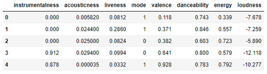
Figure 6.
Features selected by feature selection.
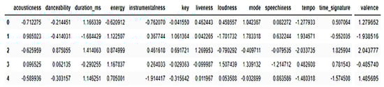
Figure 7.
Features used without feature selection.
5. Results and Discussion
The dataset used in this research is the Spotify music dataset which contains a music dataset with 17 features and 130,663 music. To process this data, Python programming language has been used.
5.1. Separate Dataset
The selected music data are the input data and the target column is the popularity of the music. Moreover, the music data are divided into 66% training data and 33% test data in each experiment. The number of popular and unpopular songs on the dataset is unstable. This affects the success rate of the machine learning algorithms used. The make_classification function is used to prevent this imbalance. The make_classification function is also used to synchronize the distribution of classes in unbalanced datasets as shown in Figure 8.
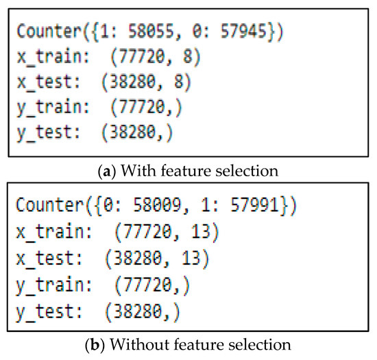
Figure 8.
Dataset balanced using Make_Classification function.
5.2. Classification Using Logistic Regression-Random Forest-KNN Algorithms and Evaluation
Statistical analysis is performed on the pre-processed data and meaningful information is produced from the data by using machine learning algorithms. Algorithms used in modeling: logistic regression, KNN, decision trees (random forest).
Logistic regression is one of the basic classification methods used in estimating categorical variables. The purpose of logistic regression is to find the most appropriate model to describe the relationship between a set of independent (predictive or explanatory) variables related to the bidirectional properties (dependent variable = response or outcome variable). Logistic regression models have been widely used in the fields of biology, medicine, economy, agriculture, veterinary medicine, and transportation in recent years [31].
Random forest is one of the most popular supervised learning methods in machine learning. The RF algorithm is an algorithm consisting of a combination of decision trees, and the trees with the highest accuracy and independence are preferred among the decision trees used [25,32]. It is a tree type classification algorithm that produces multiple classifiers and classifies new data according to the prediction results of these classifiers [33]. Each of the trees is branched according to the features in the datasets. Branching depends on decision points in these features [34].
KNN algorithm is one of the most common algorithms. While classifying, the distance of each record in the database from other records is calculated. Distance measures such as Euclidean and Manhattan are used to measure the distance between data [35]. With the number of neighbors parameter, it is determined with how many neighbors the comparison will be made with the nearest neighbors to the data [36]. In KNN, the goal is to find the nearest predetermined number of training examples closest to the new point and guess the label from them [37].
The F1-score value is used to evaluate the success of machine learning algorithms. The F1 score is the weighted average of precision and recall. F1 is more widely used than accuracy. The main reason that the F1 score value is used instead of accuracy is to not make a faulty model selection in unevenly distributed datasets. F1 Score is very important to us, as it requires a measurement metric that includes not only False Negative or False Positive but also all error costs. We have calculated the precision, recall, and F1-Score rates as follows as shown in Equations (1)–(3).
TP represents the number of real positives, FP—the number of false positives, and FN represents the number of wrong negatives. Whereas precision is defined as the number of true positives and the number of correct positives over the number of false positives, Callback is defined as the number of real positives and the number of real positives over the number of false negatives. The F1-score values of the algorithms used in the study are given in Table 3.
Table 3.
F1-score values in the popularity classification of algorithms.
The F1-score results presented in Table 3 show that the feature selection has a significant impact on accuracy. Confusion matrix was used to see how many of the classes were correctly and how many incorrectly predicted in the popularity classification by the algorithms. Confusion matrix, machine learning, and statistical classification are presented in a tabular layout to visualize the performance of a classifier in problems [38,39]. In a confusion matrix, the columns correspond to the actual genre, the rows to the predicted genre as shown in Figure 9 [40,41].
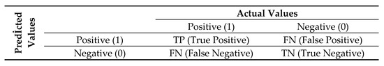
Figure 9.
Confusion matrix.
When the confusion matrix of the random forest algorithm, which was created by feature selection, was examined, it correctly predicted 18,093 of the 19,245 popular songs in the test data. Algorithm correctly guessed 18,329 out of 19,035 unpopular songs. When the confusion matrix of the random forest algorithm, which was created without feature selection, was examined, it correctly predicted 17,933 out of 19,101 popular songs in the test data. Algorithm correctly guessed 18,493 out of 19,179 unpopular songs as shown in Figure 10.
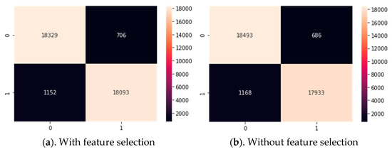
Figure 10.
Confusion matrix of random forest algorithm.
When the confusion matrix of the logistic regression algorithm, which was created by feature selection, was examined, it correctly predicted 17621 of the 19245 popular songs in the test data. Algorithm correctly guessed 18190 out of 19035 unpopular songs. When the confusion matrix of the logistic regression algorithm, which was created without feature selection, was examined, it correctly predicted 17439 out of 19101 popular songs in the test data. Algorithm correctly guessed 18319 out of 19179 unpopular songs as shown in Figure 11.
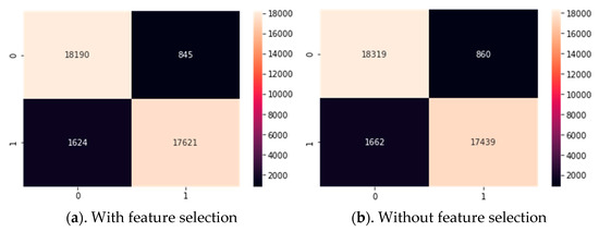
Figure 11.
Confusion matrix of logistic regression algorithm.
When the confusion matrix of the KNN algorithm, which was created by feature selection, was examined, it correctly predicted 17625 of the 19245 popular songs in the test data. Algorithm correctly guessed 18186 out of 19035 unpopular songs. When the confusion matrix of the KNN algorithm, which was created without feature selection, was examined, it correctly predicted 17010 out of 19101 popular songs in the test data. Algorithm correctly guessed 18073 out of 19179 unpopular songs as shown in Figure 12.
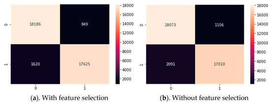
Figure 12.
Confusion matrix of KNN algorithm.
6. Conclusions and Recommendations
This study sheds light on people who work in the related field about the effect of music parameters on popularity. In the study, first, the datasets were made suitable for analysis with data preprocessing. By using filter feature selection, variables (features) associated with popularity were determined and feature selection was applied. Outliers in the variables to be used in the popularity classification were determined and removed from the datasets. In the popularity variable, data ranking 24 and less than 24 are labeled as 1, and values below it are labeled 0.
The work uses the filter feature selection method. The reason why the wrapper and embedded feature selection methods are not used is that models built using these methods produce lower results. For example, in models built with the selection of wrapper feature selection method, the random forest algorithm had 57.73% success, logistics regression algorithm had 58.59%, kNN algorithm had 55.48% success.
While the datasets are separated as training and test data, the make_classification function is used to distribute the classes evenly. 66% of the dataset was used as training data and 33% as test data. The difference in the number of samples of the classes in the training and test data of the models built without feature selection is due to the excess of input features.
When the F1-score ratios of the established algorithms in the test data are examined, the accuracy rates of the test data in the algorithms created by the feature selection process are higher than the models established without feature selection. In this case, it is possible to classify popularity with only popularity-related features, without features with low correlation values. Among all the algorithms used, the algorithm with the highest accuracy is the random forest algorithm. Both models with and without feature selection are more successful than other algorithms. The success rate of the model with feature selection in the random forest algorithm is higher.
Future research may look at these models to create different prediction models to predict the song’s popularity. They can expand this study by using data from different platforms (Tik Tok, YouTube Shorts) instead of song popularity. In future studies, words that affect popularity can be determined by examining the words of popular music. This type of work can be of great help to music artists and producers.
Author Contributions
This manuscript was designed and written by F.K. and I.T., B.C.K. conceived the main idea of this study. H.S.A. and M.F. wrote the program and conducted all experiments. A.B.A. and Y.-I.C. supervised the study and contributed to the analysis and discussion of the algorithms and experimental results. All authors have read and agreed to the published version of the manuscript.
Funding
This research was supported by Korea Agency for Technology and Standards in 2022, project numbers are, K_G012002234001 and the MSIT(Ministry of Science and ICT), Korea, under the ITRC(Information Technology Research Center) support program(IITP-2022-2017-0-01630) supervised by the IITP(Institute for Information & communications Technology Promotion) and Gachon University research fund of 2019(2019-0784).
Conflicts of Interest
The authors declare no conflict of interest.
References
- Li, T.; Ogihara, M.; Tzanetakis, G. Music Data Mining; CRC Press: Boca Raton, FL, USA, 2012; Available online: https://www.routledge.com/Music-Data-Mining/Li-Ogihara-Tzanetakis/p/book/9781439835524 (accessed on 15 July 2022).
- Sloboda, J.A.; O’Neill, S.A.; Ivaldi, A. Functions of music in everyday life: An exploratory study using the Experience Sampling Method. Music. Sci. 2001, 5, 9–32. [Google Scholar] [CrossRef]
- Prabhu, N.R.; Vasko, J.A.; Bein, D.; Bein, W. Music genre classification using data mining and machine learning. Inf. Technol. -New Gener. 2018, 738, 397–403. [Google Scholar]
- Popular Music. Available online: https://tr.wikipedia.org/wiki/Pop%C3%BCler_m%C3%BCzik (accessed on 29 June 2022).
- Spotify. Audio Features & Analysis. 2021. Available online: https://developer.spotify.com/discover/ (accessed on 10 October 2022).
- Khan, M.A.; Abbas, S.; Raza, A.; Khan, F.; Whangbo, T. Emotion Based Signal Enhancement Through Multisensory Integration Using Machine Learning. CMC-Comput. Mater. Contin. 2022, 71, 5911–5931. [Google Scholar] [CrossRef]
- Ayvaz, U.; Gürüler, H.; Khan, F.; Ahmed, N.; Whangbo, T. Automatic Speaker Recognition Using Mel-Frequency Cepstral Coefficients Through Machine Learning. CMC-Comput. Mater. Contin. 2022, 71, 5511–5521. [Google Scholar] [CrossRef]
- Iqbal, M.W.; Naqvi, M.R.; Khan, M.A.; Khan, F.; Whangbo, T. Mobile Devices Interface Adaptivity Using Ontologies. CMC-Comput. Mater. Contin. 2022, 71, 4767–4784. [Google Scholar] [CrossRef]
- Laila, U.E.; Mahboob, K.; Khan, A.W.; Khan, F.; Taekeun, W. An Ensemble Approach to Predict Early-Stage Diabetes Risk Using Machine Learning: An Empirical Study. Sensors 2022, 22, 5247. [Google Scholar] [CrossRef] [PubMed]
- Zhang, B.; Kreitz, G.; Isaksson, M.; Ubillos, J.; Urdaneta, G.; Pouwelse, J.A.; Epema, D. Understanding User Behavior in Spotify. In Proceedings of the 2013 Proceedings IEEE INFOCOM, Turin, Italy, 14–19 April 2013; pp. 220–224. [Google Scholar]
- Aguiar, L.; Waldfogel, J. Platforms, Promotion and Product Discovery: Evidence from Spotify Playlist; National Bureau of Economic Research: Cambridge, MA, USA, 2018; pp. 1–44. [Google Scholar]
- Goldmann, M.; Kreitz, G. Measurements on the Spotify Peer-Assisted Music on Demand Streaming System. In Proceedings of the IEEE International Conference on Peer-to-Peer Computing, Kyoto, Japan, 31 August–September 2011. [Google Scholar]
- Vonderau, P. The Spotify Effect: Digital Distribution and Financial Growth. SAGE J. 2017, 20, 3–19. [Google Scholar] [CrossRef]
- Jacobson, K.; Murali, V.; Newett, E.; Whitman, B.; Yon, R. Music personalization at Spotify. In Proceedings of the 10th ACM Conference on Recommender Systems, Boston, MA, USA, 15–19 September 2016; p. 373. [Google Scholar]
- Efe, A. Example Of Online Music Platform as A Display Advertising Space: Spotify. Int. J. Public Relat. Advert. Stud. 2019, 2, 131–146. [Google Scholar]
- Canyakan, S. Audio History: Audio-Specific Music Technology and Origin. Uşak Univ. J. Soc. Sci. 2017, 10, 171–191. [Google Scholar]
- An, Y.; Sun, S.; Wang, S. Naive Bayes classifiers for music emotion classification based on lyrics. In Proceedings of the 2017 IEEE/ACIS 16th International Conference on Computer and Information Science, Wuhan, China, 24–26 May 2017; pp. 635–638. [Google Scholar]
- Guimaraes, P.; Froes, J.; Costa, D.; Freitas, L.A. A comparison of identification methods of Brazilian music styles by lyrics. In Proceedings of the Fourth Widening Natural Language Processing Workshop, Online, 4 December 2020; pp. 61–63. [Google Scholar]
- Duru, S.; Yüreğir, O.H. Data Cleaning for Data Mining and Applications on Turkish Classical Music Data. J. Econ. Adm. Sci. 2019, 3, 150–159. [Google Scholar]
- Karatana, A.; Yıldız, O. Music Genre Classification with Machine Learning Techniques. In Proceedings of the 25th Signal Processing and Communications Applications Conference, Antalya, Turkey, 15–18 May 2017; pp. 1–4. [Google Scholar]
- Sciandra, M.; Spera, I.C. A model-based approach to Spotify data analysis: A Beta GLMM. J. Appl. Stat. 2022, 49, 214–229. [Google Scholar] [CrossRef] [PubMed]
- Apostolova-Trpkovska, M.; Kajtazi, A.; Abazi Bexheti, L.; Kadriu, A. Applying Data Mining and Data Visualization within the Scope of Audio Data Using Spotify; IADIS: Lisbon, Portugal, 2019; pp. 197–204. [Google Scholar] [CrossRef]
- Pareek, P.; Shankar, P.; Sakariya, N. Predicting Music Popularity Using Machine Learning Algorithm and Music Metrics Available in Spotify. J. Dev. Econ. Manag. Res. Stud. JDMS 2022, 9, 10–19. [Google Scholar]
- Cueva Mora, A.; Tierney, B. Feature Engineering vs. Feature Selection vs. Hyperparameter Optimization in the Spotify Song Popularity Dataset. In Proceedings of the Tenth International Conference on Data Analytics, Barcelona, Spain, 3–7 October 2021. [Google Scholar]
- Zangerle, E.; Vötter, M.; Huber, R.; Yang, Y.H. Hit Song Prediction: Leveraging Low-and High-Level Audio Features. In Proceedings of the 20th International Society for Music Information Retrieval Conference, Delft, The Netherlands, 4–8 November 2019; pp. 319–326. [Google Scholar]
- Nijkamp, R. Prediction of Product Success: Explaining Song Popularity by Audio Features from Spotify Data. Bachelor’s Thesis, University of Twente, Enschede, The Netherlands, 2018. [Google Scholar]
- Rahardwika, D.S.; Rachmawanto, E.H.; Sari, C.A.; Susanto, A.; Mulyono IU, W.; Astuti, E.Z.; Fahmi, A. Effect of feature selection on the accuracy of music genre classification using SVM classifier. In Proceedings of the 2020 International Seminar on Application for Technology of Information and Communication (iSemantic), Semarang, Indonesia, 19–20 September 2020; pp. 7–11. [Google Scholar]
- Available online: https://www.kaggle.com/tomigelo/spotify-audio-features (accessed on 15 July 2022).
- Pan, J.S.; Tian, A.Q.; Chu, S.C.; Li, J.B. Improved binary pigeon-inspired optimization and its application for feature selection. Appl. Intell. 2021, 51, 8661–8679. [Google Scholar] [CrossRef]
- Hu, P.; Pan, J.S.; Chu, S.C. Improved binary grey wolf optimizer and its application for feature selection. Knowl.-Based Syst. 2020, 195, 105746. [Google Scholar] [CrossRef]
- Bircan, H. Logistic Regression Analysis: An Application on Medical Data. Kocaeli Univ. J. Soc. Sci. 2004, 8, 185–208. [Google Scholar]
- Özdemir, S. Potential Distribution Modelling and Mapping Using Random Forest Method: An Example of Yukarigökdere District. Turk. J. For. 2018, 19, 51–56. [Google Scholar] [CrossRef]
- Aksoy, G.; Ataş, P.; Karabatak, M. Investigation of shopping habits using data mining classification algorithms. In Proceedings of the 2019 1st International Informatics and Software Engineering Conference (UBMYK), Ankara, Turkey, 6–7 November 2019; pp. 1–5. [Google Scholar]
- Breiman, L. Random forest. Mach. Learn. 2001, 45, 5–32. [Google Scholar] [CrossRef]
- Cover, T.; Hart, P. Nearest Neighbor Pattern Classification. Information Theory. IEEE Trans. 1967, 13, 21–27. [Google Scholar]
- Jiang, Y.; Zhou, Z.H. Editing Training Data For Knn Classifiers with Neural Network Ensemble. Lect. Notes Comput. Sci. 2004, 3173, 356–361. [Google Scholar] [CrossRef]
- Veranyurt, Ü.; Deveci, A.; Esen, M.F.; Veranyurt, O. Disease Classification by Machine Learning Techniques: Random Forest, K-Nearest Neighbor and Adaboost Algorithms Applications. Int. J. Health Manag. Strateg. Res. 2020, 6, 275–286. Available online: https://dergipark.org.tr/en/pub/usaysad/issue/56571/786740 (accessed on 15 July 2022).
- Han, J.; Pei, J.; Kamber, M. Data Mining: Concepts and Techniques; Elsevier: Amsterdam, The Netherlands, 2011. [Google Scholar]
- Japkowicz, N. Performance Evaluation for Learning Algorithms; Cambridge University Press: Cambridge, UK, 2011. [Google Scholar]
- Alan, A.; Karabatak, M. Evaluation of the Factors Affecting Performance on the Datasets—Classification Relationship. Fırat Univ. J. Eng. Sci. 2020, 32, 531–540. [Google Scholar]
- Tzanetakis, G.; Cook, P. Musical genre classification of audio signals. IEEE Trans. Speech Audio Process. 2002, 10, 293–302. [Google Scholar] [CrossRef]


Publisher’s Note: MDPI stays neutral with regard to jurisdictional claims in published maps and institutional affiliations. |
© 2022 by the authors. Licensee MDPI, Basel, Switzerland. This article is an open access article distributed under the terms and conditions of the Creative Commons Attribution (CC BY) license (https://creativecommons.org/licenses/by/4.0/).