Attributation Analysis of Reinforcement Learning-Based Highway Driver

Abstract

While machine learning models are powering more and more everyday devices, there is a growing need for explaining them. This especially applies to the use of deep reinforcement learning in solutions that require security, such as vehicle motion planning. In this paper, we propose a method for understanding what the RL agent’s decision is based on. The method relies on conducting a statistical analysis on a massive set of state-decisions samples. It indicates which input features have an impact on the agent’s decision and the relationships between the decisions, the significance of the input features, and their values. The method allows us to determine whether the process of making a decision by the agent is coherent with human intuition and what contradicts it. We applied the proposed method to the RL motion planning agent which is supposed to drive a vehicle safely and efficiently on a highway. We find out that making such an analysis allows for a better understanding of the agent’s decisions, inspecting its behavior, debugging the ANN model, and verifying the correctness of the input values, which increases its credibility.

1. Introduction

1.1. Motivation

Machine learning is increasingly applied in everyday devices and computer applications. Beyond making popular applications more attractive with AI, researchers are trying to use it to solve real-world complex problems [1]. One such challenge is to plan the motion of the automated vehicle on the highway in a safe and effective manner. A promising approach to this problem is the application of deep reinforcement learning (RL) [2] methods which use artificial neural networks (ANN) to train the decision-making agents. However, the use of ANN-based methods introduces the black-box factor, which makes agents’ decisions unpredictable and therefore increases operational risk. Such a factor is ineligible in the applications whose safety must be verified and proved. Therefore, the utilization of ANN-based methods to plan the vehicle motion on the road, without understanding the ANN decisions, may be risky for the system’s end-user.

Knowing this threat, we propose the evaluation method of RL agents based on interpretable machine learning (IML) techniques combined with a statistical analysis. The presented solution is intended to decipher the black-box model by analyzing the neural activations in the distribution of possible inputs with respect to agent decisions. Our method allows an investigation of whether the agent’s decisions are consistent with the assumptions and the ANN decision process matches human intuition. Additionally, it enables debugging the model itself and detecting the data or model corruption. The proposed method is created for inspecting RL-driven applications whose decisions are critical for safety and the confirmation of proper functioning is required.

1.2. Contribution

In this work, we present a novel method of evaluation of two DRL agents which are designated to plan the behavior to achieve a safe and effective highway driving experience. The first agent (Maneuver agent) selects the appropriate discrete maneuvers (follow lane, prepare for lane change (left/right), lane change (left/right), and abort) and the second one (ACC agent) controls the continuous value of the acceleration. On the basis of these two trained agents, we propose an evaluation method based on an Integrated Gradient [3] and a further statistical analysis. The analysis consists of an ANOVA, a t-test, and an examination of a linear (Pearson [4]) and monotonic (Spearman Rho [5]) correlation. We describe our experiments and show the results of the analyses of agents operating in a discrete and continuous action space. Additionally, we specify the applicability and relevance of such methods.

2. Related Work

2.1. RL in AV

Over the past few years, there has been an increasing interest in the use of RL in the motion planning of automated vehicles. In the literature, we can find multiple examples of the applications of RL for typical driving scenarios, such as lane keeping, lane changing, ramp merging, overtaking, and more. For example, [6] proposed to train a driving policy with the DQN algorithm [7] to decide whether it is worthwhile to change lanes to the left or right or to keep the lane. The training took place in a simulated three-lane highway environment. The agent’s objective was to drive safely and smoothly and maintain efficiency. A similar solution was proposed in [8] where the authors considered a comparable environment and action space. Additionally, the work emphasized the safety assurance, integrating the RL methodology with the Responsibility-Sensitive Safety framework [9], which guarantees at least to not cause a collision.

A more challenging environment was solved in [10], where the authors focused on training agents to handle unsignalized intersections. To successfully navigate through the junction, the agent had to learn other drivers’ intentions and predict their movement. It is supposed to drive to the destination as fast as possible and avoid a collision. The agent obtained a positive reward for achieving the target lane, a large negative reward for a collision, and a small punishment for each step of the simulation.

Another work [11] introduced a novel solution based on reinforcement learning combined together with a classical A* algorithm. The authors presented a model-based RL algorithm that depends on a tree search where the heuristic is learned with the DQN algorithm. Such an approach allows for the increased control and understanding of the algorithm. A more detailed overview of the works on the application of RL in motion planning can be found in [12,13].

2.2. Explainable RL

As the application of machine learning becomes more popular, the demand for its interpretability has increased. This is due to the need to increase the credibility and fairness of models [14] and raise the level of people’s trust. Initially, a field of interpretable machine learning (IML) has been developed, partially focused on the interpretation of neural networks activation. The interpretation relies on calculating how the output of the ANN was impacted by each element of the given part of the network. For example, by the input features, as in the case of Primary Attributation [3,15,16,17]. In the case of Layer Attributation [18,19,20], it regards the impact of each neural layer and each single neuron activation in the case of Neuron Attributation [15,18].

However, the eXplainability of RL (XRL) goes beyond understanding a single neural activation. That is because of the temporal dependency between consecutive states and the agent’s actions that induce the next visited states. A sequence of transitions may be used to interpret the agent’s action concerning the long-term goal. Additionally, it is also important that the objective of agent training is maximizing the sum of the collected rewards rather than mapping the inputs to the ground-truth label as in the case of supervised learning. These additional features allow for explaining the behavior of RL agents in an introspective, causal, and contrasting way.

The recent advances in XRL were categorized in [21] into two major groups: transparent algorithms and post hoc explainability. The group of transparent algorithms includes those whose models are built to support their interpretability. Such an approach is implemented in hierarchical RL [22,23] where the major task is decomposed for sub-tasks with a trained higher-level agent and lower-level agents. The hierarchical structure is designed to provide an understanding of the agent’s decision-making processes. Another approach is simultaneous learning which learns both the policy and explanation at the same time. An example work [24] which proposed to learn multiple Q-functions, one for each meaningful part of the reward, to understand predictions about future rewards. The last type of transparent learning is representation learning which involves learning latent features to facilitate the extraction of meaningful information by the agent models. The representative work [25] proposes to reconstruct the observation with autoencoders, a training model to predict the next state, or a train inverse model to predict the action from the previous state.

However, DRL algorithms are not natively transparent; therefore, post hoc explainability is more common and debated in this paper. It relies on an analysis of the states and neural activations of transitions executed with an already-trained agent.

One of the post hoc methods is saliency maps [20,26] which may be applied to convolutional neural networks (CNN) with images as input. This method generates a heatmap that highlights the most relevant information for a CNN on the image. A similar approach was used in [27] to measure the relevance of network layers and units to decrease the ANN size by removing their less relevant part. Another interesting work is [28] which proposed a three-step analysis of agent transitions in order to classify interesting agent interactions and present them in a visual form. However, from our perspective, understanding individual decisions is not enough to interpret the general behavior of an agent.

3. Preliminaries

3.1. Reinforcement Learning Agents

Our experiment intends to develop a method of interpreting RL agent decisions, adequate for discrete and continuous action space. For this purpose, we train two separate agents. The first one (Maneuver agent) is responsible for planning appropriate maneuvers to be executed. Agent’s action space is discrete and contains six items: follow lane, prepare for lane change (right, left), lane change (right, left), and abort maneuver. The objective of the agent is to navigate in the most efficient way while preserving the gentleness desired on the roads. Expected behaviors are, for example, changing to the faster lane if the ego’s velocity is lower than the speed limit or returning to the right lane when it is possible and worthwhile.

The second agent (ACC agent) is responsible for planning the continuous value of acceleration when Follow Lane maneuver is selected by the higher-level agent. Reward function is incentive for the agent to drive as fast as possible in terms of the speed limit, keep a safe distance to the vehicle ahead, increase comfort by minimizing jerks, and avoid collisions.

The training uses a simulation [29] of a highway environment in which parameters, such as the number of lanes, traffic flow intensity, characteristics of other drivers’ behavior, and vehicle model dynamics, are randomized, providing diverse traffic scenarios.

3.2. Integrated Gradients

Integrated Gradients (IGs) [3] are an example of the Primary Attributation method which aims at explaining the relationship between models’ output with respect to the input features by calculating the importance of each feature for the model’s prediction. For calculation, an IG needs baseline input $x^{\prime }$ which is composed arbitrarily and should be neutral for the model. For example, if the model consumes images, the typical baseline is an image that contains all black or white pixels. IG, firstly, in small steps, $\alpha$ generates a set of inputs by linear interpolation between the baseline and the processed input x. Then, it computes gradients between interpolated inputs and model outputs (Equation (1)) to approximate the integral with the Riemann Trapezoid rule.

$$\begin{array}{cc}\hfill & IntegratedGradient{s}_i\left(x\right)::=(x_i-x_i^{\prime })\times {\int }_{\alpha =0}^1{\displaystyle \frac{\delta F(x^{\prime }+\alpha \times (x-x^{\prime }))}{\delta x_i}}d\alpha \hfill \\ \hfill & \mathrm{where}i=\mathrm{feature};x=\mathrm{input};x^{\prime }=\mathrm{baseline};\alpha =\mathrm{interpolation}\mathrm{constant}\hfill \end{array}$$

(1)

4. Description of Experiment

4.1. Neural Networks

We train the Maneuver and ACC agents (Section 3.1) with PPO algorithm [30]. Agents are based on similar neural network architecture (Figure 1) which differs only on the last control module part and slightly on the first layers due to different definitions of input. The ANN is fed with an observation of the current traffic situation in the form of feature vectors. The first vector describes the state of the ego vehicle (descriptive statistics for those parameters are stored in Table 1) and consists of its longitudinal velocity ($ego\_ve{l}_s$), level of speed limit execution ($ve{l}_{s\_limit\_exec}=setspeed/ve{l}_s$), longitudinal acceleration ($ac{c}_s$), and last selected action (ACC agent $ac{c}_{s\_last}$; Maneuver agent $las{t}_{m}aneuver$). Observation for Maneuver agent also consists of lateral position $po{s}_{f}cs.d$, velocity $ve{l}_d$ and acceleration $ac{c}_d$, rotation toward center of the lane $ro{t}_{f}cs$, and information whether is safe to change lane for both sides.

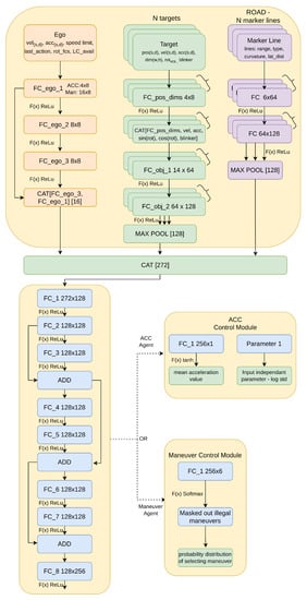
Figure 1. ANN architecture takes as an input vector the representation of traffic situation. It processes input through feed-forward layers and 3 residual blocks. Each agent has a different control module that produces the probability distribution parameters of selecting an action and slightly different input layers due to the different definitions of observations. FC—fully connected layers with bias; CAT—operation of features concatenation; means that layers have shared weights (e.g., each target is processed by the same layer).

Table 1. Table includes main descriptive statistics for training parameters regarding ego vehicle. Observed real values were normalized within predefined ranges during the creation of input feature vector to the neural network.

Training Parameter	Mean	St. Dev	Min	Median	Max
ego_f_pos_fcs.d	−1.03	0.10	−2.06	−1.03	0.04
real_ego_f_pos_fcs.d	−0.054	0.20	−2.12	−0.06	2.09
ego_f_vel_s	0.52	0.13	0.06	0.50	0.77
real_ego_f_vel_s	25.92	6.29	2.85	25.11	38.63
ego_f_vel_s_limit_execution	0.97	0.07	0.17	1.00	1.48
ego_f_vel_d	0.00	0.09	−1.00	−0.00	1.00
real_ego_f_vel_d	0.00	0.36	−4.00	−0.00	4.00
ego_f_acc_s	0.00	0.04	−0.60	0.00	0.45
real_ego_f_acc_s	0.01	0.38	−6.00	0.00	4.50
ego_f_acc_d	0.00	0.01	−0.19	0.00	0.25
real_ego_f_acc_d	0.00	0.01	−0.38	0.00	0.50
ego_f_rot_fcs	−0.00	0.00	−0.05	−0.00	0.05

The second feature vector represents perceived vehicle on the road and includes relative to the ego information about longitudinal and lateral distance ($(po{s}_s,po{s}_d)$), velocity ($ve{l}_s,ve{l}_d$), and acceleration ($ac{c}_s,ac{c}_d$). It also consists of data about target’s rotation ($ro{t}_{v}cs$) and its dimensions ($(ob{j}_{width},ob{j}_{length})$). The last vector represents the road by encoding each visible marker line with information about delimiter type, curvature, and rotation in the ego’s position, sensing range, and lateral distance from the ego to the line.

Input is passed through the feed-forward layers as presented in Figure 1. Encoded features in the latent state are processed by 3 residual blocks [31] which outputs go to control module. In the case of the ACC agent, ANN produces the parameters of the gaussian distribution—mean, and log std. The mean value is produced by the $tanh$ activation function, and log std is the input-independent trainable parameter. In the case of the Maneuver agent, the control module passes the output from residual blocks with softmax activation and masks those maneuvers which are not available from the safety perspective according to rules defined in [9] implemented in [8].

4.2. Reward Functions

The reward functions vary for both agents because their objectives are different. The ACC agent reward $R_{acc}$ is a weighted sum of the following terms:

• Speed limit execution $Speed\_ex$—calculated as a ratio of ego velocity and speed limit; forces agent to maximize speed limit.
• Squared acceleration $Ac{c}^2$—the squared value of acceleration; negative reward promotes smooth ride.
• Jerk absolute $Jer{k}_{abs}$—the value of absolute jerk; also promotes comfort driving experience.
• Safety violation $Sv$—a negative reward for being too close to other vehicles. Distance is calculated based on Responsibility-Sensitive Safety assumptions [9].
• Terminal state $TS$—a reward for causing a collision or speeding too much.

$$R_{acc}=0.07\ast Sp\_ex-0.02\ast Ac{c}^2-0.0001\ast Jer{k}_{abs}-0.2\ast Sv-10\ast TS$$

(2)

Reward function for training Acc agent. All terms are defined to return positive values so the weight sign indicates whether it is positive reinforcement (+) or negative (−).

The Maneuver agent reward $R_{maneuver}$ terms are as follows:

• Speed limit execution cube $Speed\_e{x}^3$ calculated as a ratio of ego velocity and speed limit—forces agent to maximize speed limit, encourages to overtake slower cars.
• Negative acceleration Squared $Neg\_ac{c}^2$—a reward for braking events, incentives for smooth driving.
• Sequence maneuver execution $Seq\_Man\_exec$—a reward for inconsistency in selecting maneuvers, this term has non-zero value when agent selects different action then selected before. It reduces action flickering problem.
• Collision $Col$—a negative reward for causing collision.
• Right lane available $Right\_L\_avail$—non-zero when the right lane is available and the agent can change to it. It promotes gentleness on road by releasing the left lane for faster vehicles.
• Being overtaken by right $B\_OverTake\_R$—this reward is non-zero when the agent is slower than vehicles in the right lane. The agent should change the lane to the right to allow faster vehicles to drive on the left.
• Overtaking right $Over\_Take$—this term rewards agents for overtaking other cars while driving on the left lane.

$$\begin{array}{cc}\hfill & R_{maneuver}=0.03\ast Speed\_e{x}^3-0.0005\ast Neg\_ac{c}^2-0.0001\ast Seq\_Man\_exec\hfill \\ \hfill & -1\ast Col-0.03\ast Right\_L\_avail-0.01\ast B\_OverTake\_R+0.07\ast Over\_Take\hfill \end{array}$$

(3)

Reward function for training Maneuver agent. All terms are defined to return positive values; therefore, the weight sign indicates whether it is positive reinforcement (+) or negative (−).

All terms of reward functions are defined to return positive values; therefore, the weight sign indicates whether it is positive reinforcement (+) or negative (−).

4.3. Agent Training

Both trainings last more than 30 M steps Figure 2. Agents started from random actions, because the neural networks were randomly initialized, and gradually improved their performance. All training hyperparameters are presented in Table 2. Afterward, we select the checkpoints with the highest mean sum of rewards, checking on basic predefined test scenarios whether the agents behave as we expected.

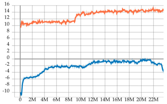
Figure 2. The graph shows the accumulated average sum of rewards (Maneuver agent-orange and ACC agent-blue) during the episodes between optimization steps. The training typically achieves its best performance at some point and then, after more iterations, either keeps the performance or degrades it. Then, to obtain the best agent, we choose the checkpoint with the highest mean sum of rewards (22 M step for the Maneuver agent and 20 M step for the ACC agent). The difference between the reward levels is due to the different definitions of the reward function.

Table 2. Table includes major hyperparameters of PPO algorithm used for training ACC and Maneuver agents. The trainings were performed with the usage of RLlib [32].

Training Parameter	Maneuver	ACC
gamma	0.9985	0.998
lambda	0.95	0.95
batch size	1024	50,000
mini batch size	512	20,000
steps	38 M	30 M
best checkpoint step	22 M	20 M
grad_clip	3.0	3.0
lr	4.5 × 10−5	0.0001
num_gpu	1	1
sgd_iter	3	3
workers	80	80

An example of a test scenario for the ACC agent consists of a single-lane road with an ego and front target which accelerates and decelerates interchangeably. The expected ego behavior is to follow the target, minimizing acceleration oscillation. From the beginning of training, agent often loses track of the target or speeds up and crashes into it. Over the training iteration, agent learns how to track the target and tries to keep minimum acceleration to drive smoothly.

An example of a testing scenario for Maneuver agent consists of ego and a slow target car in front of ego, driving on the right lane on three-lane road. Agent’s task is to overtake a vehicle and return to the right lane. In the beginning, the agent only follows the target, then changes the lane to the most left because it learns that this is the fastest lane. Toward the end of the training, the agent learns to return to the right lane after overtaking because of the 3 terms of the reward function: $Right\_L\_avail,B\_OverTake\_R,Over\_Take$—(Equation (3)).

4.4. Collecting Neural Activations

Having selected the checkpoints, we run an evaluation of agents in randomly generated scenarios generating 5 h driving experience for the Maneuver agent and 3.5 h for the ACC agent. This corresponds to over 240,000 simulation steps. From this set, every tenth sample was selected to ensure their temporal independence for statistical analysis. The samples consist of state inputs and agent decisions—action value for ACC agent and probabilities of selecting particular action in case of Maneuver agent. Based on that data, we calculate the attributation of each input value using the Integrated Gradients method, Section 3.2. As a baseline input, we select a feature vector that represents three-lane highway with no other vehicles besides the ego in its default state (max legal velocity, 0 acceleration). For calculation, we use Captum library [33] (BSD licensed) which provides an implementation of a number of IML methods, Section 2.2, for PyTorch models. The results of attributations calculation with associated input features and ANN’s decisions are further inspected with statistical analysis.

4.5. Statistical Analysis

The statistical analysis consists of two parts. For all calculations, we use the Minitab software [34]. The first part focuses on the examination of the level of significance of the attributation values and the analysis of their distribution. The second one studies the relationships between attributation values, values of input features, and probabilities of selecting maneuvers in the case of the Maneuver agent.

4.5.1. ANOVA and t-Tests

The first step of statistical analysis of attributation is to identify parameters with statistically significant parameters of attributation distribution regarding the selected item from action space for the Maneuver agent and overall distribution for the ACC agent. The next step is to perform an analysis of variance for the set of parameters determined in the first step. To do so, we divide attributation data according to the type of maneuver into six groups. Attributations that regard objects and roads are summed up according to each one of the characteristic parameters for those aspects. Then, we perform t-test for every parameter with Null hypothesis $H_0:\mu =0.03$ and alternative hypothesis $H_1:\mu >0.03$. We assume the significance level of all tests as $\alpha =0.05$. Based on those results, we decide which distributions of parameters have a significantly higher mean value than 0.03, distinguishing between different maneuvers. Finally, we perform Welch’s ANOVA [35] for results that are significantly based on the t-test which gives us information about which parameters were significantly more important than others regarding available maneuver. Samples were divided into groups with additional post hoc test (Games Howell [36]). To visualize distinguished results, we calculate the standard deviation for those samples and $95\%$ confidence intervals for their means, which gives us $95\%$ assurance that the expected value is within those intervals regarding the dispersion of data.

4.5.2. Correlation Tests

The second part of the analysis relies on the examination of the linear and monotonic relationship between feature attributation and the probability of selecting a given maneuver. We apply a Pearson correlation [4] to study linear correlation and Spearman’s rank correlation coefficient Rho [5] to examine a monotonic correlation. Correlations are calculated for the attributation of all input features concerning the probability of selecting a particular maneuver. Additionally, for the ACC agent, we calculated mutual information for action and features/attributation (Table 3).

Table 3. Table with values of highest mutual information for action of ACC agent with respect to values of ego’s features and attributation.

Mutual Information
Feature	MI
ego_acc_s	1.658
ego_last_action_acc	1.074
attr_obs_acc_s	0.621
attr_ego_last_action_acc	0.350
attr_ego_vel_s	0.273
road_att_lat_dist	0.272
attr_ego_vel_s_limit_exec	0.248
road_att_closes_in	0.244
obj_att_pos_s	0.196
obj_att_pos_d	0.159

An analysis based on a Pearson correlation begins with the calculation of the p-value and identification of whether the correlation is significant at 0.05 $\alpha$-level. The p-value indicates whether the correlation coefficient is significantly different from 0. If the coefficient effectively equals 0, it indicates that there is no linear relationship in the population of compared samples. Afterward, we interpret the Pearson correlation coefficient itself to determine the strength and direction of the correlation. The correlation coefficient value ranges from $-1$ to $+1$. The larger the absolute value of the coefficient, the stronger the linear relationship between the samples. We take the convention that the absolute value of a correlation coefficient lower than 0.4 is a weak correlation, the absolute value of a correlation coefficient between 0.4 and 0.8 is a moderate linear correlation, and if the absolute value of the Pearson coefficient is higher than 0.8, the strength of the correlation is large. The sign of the coefficient indicates the direction of the dependency. If the coefficient is positive, variables increase or decrease together and the line that represents the correlation slopes upward. A negative coefficient means that one variable tends to increase while the other decreases and the correlation line slopes downward.

The fact that an insignificant or low Pearson correlation coefficient exists does not mean that no relationship exists between the variables because the variables may have a nonlinear relationship. Considering that, we utilize Spearman’s rank correlation coefficient Rho [5] to examine the monotonic relationship between samples. In a monotonic relationship, the variables tend to move in the same relative direction but not necessarily at a constant rate. To calculate the Spearman correlation, we have to rank the raw data and then calculate its correlation. Test also consists of the significance test; the Spearman Rho correlation coefficient describes the direction and strength of the monotonic relationship. The value is interpreted analogously as the Pearson values. To visualize results and look for other types of relationships, we created scatterplots for different pairs of samples.

5. Results

We inspect the results of the statistical analysis in the following way. Firstly, we examine the boxplots which visualize the distribution of attributation for a particular maneuver for each input signal. From the plots, we can easily see how much a given feature contributes to choosing a given maneuver. For example, Figure 3 presents the distribution of attributation of the feature ego_pos_fcs.d which indicates the ego’s lateral distance from the driving lane center. We can see that the middle 50% of the distributions (box), mean (dot), and median (horizontal line in the box) of the attributation values lie much higher for the maneuvers connected to a lane change. For the follow lane and abort maneuvers, an attributation higher than 0 is considered an outlier (star). This behavior is in line with the driver’s intuition and proves to us that the neural network works as intended, at least in this individual field.

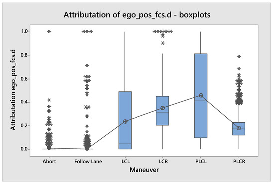
Figure 3. Distributions of attributation values for one of the ego parameters (distance from the center of lane) for all maneuver types.

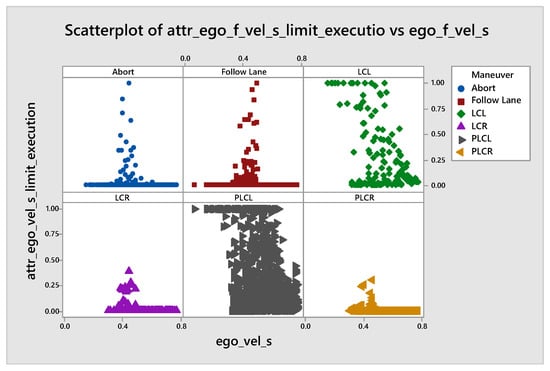
Next, we examine the correlation between attributations and the values of the input features. We check this in two directions. Firstly, we look at the strong correlations and compare them with human intuition. For example, in Table 4 and Table 5, we notice that the agent, while considering selecting the Follow Lane maneuver, pays less attention to the value of the longitudinal velocity (vel_s) while the velocity grows, and the same applies to acceleration. On the other side, it is more attentive to the parameter which informs about fulfilling the velocity limit (vel_s_limit) while the velocity grows. This attitude is shown by the Spearman Rho correlation; however, the Pearson does not reveal it. This behavior can be explained by the fact that during a Follow Lane maneuver, we usually care less about the absolute velocity of other vehicles because we do not want to overtake them. Instead, we focus on achieving the speed limit, speed increases, and if we are close to that goal, we focus on not exceeding the speed limit. Additionally, we confirm that by inspecting the scatterplots of the vel_s and vel_s_limit attributations presented in Figure 4. One of our other results showed behavior that contradicts human intuition. During the overtaking maneuver (lane change), we expect that the position of other objects is important while the ego velocity grows, but our results show a negative correlation.

Table 4. Table with values of Pearson correlation for attributation of vel_s_limitation with respect to values of ego’s features. Red highlights a strong correlation, and yellow—medium strength of correlation.

PEARSON
ego	Follow Lane	PLCL	PLCR	LCL	LCR	Abort
pos_fcs.d	0.064	−0.026	−0.186	−0.157	−0.122	−0.21
vel_s	−0.05	0.063	−0.116	−0.124	−0.408	−0.305
vel_s_limi	0.204	−0.895	0.182	0.166	−0.916	0.786
vel_d	−0.014	0.056	0.07	0.17	−0.042	−0.137
acc_s	−0.024	−0.025	−0.082	−0.054	−0.062	−0.39
acc_d	0.008	0.173	−0.031	0.023	0.011	−0.254
rot_fcs	−0.017	0.06	0.093	−0.121	−0.146	−0.105

Table 5. Table with values of Spearman Rho correlation for attributation of vel_s_limitation with respect to values of features which describe ego state. Red color means strong correlation, and yellow—medium strength of correlation.

Spearman Rho
ego	Follow Lane	PLCL	PLCR	B	LCR	Abort
pos_fcs.d	0.135	0.121	−0.078	0.108	−0.165	0.039
vel_s	−0.688	−0.657	0.557	−0.472	−0.061	−0.28
vel_s_limi	0.877	0.858	−0.938	0.646	−0.978	0.52
vel_d	0.016	0.035	0.011	0.006	−0.156	0.095
acc_s	−0.636	−0.642	0.49	−0.493	−0.267	−0.099
acc_d	0.02	0.023	−0.009	0.014	0.068	−0.143
rot_fcs	0.031	0.054	−0.001	0.017	−0.171	0.094

Figure 4. Scatterplot shows a comparison between ego’s longitudinal velocity (vel_s) and attributation values of vel_s_limit (velocity normalized to speed limit) for all maneuvers. Values of correlations for those examples can be found in Table 4 and Table 5.

We believe that such behavior is similar to human drivers, because they, while speeding up, stop thinking about absolute speed and start being concerned with if they drive with a legal velocity, comparing their velocity with the speed limit.

As regards the ACC agent, we identify a medium-strength correlation between the attributation of acceleration and the value of the acceleration action. It means that the agent pays more attention to the value of acceleration when it increases. This is a desired correlation, but in our opinion, the values of attributation should be higher. The expected attributation values and correlations are based on a review prepared by a team of five experts working on the use of AI/ML in autonomous vehicles. In the future, this type of analysis should be conducted based on extensive research on human eye movements in various driving scenarios. In Figure 5, we notice that there exist at least three different patterns of correlations. They are connected to factors not analyzed in this experiment, and it is probably beneficial to investigate further. To do so would require the preparation of a non-random set of evaluation scenarios based on which it would be possible to differentiate reasons for various patterns in attributation correlations. It is also worth noticing that passed parameters for other road users are summarized and coded in a non-intuitive manner for humans. This would require an additional analysis in order to separate the influence of objects of the same type in terms of their relation to the ego vehicle (i.e., the front target).

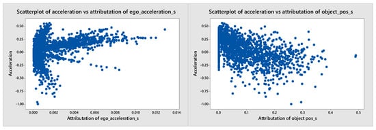
Figure 5. Scatterplot present the correlation between acceleration of continuous agent and attributation of its acceleration value and position of other objects.

Another interesting correlation we found is the fact that the agent seems to focus slightly more on the other vehicles’ positions when it is braking (see Figure 5). This is also a desired and justified effect because the braking intensity should depend on the intensity of the changes in the object’s position in relation to the ego. When there is no need to brake, it is more important to know the speed of the objects, which determines the stability of the situation.

Secondly, we deliberate where the strong correlation should occur to match human intelligence. For example, we assume that the driver should compare the longitudinal distance to the target vehicle with its velocity. Therefore, the correlation between the attributation of the objects’ position with respect to the longitudinal velocity should be strong. The analysis indicates only a weak strength of the correlation, thus contrary to the assumptions.

Additionally, the results inspection allows us to detect two types of errors in our model. While looking at the scatterplots (e.g., Figure 4, which demonstrates the value of the attributation with respect to the input feature values, we easily detected that one’s feature (lateral position) is normalized to the range (−2, 0) instead of (−1, 1). This allows us to fix the implementation of the agent’s observations.

The second finding regards the ANN architecture. Because this method is not intended to discover the vanishing gradient problems, the lack of attributation for every sample in one region of the input features made us aware of this problem in our model. The wrong implementation of the tensors’ concatenation does not pass the gradients through the model and deprives the agent of using part of the input knowledge. The correction of that error eliminates the vanishing gradients problem and increases the agents’ performance.

6. Application

The presented method may contribute to a better understanding of the behavior of reinforcement learning agents whose consecutive decisions came from sampling from the distribution generated by the ANN. First of all, it allows for identifying which input features influence the agent’s decisions the most and inspecting the correlation between the importance of a given input feature to its value. It enables checking whether the ANN decision process matches human intuition (e.g., the faster the agent drives, the more it pays attention to the value of acceleration). Besides that, such an analysis enables detecting errors present in the model itself (e.g., vanishing gradients—important information is ignored) or in input data (e.g., the charts shows the wrong data distribution caused by the incorrect implementation of the normalization function). Thanks to that, we had an opportunity to fix these two issues by improving the model architecture and by fixing the implementation of the data normalization. In our opinion, the application of the presented method increases the safety and predictability of the entire system. In the case of AV motion planning, it may lead to an increase in the reliability of RL applications, in the opinion of OEMs and consumers. Furthermore, the results of the presented method may be utilized for the improvement of the ANN architecture or to enhance the training process. The enhancement of the learning process may start by tuning the reward function to better represent the driver’s objective. For example, if the results point out that the agent does not pay attention to the other objects, then we propose to add to the reward some term that depends on the objects (e.g., the reward is based on the time to collision metric). On the other hand, the ANN architecture may be further enhanced by redesigning the modules that process features that are neglected. By appealing to the issue of disregarding objects, we may propose to redesign that part, for example, by using proven architecture, such as that presented in [37].

7. Discussion

Knowing what the agent is paying attention to can be calming for the end user and build confidence in the model. This, in addition to the evaluation performed with Key Performance Indicators (KPIs), may increase the model’s reliability. However, knowing on what basis an agent makes decisions does not explain why the agent makes them. It still does not solve the problem of the RL explainability. We may only assume that an examination of the behavior in a significant number of situations expounds us the agent’s character.

One more thing to discuss is a situation when an agent’s evaluation metrics (KPIs) are high, but the analysis results contradict it. This may indicate that either the KPI definitions are wrong, or the model uncovers correlations in feature inputs that are not obvious to humans but still correct. Nevertheless, such a situation may decrease the reliability of ANN-based models and discourage their application.

8. Conclusions

In this paper, we present the method for the detailed inspection of the ANN model of the RL agent. The statistical methods applied to collect samples of agent decisions allow for the recognition of agents’ behavior patterns by looking globally at the overall behavior and not at an individual action. This is achieved by the analysis of attributation distribution, differentiated by the considered maneuver and juxtaposed with values of other parameters describing the situation. By inspecting the analysis results, we can seek confirmation that an ANN concentrates on input features which are also important for a human driver. With the examination of the correlation between the attributation and feature values, we find a pattern that matches human intuition and that which is contrary to it. This knowledge helps us improve the model by changing the model architecture, enhancing the training process, and ensuring that decisions are made in accordance with an environment evaluation that prioritizes safety and effectiveness.

References

- MacKay, D.J.C. Information Theory, Inference, and Learning Algorithms; Cambridge University Press: Cambridge, UK, 2003. [Google Scholar]
- Sutton, R.S.; Barto, A.G. Reinforcement Learning: An Introduction; A Bradford Book: Cambridge, MA, USA, 2018. [Google Scholar]
- Sundararajan, M.; Taly, A.; Yan, Q. Axiomatic Attribution for Deep Networks. In Proceedings of the 34th International Conference on Machine Learning, ICML 2017, Sydney, Australia, 6–11 August 2017; Volume 7, pp. 5109–5118. [Google Scholar]
- Freedman, D.; Pisani, R.; Purves, R. Statistics (International Student Edition), 4th ed.; Pisani, R.P., Ed.; WW Norton & Company: New York, NY, USA, 2007. [Google Scholar]
- Zar, J.H. Spearman rank correlation. In Encyclopedia of Biostatistics; John Wiley & Sons, Ltd.: Hoboken, NJ, USA, 2005. [Google Scholar]
- Wang, P.; Chan, C.; de La Fortelle, A. A Reinforcement Learning Based Approach for Automated Lane Change Maneuvers. arXiv 2018, arXiv:1804.07871. [Google Scholar]
- Mnih, V.; Kavukcuoglu, K.; Silver, D.; Graves, A.; Antonoglou, I.; Wierstra, D.; Riedmiller, M.A. Playing Atari with Deep Reinforcement Learning. arXiv 2013, arXiv:1312.5602. [Google Scholar]
- Orłowski, M.; Wrona, T.; Pankiewicz, N.; Turlej, W. Safe and Goal-Based Highway Maneuver Planning with Reinforcement Learning. In Proceedings of the Advanced, Contemporary Control, Łódź, Poland, 25 June 2020; Bartoszewicz, A., Kabziński, J., Kacprzyk, J., Eds.; Springer International Publishing: Cham, Switzerland, 2020; pp. 1261–1274. [Google Scholar]
- Shalev-Shwartz, S.; Shammah, S.; Shashua, A. On a Formal Model of Safe and Scalable Self-driving Cars. arXiv 2017, arXiv:1708.06374. [Google Scholar]
- Isele, D.; Cosgun, A.; Subramanian, K.; Fujimura, K. Navigating Intersections with Autonomous Vehicles using Deep Reinforcement Learning. arXiv 2017, arXiv:1705.01196. [Google Scholar]
- Keselman, A.; Ten, S.; Ghazali, A.; Jubeh, M. Reinforcement Learning with A* and a Deep Heuristic. arXiv 2018, arXiv:1811.07745. [Google Scholar]
- Aradi, S. Survey of Deep Reinforcement Learning for Motion Planning of Autonomous Vehicles. arXiv 2020, arXiv:2001.11231. [Google Scholar] [CrossRef]
- Kiran, B.R.; Sobh, I.; Talpaert, V.; Mannion, P.; Sallab, A.A.A.; Yogamani, S.K.; Pérez, P. Deep Reinforcement Learning for Autonomous Driving: A Survey. arXiv 2020, arXiv:2002.00444. [Google Scholar] [CrossRef]
- Angerschmid, A.; Zhou, J.; Theuermann, K.; Chen, F.; Holzinger, A. Fairness and Explanation in AI-Informed Decision Making. Mach. Learn. Knowl. Extr. 2022, 4, 556–579. [Google Scholar] [CrossRef]
- Lundberg, S.M.; Allen, P.G.; Lee, S.I. A Unified Approach to Interpreting Model Predictions. In Proceedings of the 31st International Conference on Neural Information Processing Systems; Curran Associates Inc.: Red Hook, NY, USA, 2017; Volume 30, pp. 4768–4777. [Google Scholar]
- Shrikumar, A.; Greenside, P.; Kundaje, A. Learning Important Features Through Propagating Activation Differences. In Proceedings of the 34th International Conference on Machine Learning, ICML 2017, Sydney, Australia, 6–11 August 2017; Volume 7, pp. 4844–4866. [Google Scholar]
- Simonyan, K.; Vedaldi, A.; Zisserman, A. Deep Inside Convolutional Networks: Visualising Image Classification Models and Saliency Maps. arXiv 2013, arXiv:1312.6034. [Google Scholar]
- Dhamdhere, K.; Yan, Q.; Sundararajan, M. How Important Is a Neuron? In Proceedings of the 7th International Conference on Learning Representations, ICLR 2019, New Orleans, LA, USA, 6–9 May 2019. [Google Scholar]
- Leino, K.; Sen, S.; Datta, A.; Fredrikson, M.; Li, L. Influence-Directed Explanations for Deep Convolutional Networks. In Proceedings of the 2018 IEEE International Test Conference (ITC), Phoenix, AZ, USA, 29 October–1 November 2018. [Google Scholar]
- Selvaraju, R.R.; Cogswell, M.; Das, A.; Vedantam, R.; Parikh, D.; Batra, D. Grad-CAM: Visual Explanations from Deep Networks via Gradient-based Localization. Int. J. Comput. Vis. 2016, 128, 336–359. [Google Scholar] [CrossRef]
- Heuillet, A.; Couthouis, F.; Díaz-Rodríguez, N. Explainability in deep reinforcement learning. Knowl.-Based Syst. 2021, 214, 106685. [Google Scholar] [CrossRef]
- van Seijen, H.; Fatemi, M.; Romoff, J.; Laroche, R.; Barnes, T.; Tsang, J. Hybrid Reward Architecture for Reinforcement Learning. arXiv 2017, arXiv:1706.04208. [Google Scholar]
- Kawano, H. Hierarchical sub-task decomposition for reinforcement learning of multi-robot delivery mission. In Proceedings of the 2013 IEEE International Conference on Robotics and Automation, Karlsruhe, Germany, 6–10 May 2013; pp. 828–835. [Google Scholar] [CrossRef]
- Juozapaitis, Z.; Koul, A.; Fern, A.; Erwig, M.; Doshi-Velez, F. Explainable Reinforcement Learning via Reward Decomposition. In Proceedings of the International Joint Conference on Artificial Intelligence. A Workshop on Explainable Artificial Intelligence, Macao, China, 10–16 August 2019. [Google Scholar]
- Raffin, A.; Hill, A.; Traoré, R.; Lesort, T.; Rodríguez, N.D.; Filliat, D. S-RL Toolbox: Environments, Datasets and Evaluation Metrics for State Representation Learning. arXiv 2018, arXiv:1809.09369. [Google Scholar]
- Mundhenk, T.N.; Chen, B.Y.; Friedland, G. Efficient Saliency Maps for Explainable AI. arXiv 2019, arXiv:1911.11293. [Google Scholar]
- Yeom, S.; Seegerer, P.; Lapuschkin, S.; Wiedemann, S.; Müller, K.; Samek, W. Pruning by Explaining: A Novel Criterion for Deep Neural Network Pruning. arXiv 2019, arXiv:1912.08881. [Google Scholar] [CrossRef]
- Sequeira, P.; Gervasio, M. Interestingness Elements for Explainable Reinforcement Learning: Understanding Agents’ Capabilities and Limitations. Artif. Intell. 2019, 288, 103367. [Google Scholar] [CrossRef]
- Traffic AI—Simteract. 2018. Available online: https://simteract.com/pl/projects/traffic-ai-pl/ (accessed on 12 September 2022).
- Schulman, J.; Wolski, F.; Dhariwal, P.; Radford, A.; Klimov, O. Proximal Policy Optimization Algorithms. arXiv 2017, arXiv:1707.06347. [Google Scholar]
- He, K.; Zhang, X.; Ren, S.; Sun, J. Deep Residual Learning for Image Recognition. In Proceedings of the 2016 IEEE Conference on Computer Vision and Pattern Recognition (CVPR), Las Vegas, NV, USA, 27–30 June 2016; pp. 770–778. [Google Scholar] [CrossRef]
- Liang, E.; Liaw, R.; Nishihara, R.; Moritz, P.; Fox, R.; Goldberg, K.; Gonzalez, J.; Jordan, M.; Stoica, I. RLlib: Abstractions for Distributed Reinforcement Learning. In Proceedings of the Machine Learning Research; Dy, J., Krause, A., Eds.; JMLR: Cambridge, MA, USA, 2018; Volume 80, pp. 3053–3062. [Google Scholar]
- Kokhlikyan, N.; Miglani, V.; Martin, M.; Wang, E.; Alsallakh, B.; Reynolds, J.; Melnikov, A.; Kliushkina, N.; Araya, C.; Yan, S.; et al. Captum: A unified and generic model interpretability library for PyTorch. arXiv 2020, arXiv:2009.07896. [Google Scholar]
- Minitab, LLC—Version 18. Available online: https://www.minitab.com (accessed on 12 September 2022).
- Liu, H. Comparing Welch’s ANOVA, a Kruskal-Wallis Test, and Traditional ANOVA in Case of Heterogeneity of Variance; Virginia Commonwealth University: Richmond, VA, USA, 2015. [Google Scholar]
- Sauder, D.C.; DeMars, C.E. An Updated Recommendation for Multiple Comparisons. Adv. Methods Pract. Psychol. Sci. 2019, 2, 26–44. [Google Scholar] [CrossRef]
- Vinyals, O.; Babuschkin, I.; Czarnecki, W.M.; Mathieu, M.; Dudzik, A.; Chung, J.; Choi, D.H.; Powell, R.; Ewalds, T.; Georgiev, P.; et al. Grandmaster level in StarCraft II using multi-agent reinforcement learning. Nature 2019, 575, 350–354. [Google Scholar] [CrossRef] [PubMed]
Publisher’s Note: MDPI stays neutral with regard to jurisdictional claims in published maps and institutional affiliations. |
© 2022 by the authors. Licensee MDPI, Basel, Switzerland. This article is an open access article distributed under the terms and conditions of the Creative Commons Attribution (CC BY) license (https://creativecommons.org/licenses/by/4.0/).