In this section, the hierarchical clustering-based image retrieval is implemented, and the computation performance of the retrieval algorithm is analyzed. In addition, the position accuracy of the visual localization is evaluated.
5.1. Experimental Results of Database Image-Clustering Algorithm
Two image databases (namely, the KTH image database [
61] and the HIT-TUM image database) were used to evaluate the performance of the proposed algorithm. The images in the HIT-TUM database were acquired from the Harbin Institute of Technology and the Technical University of Munich. Each database contains 400 images captured in 10 different indoor scenes, such as an office, a corridor, a restaurant, and so on. All data processing was run on MATLAB 2018A with an Intel Core i7 CPU and 8GB RAM. Randomly selected example images in the databases are shown in
Figure 8. It is worth noting that images in the databases are successively captured in indoor scenes, so the visual features extracted from the images captured in the same indoor scene have high correlations.
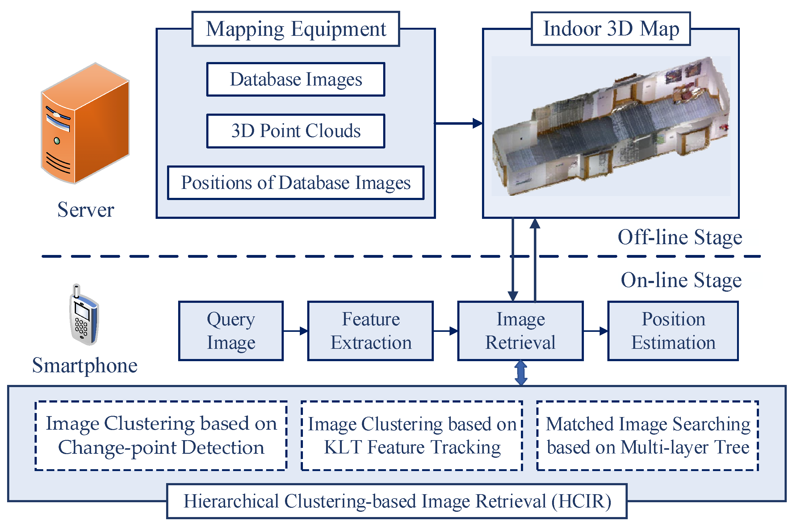
For scene-level image clustering, database images are grouped by their global features based on the CUSUM change-point detection. The results of the scene-level clustering guide the query image to retrieve the clusters that are similar to the query. Therefore, the performance of database image clustering affects the efficiency of the image retrieval system. For an image retrieval system, the efficiency of the retrieval algorithm is reflected in two aspects: the number of searched database images and the time consumption of the image retrieval. Generally, the fewer database images are searched, the less time retrieval takes.
In the same indoor scene, as the database images are successively captured, the Gist features extracted from these images have high correlations. Taking advantage of the correlations, scene-level clustering of database images can be achieved. However, the noise generated in feature extraction affects the correlation of the features. Therefore, the original Gist features of database images need to be pre-processed (including Kalman filtering and Kalman smoothing) to restore the correlation of image features. For a database image, Gist features can be extracted according to different scales and directions. In this paper, Gist features are extracted at three scales and six directions, so 18
feature elements are extracted from each image. That is, the Gist feature vector of each image contains 18 feature elements.
Figure 9 shows an example of the Gist feature pre-processing result of a database image, including the original Gist feature values, Kalman filtering results, and Kalman smoothing results. It can be found from
Figure 9 that the correlation between original feature values is not evident due to the influence of noise. In contrast, by Kalman filtering, noise is effectively suppressed, and the correlations between features are restored. According to Kalman filtering results, more obvious correlations can be obtained by further Kalman smoothing of Gist features. The pre-processing of features recovers the correlations of global features of database images, which is beneficial to scene-level clustering.
Scene-level database image clustering is achieved by detecting the change-points in Gist feature sequences. When image retrieval is executed in the results of scene-level clustering, according to the similarity of the global features, the query image will preferentially search the database image clusters with a higher similarity. Therefore, if all database images in the same scene are grouped into one cluster, the query image captured in this scene can find its matched database images in this cluster. In contrast, if a database image captured in a certain scene is falsely grouped into other clusters, this database image cannot be retrieved when the query searches the right cluster. Depending on the above analysis, the core of the proposed algorithm is that the database images in the same scene are grouped into one cluster as much as possible.
To analyze the performance of the proposed algorithm, scene-level image clustering is executed, and confusion matrices are employed to evaluate clustering accuracy. The confusion matrices of the results of database image clustering are shown in
Figure 10. The confusion matrix used to evaluate clustering accuracy in this paper can also be regarded as a clustering error matrix. The row labels of the matrix are the correct cluster labels, and the column labels are the predicted cluster labels. For the matrix in
Figure 10a, the values in the third, fourth, and fifth rows of the fourth column are 1, 39, and 6, respectively. This set of values shows that for 46 (
) database images that are grouped into one cluster, 39 database images were truly captured in the Office II scene, one image was misclassified into the Corridor II scene category, and six images were misclassified into the Corridor III scene. For a row of the confusion matrix, the sum of all values in that row represents the actual number of images in the cluster. For a column of the confusion matrix, the sum of all values in that column represents the predicted number of images in the cluster. The confusion matrix effectively reflects the performance of the proposed scene-level clustering algorithm. By observing the confusion matrix, it can be known that for image-clustering results, incorrectly grouped images only occur in two adjacent image clusters, and the reason accords with the clustering principle in this paper. Specifically, image clustering acts on the indoor database image sequence, and the change-points are detected based on global features of database images, so that images between two change-points are grouped into one cluster. Therefore, the incorrect image grouping is caused by errors in change-point detection. Obviously, if errors exist in change-point detection, some database images that should belong to a certain cluster are grouped into the former or the latter cluster.
In this paper, four criteria (i.e., recall rate, precision rate, accuracy rate, and F1 score) are used to evaluate the performance of the clustering algorithm. The recall rate
is the ratio of the number of correctly grouped images to the actual number of images in that cluster. The precision rate
refers to the ratio of the number of correctly grouped images to the number of images in the cluster. The accuracy rate
refers to the ratio of the number of correctly grouped images to the total number of images. The F1 score
is used in statistics to measure the accuracy of a classification model. This score can be calculated by the recall rate and the precision rate:
Global features of an image include color features (such as color histogram features and color moment features) and texture features (such as wavelet transform features and Gabor transform features). In simulation experiments, Gist features, color histogram features, color moments, wavelet transform features, and Gabor features are used to perform scene-level clustering on database images, and experimental results are shown in
Table 1. For the experimental results,
,
and
denote the average recall rates, average precision rates, and average F1 scores, respectively. From the results shown in
Table 1, the color features (such as color histograms and color moments) perform weakly on scene-level clustering. The reason is that the color difference of indoor scenes is relatively small. Especially in an environment with a white wall as the main background, it is not easy to distinguish the scenes by the color information. Compared with color features of images, texture features of images perform better in terms of clustering performance, especially for Gabor features and Gist features. Because multiple Gabor filters with different scales and directions are used in extracting Gist features, Gist features describe the textures of scenes more comprehensively, thereby achieving more accurate image-clustering results.
To reveal the clustering performance of the ICSCD algorithm proposed in this paper, two typical change-point detection algorithms (i.e., the mean shift-based algorithm [
36] and the Bayesian estimation-based algorithm [
62]) are simulated for grouping database images at the scene level. The experimental results shown in
Table 2 indicate that the proposed ICSCD algorithm significantly outperforms the Bayesian estimation-based algorithm in four metrics: the average recall rate, the average precision rate, the average F1 score, and the accuracy rate. The reason is that the Bayesian estimation-based algorithm utilizes local features in change-point detection, but the local features are too sensitive to scene changes and tend to group database images belonging to the same scene into multiple image clusters or group images belonging to the same class into other clusters. This also shows that the local features of the images are more suitable for further classification of the scene-level clustering results, which is why local features are used for the second layer of clustering in this paper. Both the proposed ICSCD algorithm and the mean shift-based algorithm use global features for clustering, but the difference is that the change-point detection function
is employed to detect the change points for image clustering in the proposed ICSCD algorithm, whereas the mean shift function is utilized to detect the change points in the mean shift-based algorithm. Since both the influence of the values at the detection position and the influence of the expected values of the parameter models (i.e., the parameter model
A and the parameter model
B in the hypothesis test) within the sliding window (as shown in
Figure 4) are taken account in the change-point detection function
, a higher clustering accuracy can be obtained. Specifically, the average recall rate, the average precision rate, the average F1 score, and the accuracy rate of the proposed ICSCD algorithm are greater than 0.92, which is significantly higher than the mean shift-based algorithm.
5.2. Experimental Results of Hierarchical Image Retrieval and Visual Localization
In the proposed HCIR algorithm, the best-matched database image is determined by the maximum similarity method. Therefore, the validity of the method needs to be verified by experiments. In this part of the experiments, since the best-matched image is the database image that is most similar to the query image, the database image
with the highest matching similarity to the query image is found by the global search, and the index of this database image is
. In addition, another best-matched database image
is determined by the proposed maximum similarity method, and the index of the database image is
. The average error
of the index positions of best-matched database images can be calculated by:
where
is the index error of the best-matched database image in the
i-th experiment, and
is the total number of query images for experiments.
Based on the average error
, the average distance error between the best-matched database images
and
can be further defined by
, where
is the fixed acquisition distance of database images. The average index error
and the average distance error
reflect the performance of retrieving the best-matched database images with the maximum similarity method. For the experimental results, the smaller values of
and
indicate that the matched database images are closer to the query image. The results of matched image retrieval are shown in
Table 3 under the condition that
is set to 10 cm. For the experimental results, the ratio
is the percentage of the number of experimental results that satisfy
. In addition, the average value
of the matching similarity and the average value
of matched feature points are also calculated in experiments.
The experimental results shown in
Table 3 indicate that for image retrieval experiments with the similarity maximum method separately conducted in the KTH database and the TUM-HIT database, the probability of successfully retrieving a matched database image (i.e., the situation of
) exceeds 94%. In other cases, although the similarity between the matched image and the query image cannot reach the maximum value, the index errors are less than 2, which indicates that the matched image is close to the query image, and there are enough matched features between the matching image and the query image. Therefore, the matched database images under the situation of
,
, and
can be used for visual localization. For the two databases, the average error
of the index positions is less than 0.1, and the average distance error is less than 1 cm, showing the effectiveness of the similarity maximum method in determining matched database images. Moreover, the experimental results also show that for different databases, the average matching similarity between the query image and the best-matched database image is greater than 0.5, and there are more than 120 pairs of matched feature points between the query image and the best-matched database image, which provides a fundamental guarantee for visual localization.
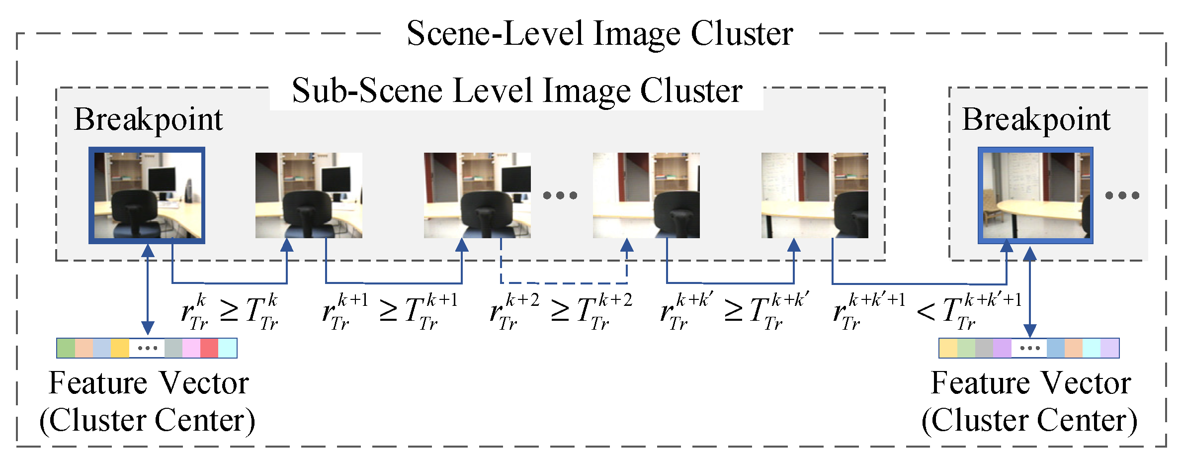
In the proposed HCIR algorithm, the scene-level clustering results are sorted based on the global feature similarity, and then the database images in the sub-scene clusters are sorted based on the local feature similarity. After the two-stage sorting, the query image is matched with database images according to the sorting result. From the above process, it is known that when retrieving the scene-level clustering results based on the global feature similarity, the best case is to obtain the matched image in the first clustering result, and the worst situation is obtaining the matched images after all the results are retrieved. Therefore, for the scene-level image retrieval, the success rate of image retrieval within the top-
K clusters is proposed in this paper to evaluate the performance of the clustering algorithm in image retrieval. Specifically, after scene-level clustering of database images, more than one image cluster can be obtained. If the matched database image can be retrieved after searching
K image clusters, image retrieval is considered to be achieved within
K database image clusters. For a total of
query images, if there are
query images, and their matched database images are in the
K-th cluster, the success rate of the top-
K clusters is defined as
. The success rate effectively reflects the impact of the scene-level clustering algorithm on the performance of image retrieval. The scene-level clustering algorithms of database images can be divided into two categories: one is based on the method of detecting change points of visual features (such as the proposed HCIR algorithm in this paper, the mean shift-based algorithm, and the Bayesian estimation-based algorithm), and another is clustering a fixed number of database images (such as the C-GIST algorithm [
37]). In the C-GIST algorithm, five consecutive database images are grouped into one cluster, and the cluster center is a feature vector of the image that is located at the center position of each cluster. In this paper, two categories of image-clustering algorithms are simulated, respectively, and the success rate of the top-
K clusters is calculated. The results are presented in
Table 4.
The results shown in
Table 4 indicate that the proposed HCIR algorithm is beneficial in improving the success rate of the top-
K clusters for a query image. For the two databases, the success rates of the top-five clusters achieved by the HCIR algorithm, mean shift-based algorithm, and the Bayesian estimation-based algorithm are more than 90%. At the same time, it is not difficult to find that the HCIR algorithm has more obvious performance advantages. Especially in the KTH database, the success rate of the first cluster is 66.75%, and the success rate of the top-five clusters reaches 99.75%. For the HIT-TUM database and the KTH database, the best-matched database image can be retrieved within the top-five clusters by the HCIR algorithm. In addition, for the sub-scene-level image clustering, success rates of the first
K-clusters are also calculated and recorded. Experimental results show that for the HCIR algorithm, the success rate of the first cluster is more than 88%, which indicates that in most cases, the best-matched database image can be found in the first sub-cluster.
To verify the image retrieval efficiency of the proposed HCIR algorithm, image retrieval experiments are performed on the HCIR algorithm and the comparison algorithms. In the experiments, the mean shift-based algorithm, the Bayesian estimation-based algorithm, and the C-GIST algorithm are single-layer clustering algorithms. In addition, another two multi-layer clustering algorithms are considered: the mean shift-KLT algorithm and the Bayesian estimation-KLT algorithm. For the two multi-layer clustering algorithms, database images are firstly grouped by the mean shift-based algorithm or the Bayesian estimation-based algorithm, and then the images are further grouped by the KLT algorithm. According to the average number of retrieved images shown in
Table 5, multi-layer clustering algorithms have higher retrieval efficiency, and the number of similar comparisons (i.e., the processes of feature matching) can be limited to 10% of the database size. The reason is that database images are only grouped into scene-level clusters for the single-layer algorithms, and thus the query image needs to match with database images in the scene-level cluster one-by-one. In contrast, database images are further grouped on the basis of scene-level image clusters in multi-layer algorithms. Then, according to visual similarities, image clusters are ranked, and the query image preferentially matches with the database images in the most similar cluster. Therefore, multi-layer algorithms have a better performance at average numbers of retrieved database images.
It can be observed from the experimental results shown in
Table 5 that fewer database images are retrieved in the HCIR algorithm compared with the other two multi-layer algorithms. The reason is that the ICSCD algorithm has a better performance at scene-level clustering (as shown in
Table 2), so that the cluster center can better express the global features of the images in the cluster.
Table 6 shows the average running time of the image-retrieval system using different clustering algorithms. By comparing the number of retrieved images with the average running time of image retrieval, it can be known that when there are more retrieved database images, the running time consumed by image retrieval is also more. Experimental results shown in
Table 5 and
Table 6 indicate that more database images are retrieved in single-layer clustering algorithms, leading to larger time overheads than in multi-layer clustering algorithms. It is obvious that the HCIR algorithm has advantages in terms of the number of retrieved database images and the running time of image retrieval. The reason is that multi-layer clustering on database images is employed in the HCIR algorithm, and more importantly, the ICSCD algorithm is employed in the proposed retrieval algorithm that achieves a better performance in scene-level database image clustering.
Table 7 shows the average running time of different stages in image retrieval. In the practical implementation of image retrieval, hundreds of local features are needed to be matched between the query image and the database image, resulting in the most time consumption appearing at this stage.
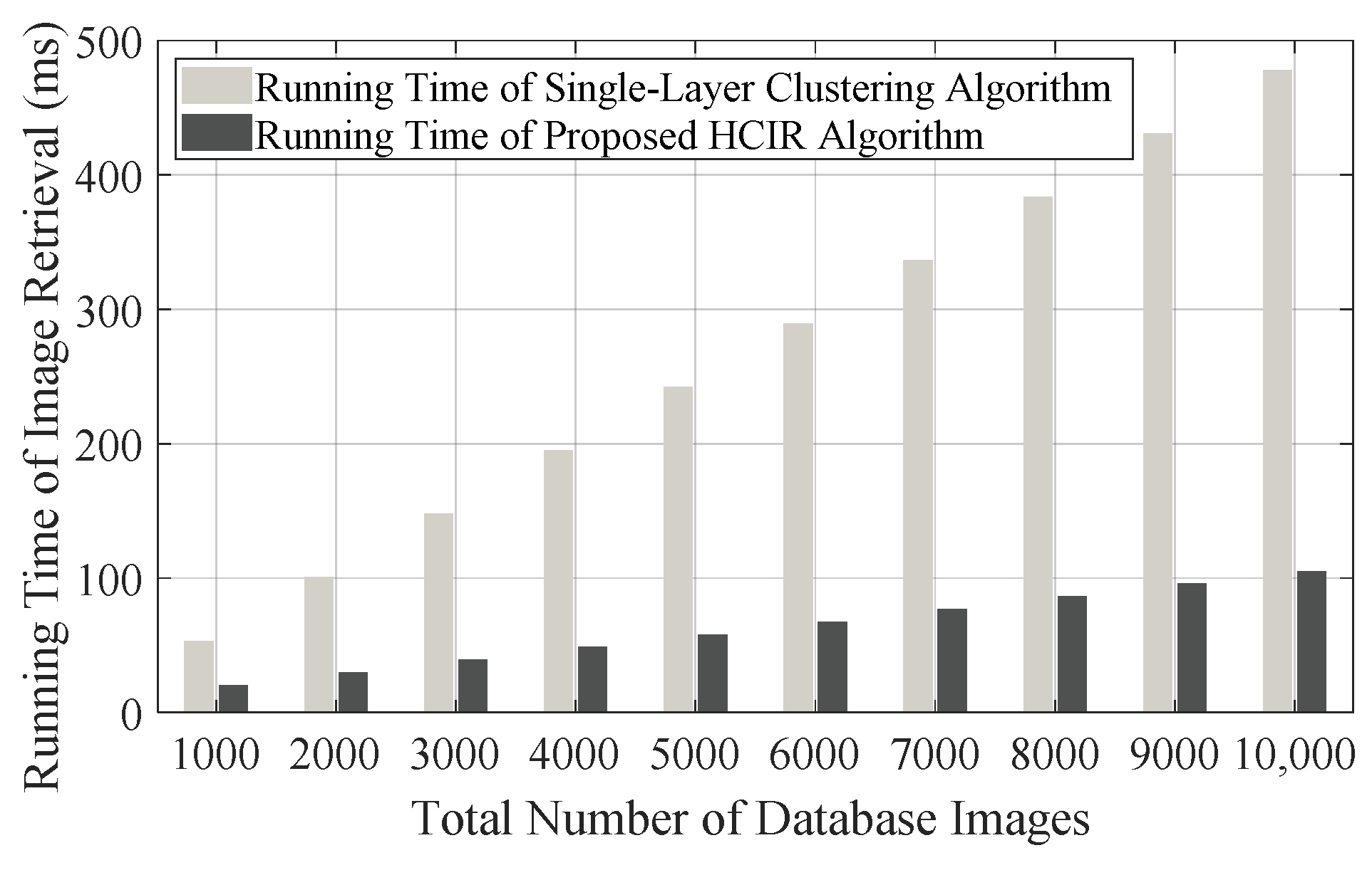
To reveal the performance difference between the single-layer clustering algorithm and the proposed HCIR algorithm, there are ten indoor scenes used for simulation, and
is separately set as 100, 200, 400, 800, and 1000, and then the running time of image retrieval for different database sizes can be simulated, as shown in
Figure 11. As a pre-condition of simulation, the backtracking mechanism is always not triggered. According to the simulation results, the advantage of the proposed algorithm is that the running time does not linearly increase along with the growth of the database size. Even when the database image size is increased to 10,000, the running time of image retrieval is less than 110 ms. In this case, the running time of image retrieval corresponding to the single-layer clustering-based algorithm almost reaches 500 ms, which means that only two retrievals can be performed per second. In contrast, by the proposed HCIR algorithm, image retrieval can be executed nine times when there are 10,000 images in the database. The reason that the proposed algorithm spends less time coping with image retrieval is that database images are reasonably grouped in the off-line stage. Furthermore, on a deeper level, time for image clustering is sacrificed in the off-line stage to reduce the time consumption of image retrieval in the on-line stage.
To demonstrate the performance of the proposed WKNN algorithm, two typical image retrieval-based localization methods (i.e., the NN method [
49,
54,
55] and the KNN method [
56,
57]) are selected and implemented. Each image in the KTH database and the HIT-TUM database is employed as a query image for visual localization. For the proposed WKNN method and the typical KNN method, five nearest neighbors are selected to estimate the query position [
57]. In order to reveal the impact of image acquisition intervals (
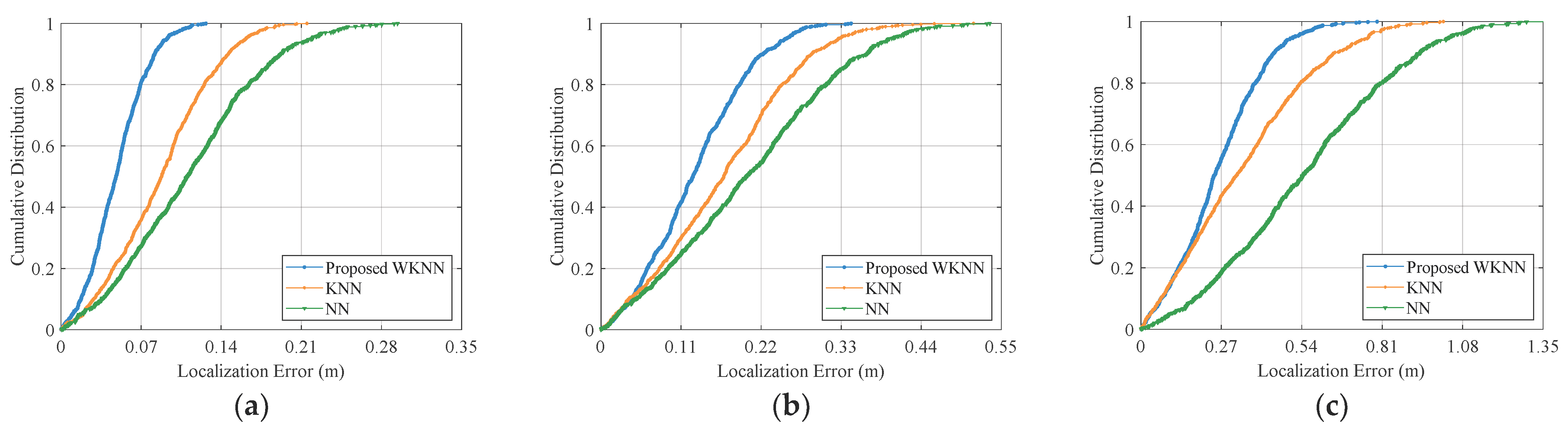
din) on localization accuracy, database images with different acquisition intervals are set for experiments. Localization errors of query images are calculated, and the cumulative distributions of the errors are shown in
Figure 12.
To quantitatively analyze the performance improvement of the WKNN method, an accuracy improvement rate
rim is introduced and defined as:
where
and
are the average errors by the proposed WKNN method and the comparative method, respectively.
Compared with the NN and KNN methods, the proposed WKNN method achieves a better performance on localization accuracy, as shown in
Table 8. In all experimental cases, the improvement of average localization accuracy reaches at least 22% and 34%, respectively, compared with the KNN and NN methods. From the localization results, it can be found that when the database images are more densely captured, the advantage of the proposed method in terms of localization accuracy is more obvious compared with the two other localization methods. The reason is that when the intervals of database images are large, the common visual features between the query image and the database images are few, which weakens the contributions of the weights in the WKNN method.
As illustrated in
Table 8, when the database image acquisition intervals are set to be 10 cm, 20 cm, 30 cm, 40 cm, and 50 cm, the average localization errors of the WKNN method are 0.0490 m, 0.1299 m, 0.2604 m, 0.3673 m, and 0.5048 m, respectively. The results indicate that localization accuracy increases along with database image acquisition intervals. Even if the acquisition interval is increased to 50 cm, the sub-meter localization accuracy can be achieved by the proposed method, which satisfies the requirements of most indoor location-based services. But it is worth noting that acquisition intervals that are too small lead to a large off-line image database and result further in a high time overhead of image retrieval. Therefore, when designing a visual indoor localization system, a proper database image acquisition interval should be selected by striking a balance between localization accuracy and efficiency.


