
Research on Path-Planning Algorithm Integrating Optimization A-Star Algorithm and Artificial Potential Field Method


Abstract
:1. Introduction
2. Global Path Planning
2.1. Traditional A-Star Algorithm
2.2. Optimization of the A-Star Algorithm
3. Local Route Planning
3.1. Artificial Potential Field Method
3.2. Optimization of the Artificial Potential Field Method
3.2.1. Interruption Point Selection
3.2.2. Least Squares Method
4. Simulation and Analysis
4.1. Comparative Analysis of Optimization Algorithms and Traditional Algorithms
4.2. Comparative Analysis of Optimized A-Star Algorithm and Bidirectional A-Star Algorithm
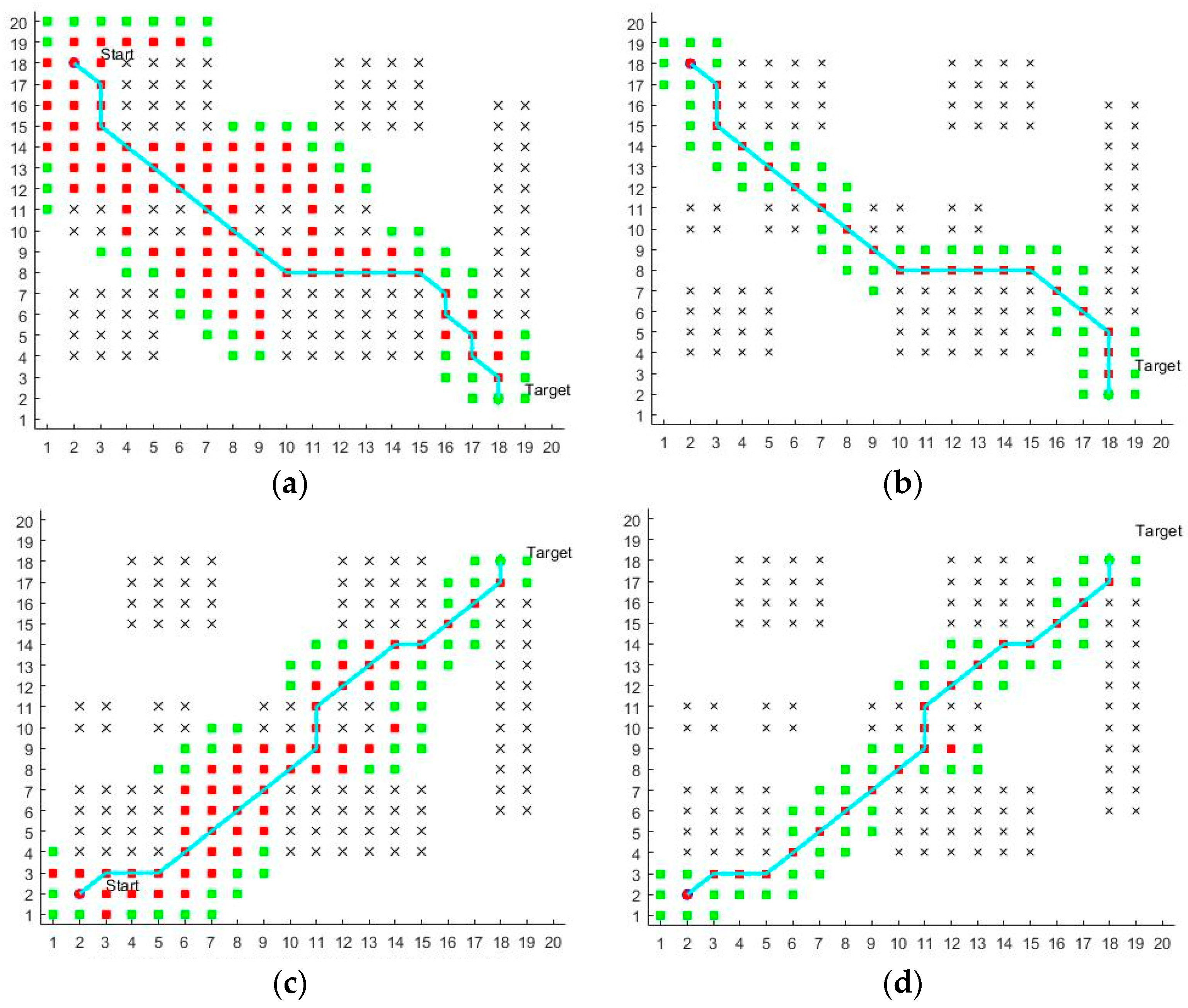
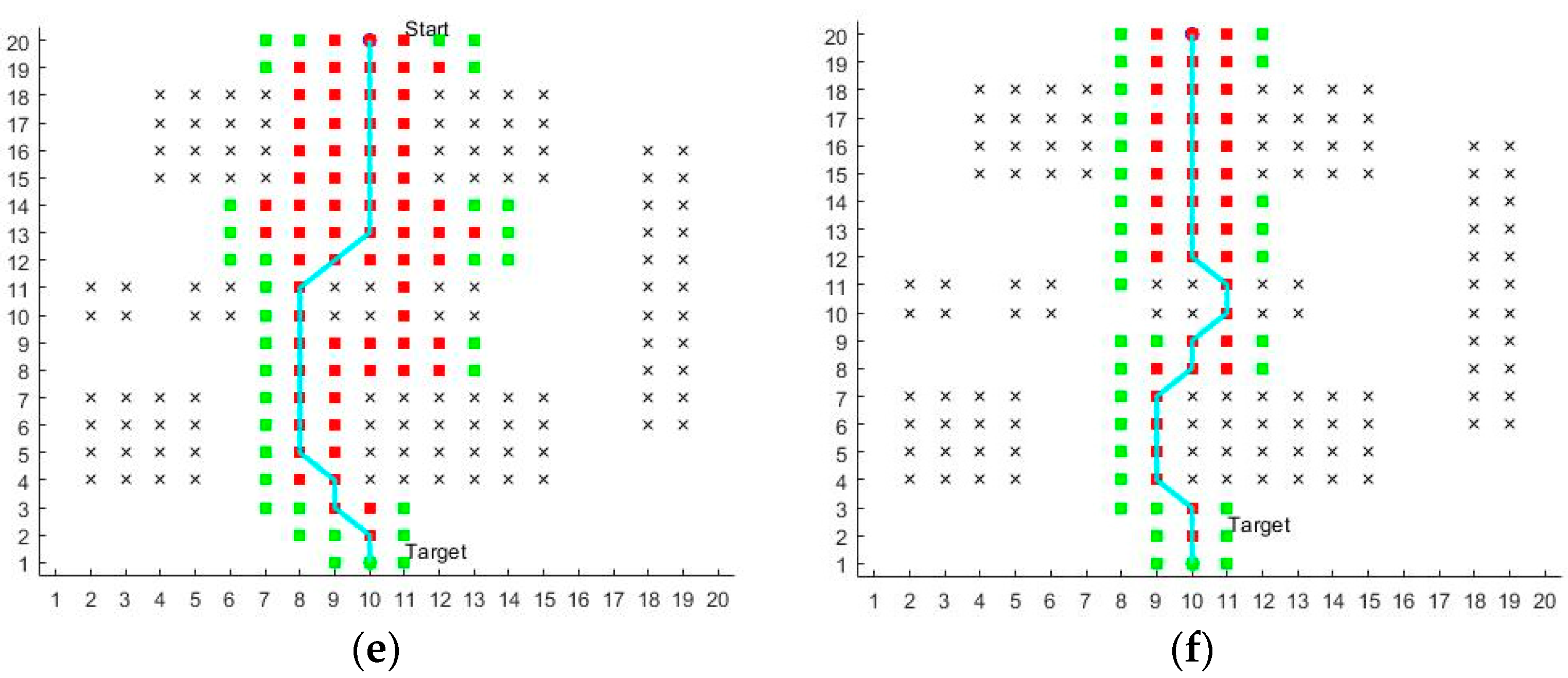
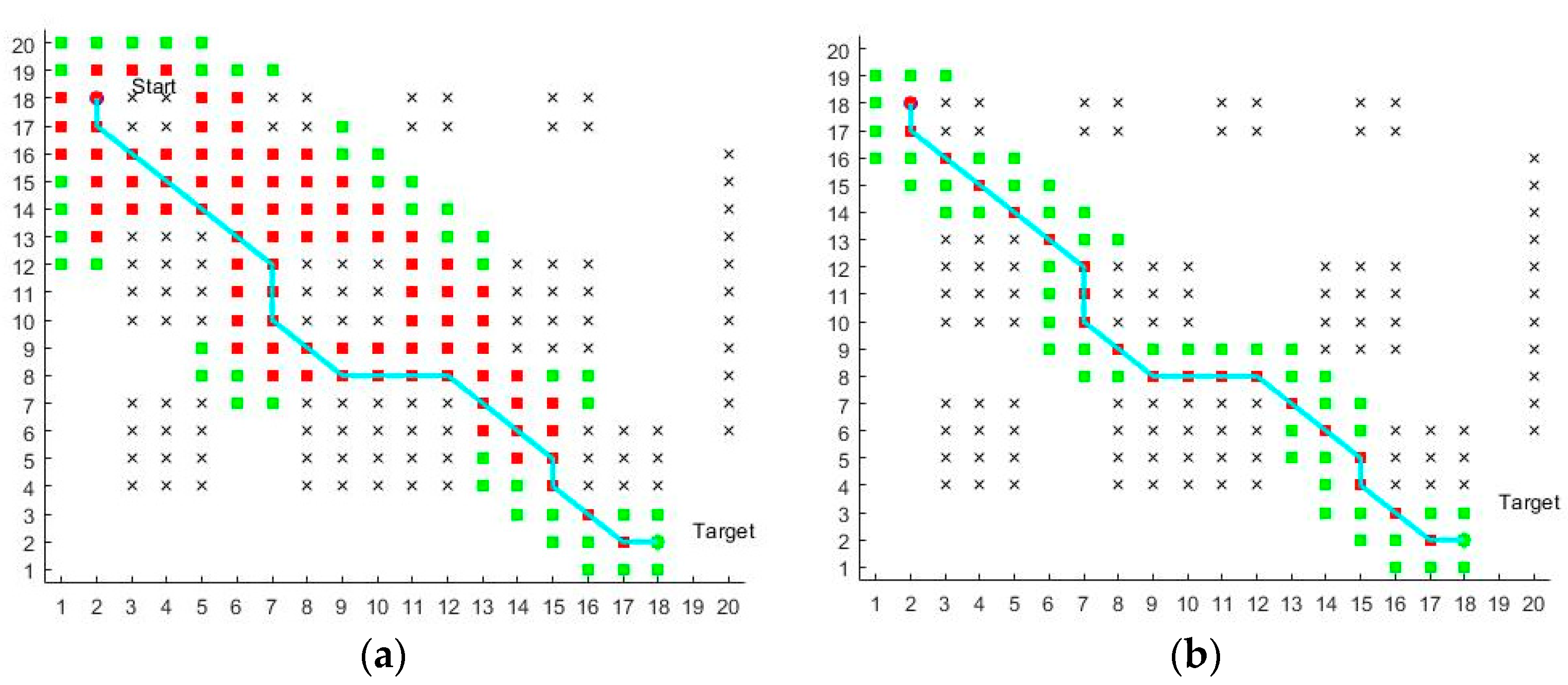
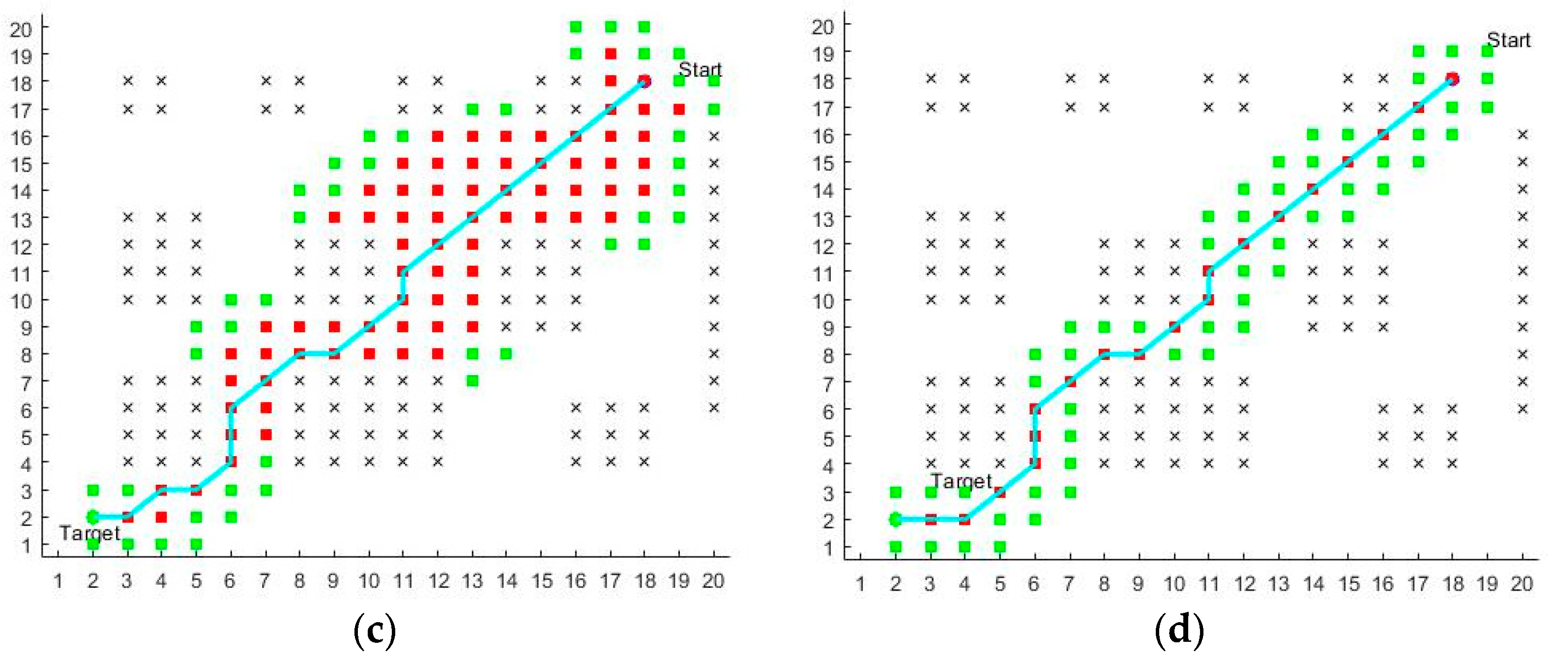
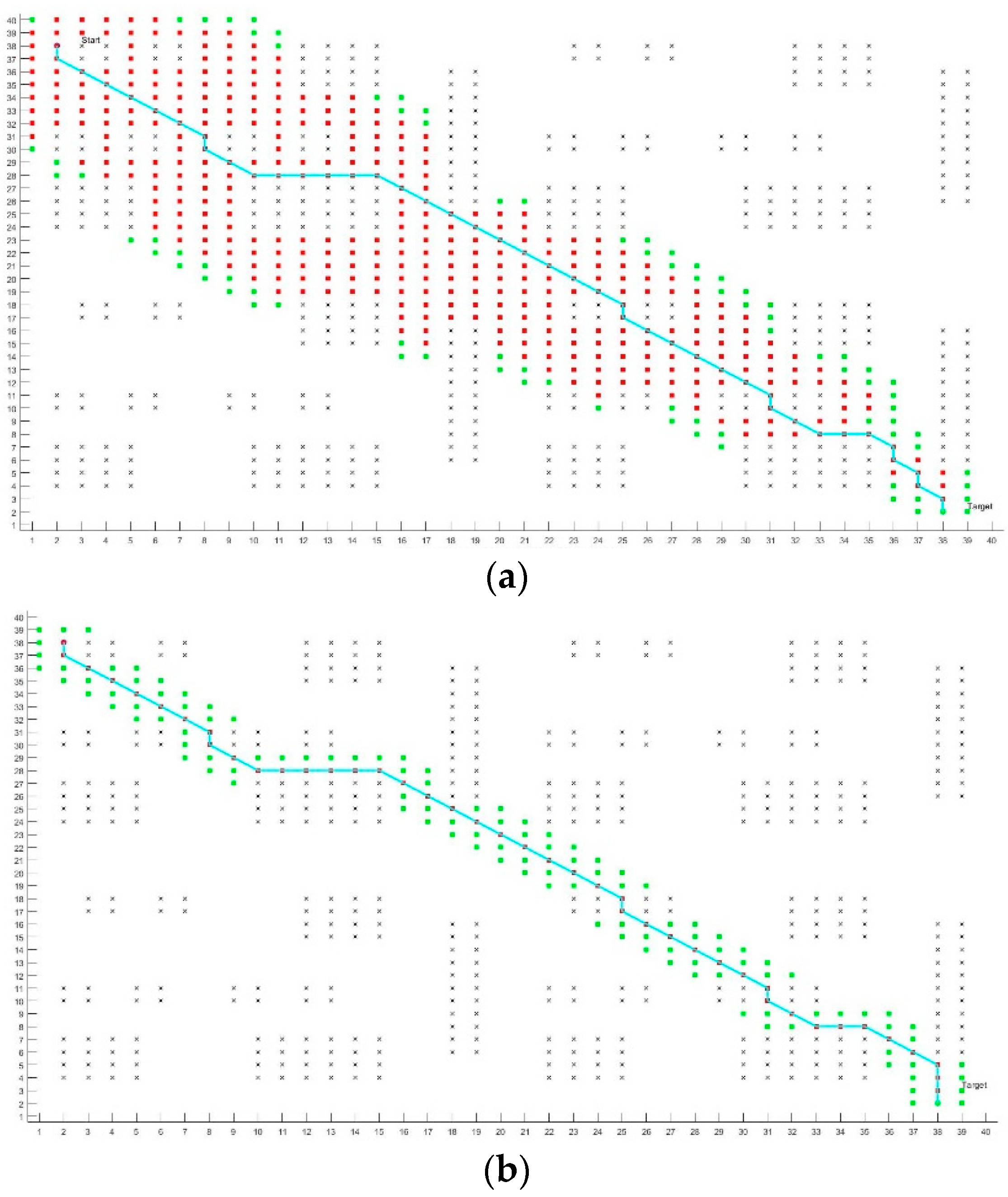
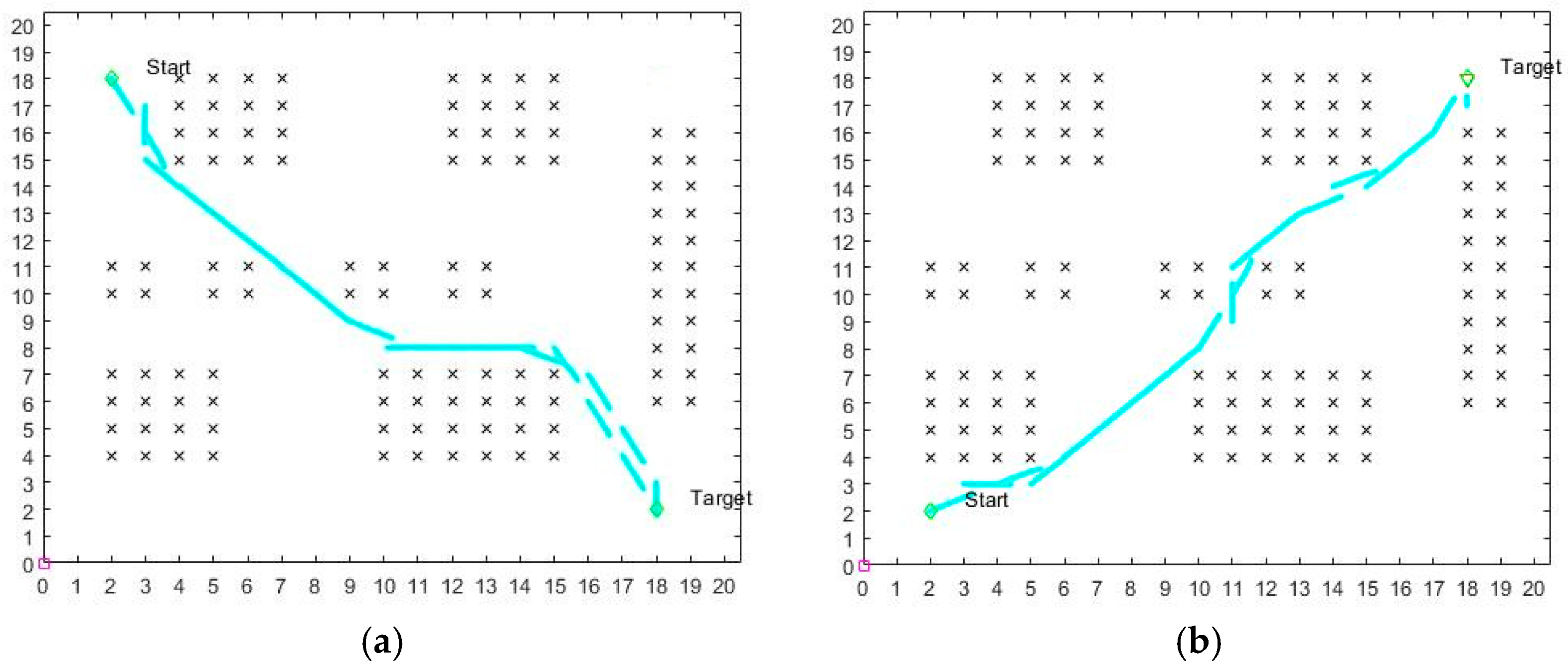
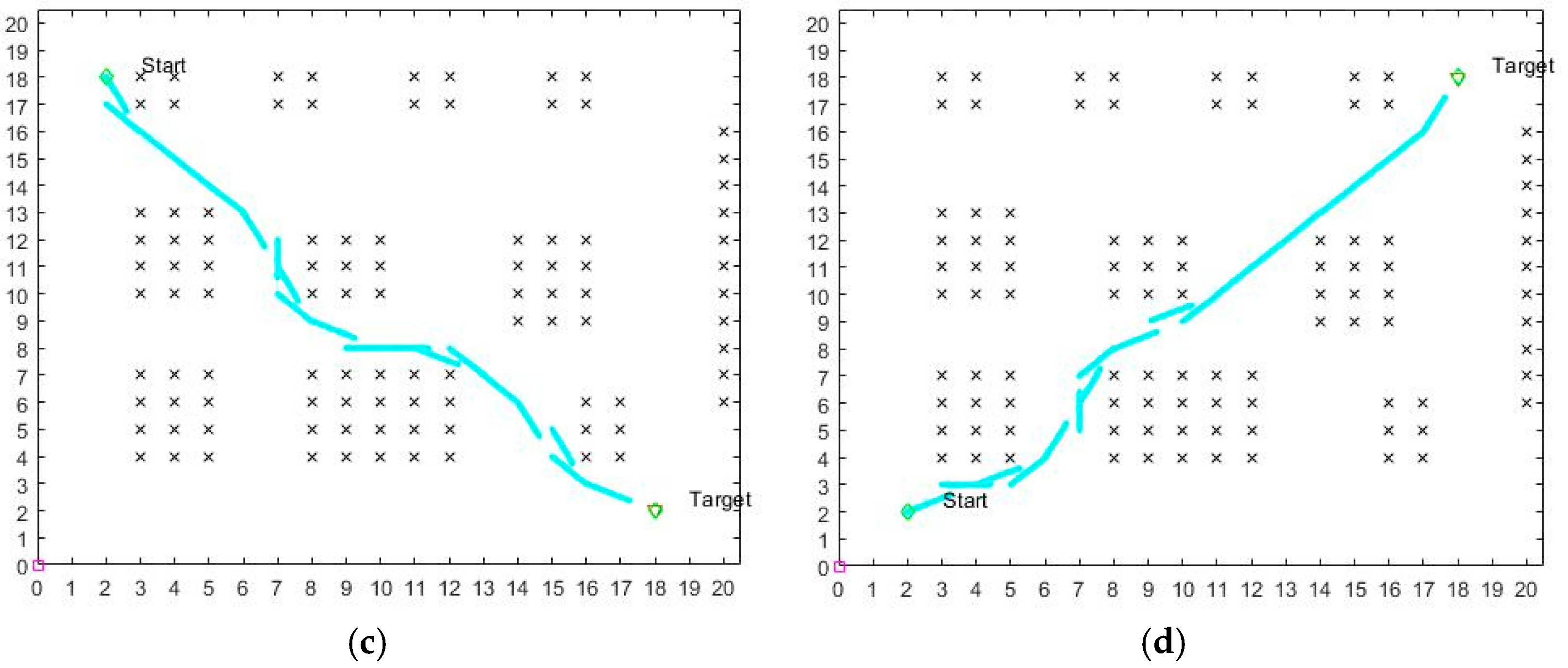
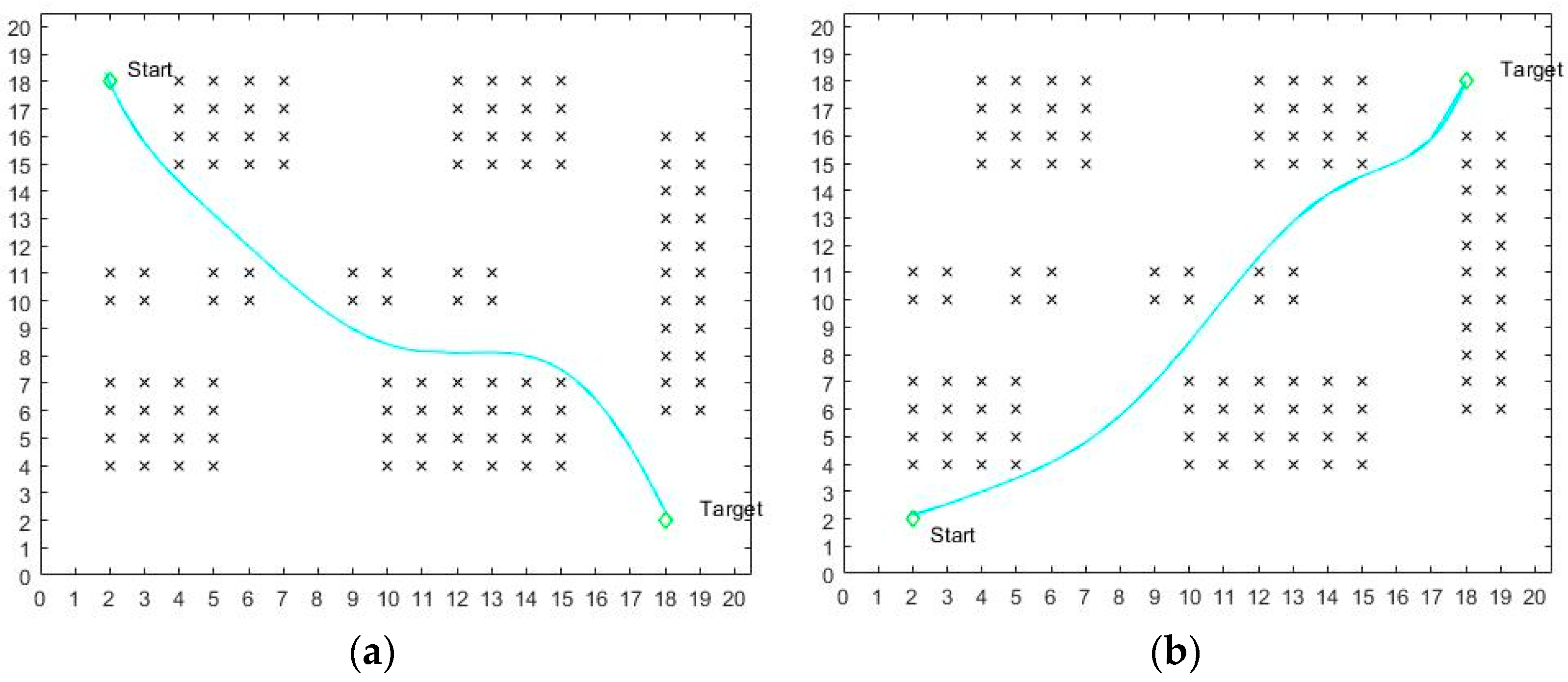
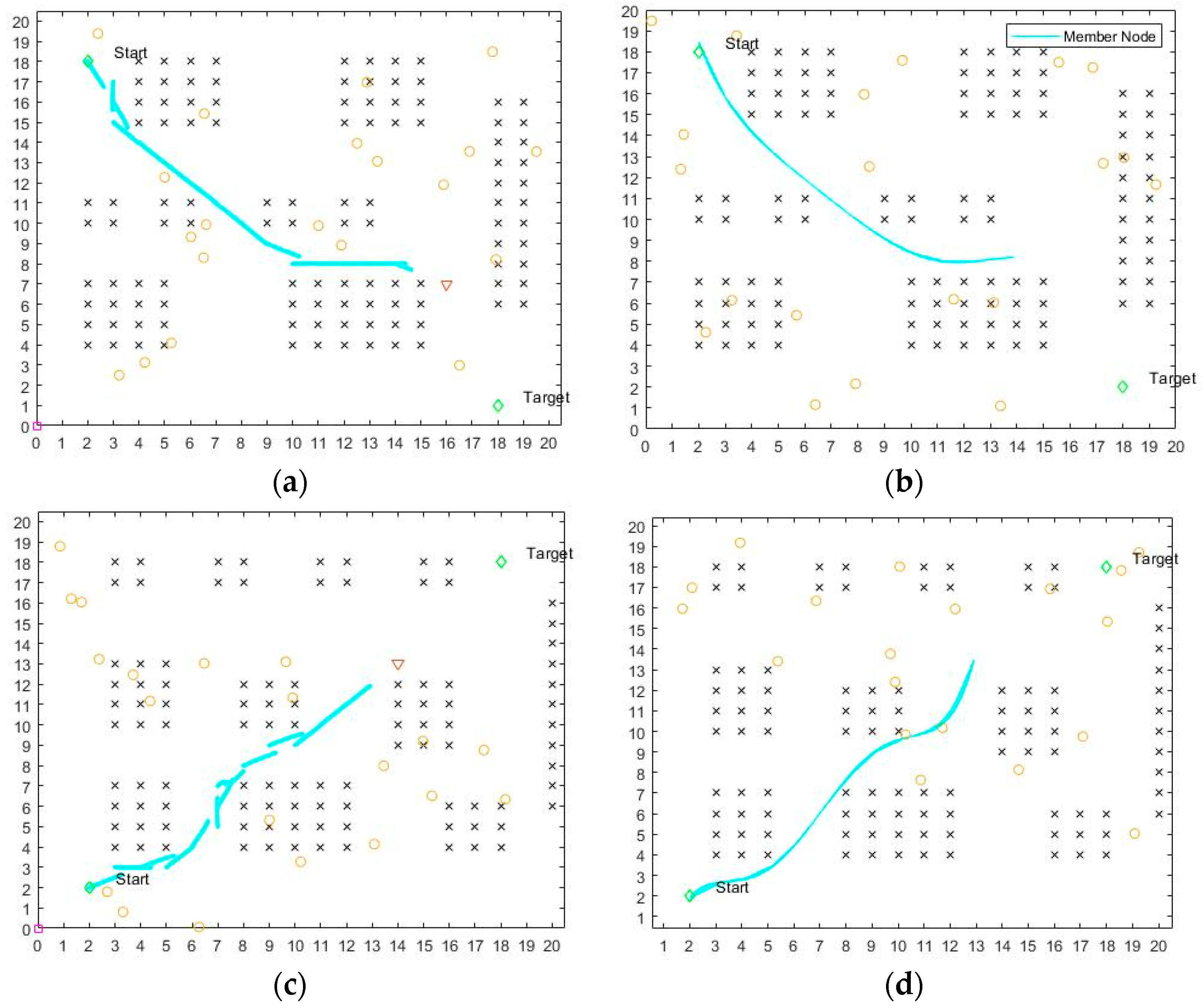
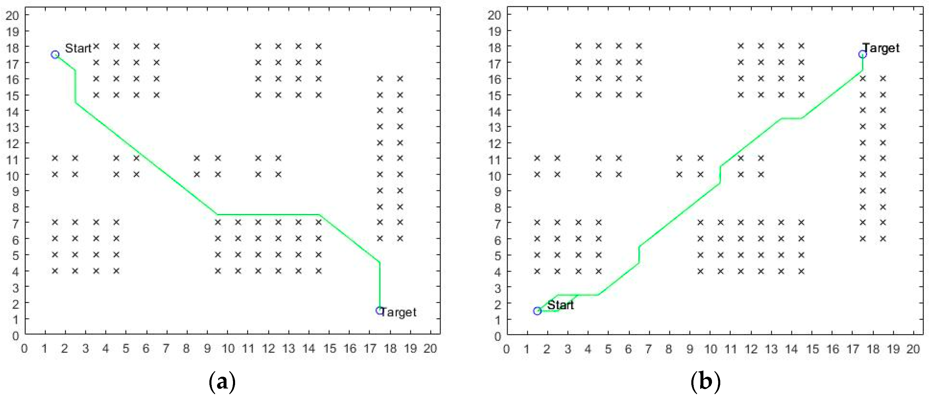
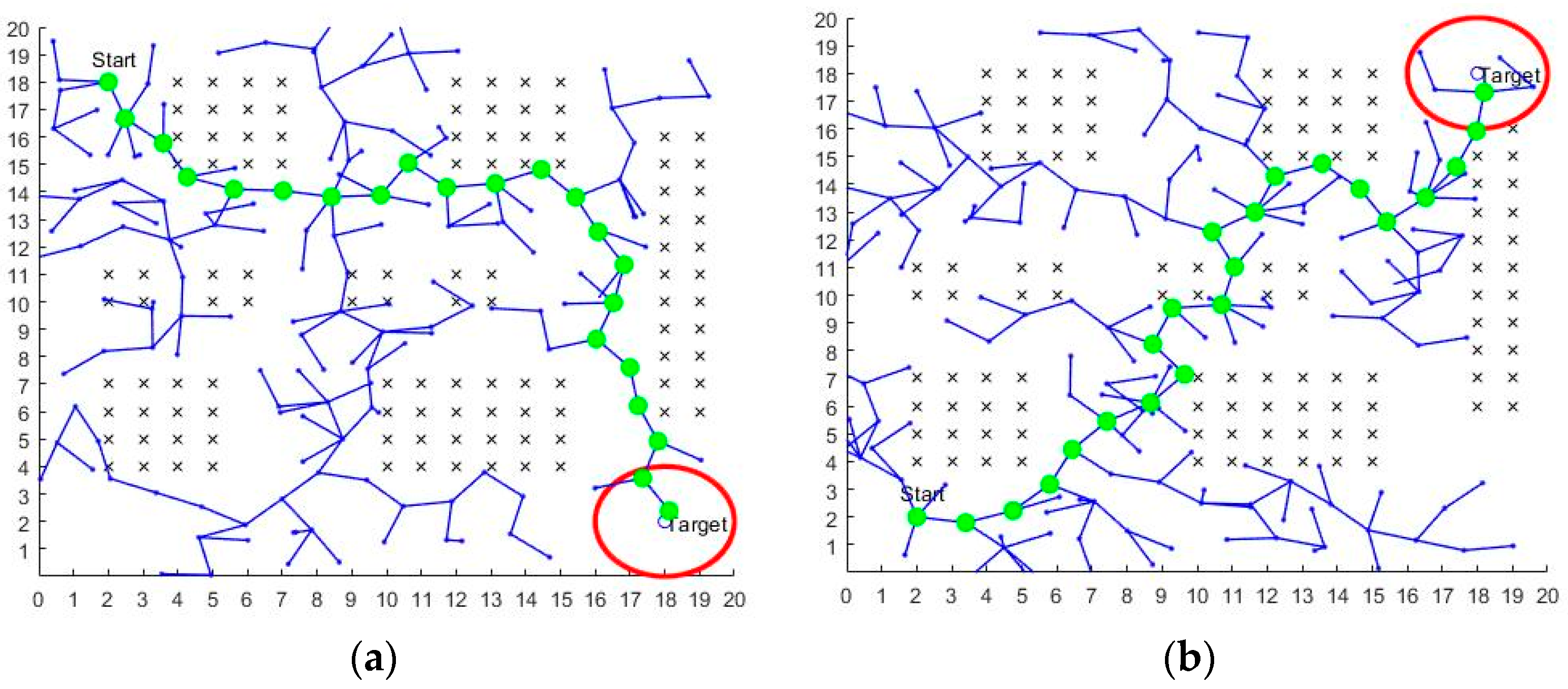
 ” in the diagram. A comparison of the path planning of the optimized A-star algorithm and the bidirectional A-star algorithm proposed in this paper shows that the optimized A-star algorithm has better throughput, that the path-planning efficiency of the optimized A-star algorithm is higher (as shown in Table 4), and that the path-planning time of the optimized A-star algorithm is 65.2% less than the path-planning time of the bidirectional A-star algorithm. The number of computing nodes is 103 in Figure 14a and 70 in Figure 14b. The optimized A-star algorithm reduces the number of computing nodes by approximately 32% compared to the bidirectional A-star algorithm. Meanwhile, as shown in Figure 14a,c, the bidirectional A-star algorithm is affected by various factors such as obstacle size and map environment complexity when selecting virtual endpoints, which indirectly affects the pathfinding efficiency of the bidirectional A-star algorithm. The pathfinding efficiency of the optimized A-star algorithm is only affected by the complexity of the map environment, and therefore the performance of the optimized A-star algorithm is more stable than that of the bidirectional A-star algorithm.
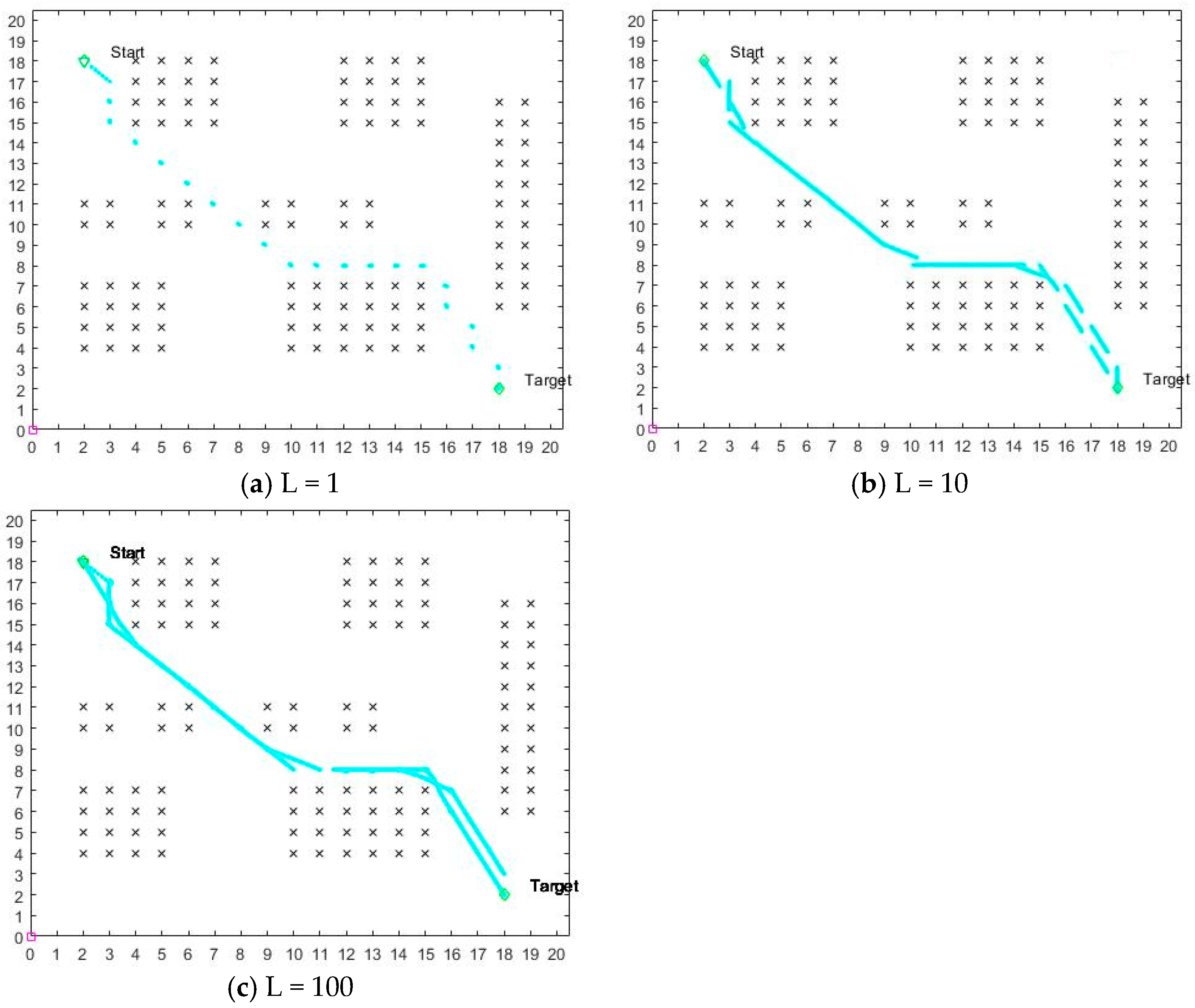
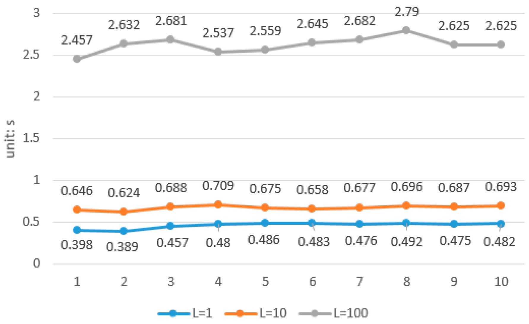
4.3. Simulation Analysis of the Effect of Different L Values on the Potential Field Method
4.4. Comparative Analysis of Fusion and Ant Colony Algorithms
4.5. Comparative Analysis of Fusion Algorithms and the RRT Algorithm
5. Results and Discussion
6. Conclusions
Author Contributions
Funding
Acknowledgments
Conflicts of Interest
References
- Liu, J.; Zhang, L.; Li, H. The study on path planning of stair cleaning robot rest platform. J. Jiangxi Norm. Univ. (Nat. Sci.) 2022, 46, 67–74. [Google Scholar]
- Yang, M.; Xie, M.; Zhang, X. The Design of Obstacle Avoidance System and Path Planning of Cleaning Robot. Chang. Inf. Commun. 2021, 34, 14–17. [Google Scholar]
- Li, X.; Ma, X.; Wang, X. A Survey of Path Planning Algorithms for Mobile Robots. Comput. Meas. Control 2022, 30, 9–19. [Google Scholar]
- Zhang, K. Overview of Path Planning Algorithms for Unmanned Vehicles. Equip. Manuf. Technol. 2021, 6, 111–113. [Google Scholar] [CrossRef]
- Yang, Y. Overview of Global Path Planning Algorithms for Mobile Robots. Inf. Rec. Mater. 2022, 23, 29–32. [Google Scholar]
- Wang, Z.; Hu, X.; Li, X.; Du, Z. Overview of Global Path Planning Algorithms for Mobile Robots. Comput. Sci. 2021, 48, 19–29. [Google Scholar]
- Dijkstra, E. A Note on Two Problems in Connexion With Graphs. In Numerische Mathematik; Springer: New York, NY, USA, 1959; pp. 269–271. [Google Scholar]
- Hart, P.E.; Nilsson, N.J.; Raphael, B. A formal basis for the heuristic determination of minimum cost paths in graphs. IEEE Trans. Syst. Sci. Cybern. 1968, 4, 100–107. [Google Scholar] [CrossRef]
- Zhang, X.; Zou, Y. Collision-free path planning for automated guided vehicles based on improved A-star algorithm. Syst. Eng. Theory Pract. 2021, 41, 240–246. [Google Scholar]
- Khatib, O. The Potential Field Approach and Operational Space Formulation in Robot Control; Springer: New York, NY, USA, 1986; pp. 367–377. [Google Scholar]
- Wang, Y. Improvement of Artificial Potential Field Algorithm for Robots in Different Environments. Nanjing Univ. Inf. Sci. Technol. 2020, 2, 45–53. [Google Scholar]
- Liu, H.; Wang, D.; Wang, Y.; Lu, X. Research of Path Planning for Mobile Robots Based on Fuzzy Artificial Potential Field Method. Control Eng. China 2022, 29, 33–38. [Google Scholar]
- Sheng, L.; Bao, L.; Wu, P. Application of Heuristic Approaches in the Robot Path Planning and Optimization: A Review. Electron. Opt. Control 2018, 25, 58–64. [Google Scholar]
- Hen, J.; Wen, J.; Xie, G. Mobile robot path planning based on improved A-star algorithm. J. Guangxi Univ. Sci. Technol. 2022, 33, 78–84. [Google Scholar]
- Lin, M.; Yuan, K.; Shi, C.; Wang, Y. Path planning of Mobile robot based on improved A-star algorithm. Mech. Sci. Technol. Aerosp. Eng. 2022, 41, 795–800. [Google Scholar]
- Zhou, J.; Yang, L.; Zhang, C. Indoor robot path planning based on improved A-star algorithm. Mod. Electron. Tech. 2022, 32, 202–206. [Google Scholar]
- Shi, Z.; Mei, S.; Shao, Y.; Wan, R.; Song, Z.; Xie, M.; Li, Y. Research status and prospect of path planning for mobile robots based on artificial potential field method. J. Chin. Agric. Mech. 2022, 42, 182–188. [Google Scholar]
- Liu, X. Review on UAV obstacle avoidance methods. J. Ordnance Equip. Eng. 2022, 43, 40–47. [Google Scholar]
- Wu, Q.; Zeng, Q.; Luo, J.; Kuang, X.; Huang, H. Application research on improved artificial potential field method in UAV path planning. J. Chongqing Univ. Technol. (Nat. Sci.) 2022, 36, 144–151. [Google Scholar]
- Sun, L. Obstacle Avoidance Algorithm of Autonomous Vehicle Based on an Improved Artificial Potential Field. J. Henan Univ. Sci. Technol. (Nat. Sci.) 2022, 43, 5–6, 28–34, 41. [Google Scholar]
- Gao, Q. Research on Least Square Curve Fitting and Optimization Algorithm. Ind. Control Comput. 2021, 34, 100–101. [Google Scholar]
- Wang, R. Research of Least Square Curve Fitting and Simplified Algorithm. Sens. World 2021, 27, 8–10, 25. [Google Scholar]
- Zhao, J.; Wang, J.; Lu, Z.; Sun, H. Research on path planning of medical inspection robot based on improved bidirectional exploration A-star algorithm. J. Jilin Norm. Univ. (Nat. Sci. Ed.) 2022, 43, 121–127. [Google Scholar]
- Wang, Z.; Zeng, G.; Huang, B. Mobile robot path planning algorithm based on improved bidirectional A star. Transducer Microsyst. Technol. 2020, 39, 141–143, 147. [Google Scholar]
- Yue, G.; Zhang, M.; Shen, C.; Guan, X. Bi-directional smooth A-star algorithm for navigation planning of mobile robots. Sci. Sin. Technol. 2021, 51, 459–468. [Google Scholar] [CrossRef]
- Chen, D.; Liu, X.; Liu, S. Improved A-star algorithm based on two-way search for path planning of automated guided vehicle. J. Comput. Appl. 2021, 41, 309–313. [Google Scholar]
- Wang, Z.; Xia, X. Application of adaptive ant colony algorithm in robot path planning. J. Minnan Norm. Univ. (Nat. Sci.) 2022, 35, 38–45. [Google Scholar]
- Yue, C.; Huang, J.; Deng, L. Research on improved ant colony algorithm in AGV path planning. Comput. Eng. Des. 2022, 43, 2533–2541. [Google Scholar]
- Wang, H.; Cui, Y.; Li, M.; Li, G. Mobile Robot Path Planning Algorithm Based on Improved RRT∗FN. J. Northeast Univ. (Nat. Sci.) 2022, 43, 1217–1224, 1249. [Google Scholar]
- Chen, H.; Wang, L. A Path Planning Algorithm Based on Two-Way Simultaneous No-Collision Goal RRT. J. Airf. Eng. Univ. (Nat. Sci. Ed.) 2022, 23, 60–67. [Google Scholar]


| Time | 1 | 2 | 3 | 4 | 5 | 6 | 7 | 8 | 9 | 10 |
|---|---|---|---|---|---|---|---|---|---|---|
| Traditional A-star algorithm | 0.623 | 0.583 | 0.635 | 0.592 | 0.606 | 0.581 | 0.604 | 0.600 | 0.596 | 0.603 |
| Optimization of the A-star algorithm | 0.368 | 0.225 | 0.208 | 0.190 | 0.218 | 0.175 | 0.179 | 0.172 | 0.170 | 0.174 |
| Time | 1 | 2 | 3 | 4 | 5 | 6 | 7 | 8 | 9 | 10 |
|---|---|---|---|---|---|---|---|---|---|---|
| Traditional A-star algorithm | 0.309 | 0.307 | 0.308 | 0.305 | 0.303 | 0.299 | 0.304 | 0.300 | 0.296 | 0.299 |
| Optimization of the A-star algorithm | 0.140 | 0.139 | 0.139 | 0.139 | 0.140 | 0.138 | 0.136 | 0.134 | 0.133 | 0.133 |
| Time | 1 | 2 | 3 | 4 | 5 | 6 | 7 | 8 | 9 | 10 |
|---|---|---|---|---|---|---|---|---|---|---|
| Traditional A-star algorithm | 2.427 | 2.436 | 2.419 | 2.371 | 2.402 | 2.552 | 2.349 | 2.359 | 2.371 | 2.368 |
| Optimization of the A-star algorithm | 0.683 | 0.732 | 0.703 | 0.689 | 0.691 | 0.782 | 0.704 | 0.699 | 0.685 | 0.692 |
| Time | 1 | 2 | 3 | 4 | 5 | 6 | 7 | 8 | 9 | 10 |
|---|---|---|---|---|---|---|---|---|---|---|
| Two-way exploration A-star algorithm | 0.486 | 0.493 | 0.497 | 0.452 | 0.462 | 0.489 | 0.473 | 0.472 | 0.458 | 0.454 |
| Optimization of the A-star algorithm | 0.163 | 0.157 | 0.161 | 0.158 | 0.154 | 0.162 | 0.169 | 0.181 | 0.183 | 0.158 |
| Time | 1 | 2 | 3 | 4 | 5 | 6 | 7 | 8 | 9 | 10 |
|---|---|---|---|---|---|---|---|---|---|---|
| Ant colony algorithm | 2.185 | 2.092 | 2.029 | 2.047 | 2.053 | 2.064 | 2.066 | 2.049 | 2.055 | 2.092 |
| Fusion algorithm | 0.693 | 0.712 | 0.706 | 0.718 | 0.700 | 0.750 | 0.740 | 0.736 | 0.738 | 0.726 |
Publisher’s Note: MDPI stays neutral with regard to jurisdictional claims in published maps and institutional affiliations. |
© 2022 by the authors. Licensee MDPI, Basel, Switzerland. This article is an open access article distributed under the terms and conditions of the Creative Commons Attribution (CC BY) license (https://creativecommons.org/licenses/by/4.0/).
Share and Cite
Liu, L.; Wang, B.; Xu, H. Research on Path-Planning Algorithm Integrating Optimization A-Star Algorithm and Artificial Potential Field Method. Electronics 2022, 11, 3660. https://doi.org/10.3390/electronics11223660
Liu L, Wang B, Xu H. Research on Path-Planning Algorithm Integrating Optimization A-Star Algorithm and Artificial Potential Field Method. Electronics. 2022; 11(22):3660. https://doi.org/10.3390/electronics11223660
Chicago/Turabian StyleLiu, Lisang, Bin Wang, and Hui Xu. 2022. "Research on Path-Planning Algorithm Integrating Optimization A-Star Algorithm and Artificial Potential Field Method" Electronics 11, no. 22: 3660. https://doi.org/10.3390/electronics11223660