Propagation Channel Characterization for 6–14 GHz Bands Based on Large Array Measurement for Indoor Scenarios

Abstract

The demand for wideband data transmission in the “next-generation” mobile communication system is growing rapidly. As the frequency band around 10 GHz could be the option for 6th-generation (6G) wireless communication systems. In this paper, a recently conducted measurement campaign in the 6–14 GHz radio wave propagation channel using a large antenna array with 1024 elements is introduced. In order to investigate the behavior of the wideband channel, we have analyzed the channel characteristics with respect to different carrier frequencies, bandwidths, the locations of antenna elements, and user locations, aiming at exploring the spatio-frequency variability of channels in the massive multiple-input multiple-output (MIMO) scenarios. Moreover, the sparsity of the channel in frequency and spatial domains is evaluated through the degree of freedom (DoF) analysis, and statistical models are established.

1. Introduction

As 5th-generation (5G) mobile communication technology has been put into commercial use globally, wideband transmission technology is getting more popular with the features of a higher rate and lower latency in data transmission. Previous research mainly focused on narrow-band channels with bandwidth less than 1 GHz. For example, the bandwidth of 5G systems allocated to 3 major operators in China for commercial use is 100 MHz. With such limited bandwidth, the wideband transmission is eager to be promoted. Against this background, 6th-generation (6G) wireless systems are proposed with large uplink broadband capacity, low latency, and high frequency, which are supposed to be put into commercial use around 2030.

ultra-wide band (UWB) technology was specified by Federal Communications Commission (FCC) as a large spectrum with the bandwidth of more than 500 MHz in 3.1–10.6 GHz band in 2002 [1,2]. Since then, research on UWB channels have attracted extensive interests in the field of intra-vehicular wireless sensor network (IVWSN), positioning and so on [3,4]. In the 2000s, researchers were interested in large-scale fading models, path loss (PL) models, and small-scale statistics [5] for channels in time [4,6,7,8], frequency [6], and spatial [9] domains within the band declared by FCC. Nevertheless, the latest research on wideband channels have been developed with advanced technologies or fields in higher frequency bands [10,11,12] such as the multiple-input multiple-output (MIMO) systems [13], body-to-body (B2B) scenarios [13], propagation graph modeling [14], sparsity channel estimation algorithm [15], and so on.

In 2019, the world radiocomunication conference (WRC) released an agenda which will be discussed at the 2023 WRC. This agenda considers the identification of the frequency bands 3.3–10.5 GHz for International Mobile Telecommunications (IMT) [16] and suggests that the potential spectrum for 6G systems might be around 10 GHz and specific band in sub-THz band (275–450 GHz) [17] for multi-band collaboration technology. However, the attractive frequency bands for researchers were sub-6 GHz for 5G systems [18,19], millimeter-wave (mm-Wave) mainly for outdoor time-varying vehicle to everything (V2X) communications [20,21,22], and sub-THz [10,11,12] for potential 6G systems with a blank at around 10 GHz.

In conclusion, previous research for UWB channels around 10 GHz were conducted in the 2000s with unadvanced equipment or research methods, while recent wideband channel explorations focus on sub-6 GHz or higher frequency bands using well-developed technologies and methods. On the other hand, the above studies explored the statistical models for large- and small-scale fading parameters of UWB channels in conventional domains in either line-of-sight (LoS) or non-line-of-sight (NLoS) scenarios at around 10 GHz. However, few studies have described the channel characteristics or models from the perspectives of carrier frequency, bandwidth, multi-user (MU) locations, and receiving antenna elements. In particular, MU locations in MIMO systems are important for achieving a tera-bps transmission rate, especially in the context of 6G wireless communication systems. Therefore, to have a clear understanding of the wideband channel behaviors in the above novel dimensions in potential 6G systems, measurement-based study around 10 GHz is necessary.

In this paper, considering that the carrier frequency and bandwidth for ‘next generation’ mobile communication systems are more prominent, we perform a measurement-based research in the 6–14 GHz band channel using a large virtual antenna array with elements of $32\times 32$. The characteristics of the channel are observed in the aspects of power delay profile (PDP), degree of freedom (DoF), root mean square (RMS) delay spread and K-Factor. The validation of these characteristics with respect to different carrier frequencies, bandwidths, and spatial information for receiving antenna elements are introduced. The consistency and variability of the wideband channels are illustrated both quantitatively and qualitatively, with corresponding small-scale wideband and statistical models established.

The main contributions of this paper are described as follows:

• A systematic measurement in the indoor scenario is conducted with bandwidth of 8 GHz from 6 GHz to 14 GHz.
• Analyses of channel characteristics are conducted with respect to varying bandwidth and carrier frequency. Statistical models were proposed to describe the changes of the channel characteristics.
• In spatial domain, the variations of the wideband channel are observed with regards to different receiving antenna elements and MU locations.
• The sparsity of the channel is discussed by analyzing the DoF in frequency domain.

The structure of the paper is organized as follows: Section 2 introduces the measurement system and describes the scenario. Section 3 analyzes the characteristics of the channel in different domains. Section 4 illustrates the variation trend for the analyzed characteristics by statistical parameters and proposes statistical models describing the channel behavior. Finally, Section 5 concludes the paper.

2. Measurement Configurations

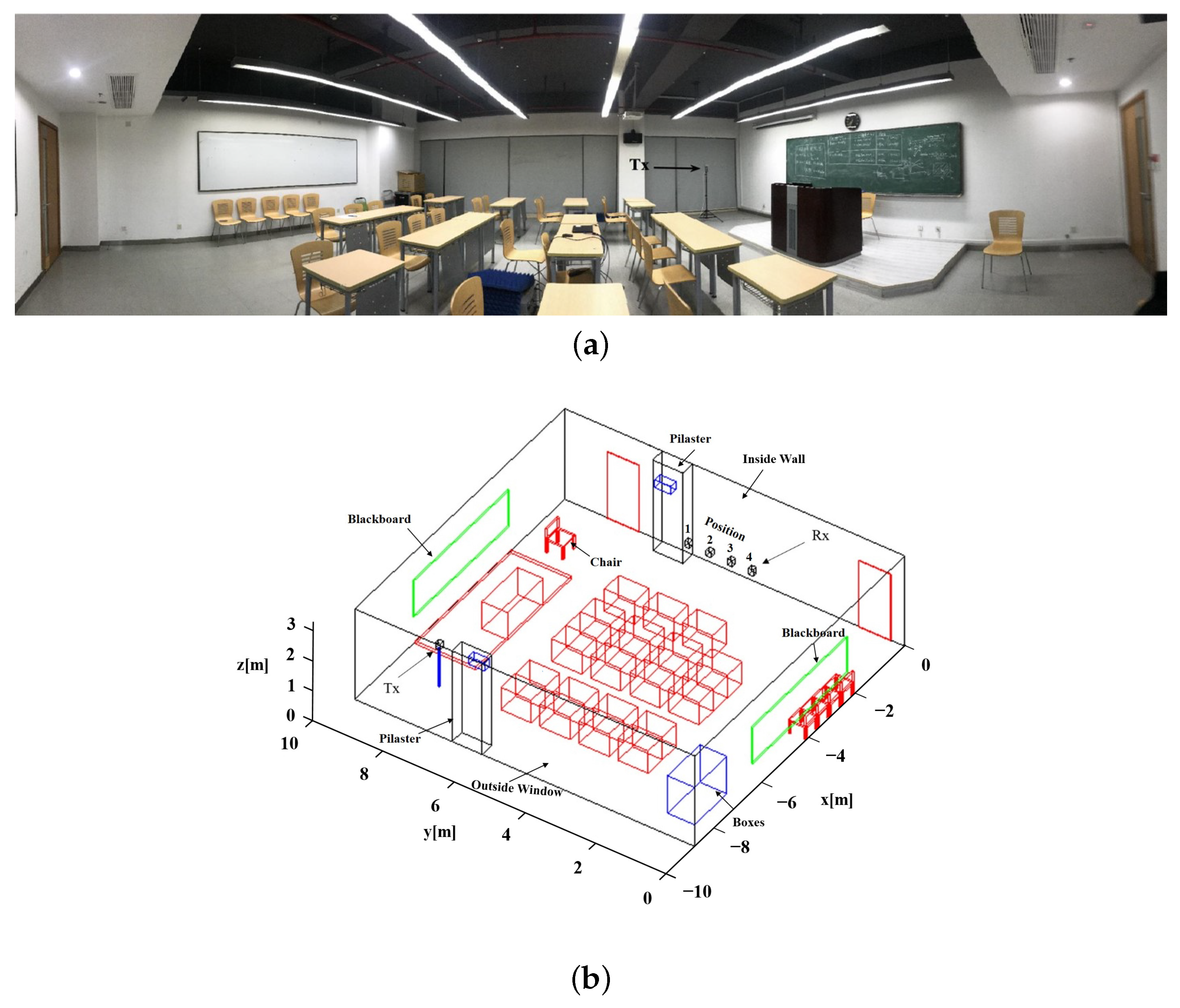
2.1. Indoor Measurement Environment

The measurement campaign was conducted in a classroom at Tongji University with the total size of $8.84\times 9.60\times 2.95$ [m${}^3$], of which the photo from the receiver (Rx) end and three dimensional (3D) digital map are described in Figure 1. In the typical classroom scenario, there are four rows of desks and chairs with the height of around 1 m. In the front and back of the classroom, there are two blackboards with different surface roughness. In addition, several cardboard boxes and aluminum boxes are stacked in the corner. The transmitter (Tx) is fixed in the corner between the platform and the outside window. The Rx is moved to four different equidistant locations near the inside wall. Both the Rx and Tx are put at the height of around 1.5 m. For each Rx location, the vertically polarized antenna is fixed on a mechanical guide, and a two dimensional (2D) virtual antenna array with elements of $32\times 32$ is formed with the movement of the guide rail.

2.2. Measurement Equipment and Setup

The measurement setup is composed of a vector network analyzer (VNA), two vertically polarized antennas for two ends, respectively, a positioner in the Tx end to lift it to the height of around 1.5 m, a mechanical guide in the Rx end used to generate virtual antenna array as shown in Figure 2 and a laptop to control the instruments and save the data.

The virtual antenna array was proposed in the mid-1990s, with the original purposes of achieving high accuracy direction of arrival (DoA) estimation and improving the efficiency and freedom of array elements utilization, which is conditioned by the static scenarios and the synchronization of the signals at Tx and Rx ends. With a vertically polarized antenna fixed, the mechanical guide is moved along the route shown in Figure 2, and the virtual antenna array is generated.

Parameters for the measurement setup are summarized in

Table 1. Measurement setup and specifications.

	Parameters	Setup
Antenna	Type	Biconical antennas
	Polarization mode	Vertical polarization
	Gain [dB]	2.4–4.5
	SWR	2.0:1
Antenna array	Type	2D array
	The space between antenna elements [mm]	$10.71$
	Number of antenna elements	$32\times 32$
VNA	Frequency band [GHz]	6–14
	Frequency points	1001
	Transmitted power [dBm]	0

for three parts: antenna specifications, antenna array settings and parameters for VNA.

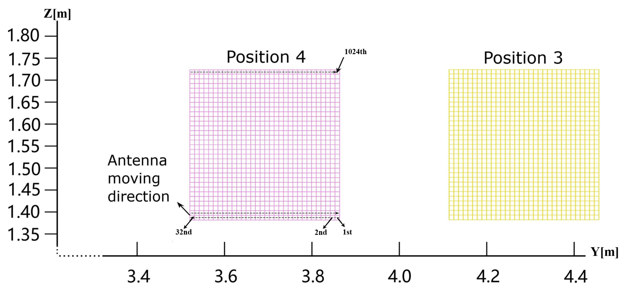
2.3. Measurement Data Description

The channel frequency response (FR) is extracted after end-to-end calibration and the channel impulse response (CIR) can be calculated by doing the inverse Fourier transformation of the channel FR. The PDP is calculated as the power gain provided by the propagation channel with respect to the delay.

As shown in Figure 3a, the shapes and values of PDP are similar in different user locations with slight lags in delay, reflecting the real spatial relationships from Tx to different Rx ends in the classroom in Figure 1b. Moreover, the distribution of multipath components (MPCs) shown in Figure 3a reveals the rich scattering effect in the indoor scenario. Figure 3b describes the variation of PDP as the virtual antenna element changes in the Rx end for one LoS path. It can be observed that the channel is selective and appears to be periodic in spatial domain. More specifically, the power changes evidently along the antenna row, while it is almost the same along the antenna column. These observations illustrate that multipath richness is more significant in the azimuthal direction than in the elevation.

3. Analysis of Characteristics for Wideband Channels in 4 Dimensions

In this section, specific characteristics, i.e., PDP, DoF, RMS delay spread and K-Factor, are discussed with regards to the carrier frequency, bandwidth, receiving antenna elements, and user locations. Qualitative analyses are conducted with the results from the four user locations, while the pictures are demonstrated in a single position to introduce similar variations. Conversely, quantitative analyses are carried out and results from all the user locations are compared to explore the variations of the small-scale fading behaviors in the complex indoor scenario.

The sparsity of the channels is evaluated in two aspects: the small amount and dispersive distribution of large-power paths in different domains. In this paper, it is validated in delay and frequency domains by PDP and DoF, respectively. The DoF in spatial domain was adopted to characterize the number of dominant eigenchannels in the MIMO systems [23,24]. As the extension to frequency domain, parameterization of sparsity for the channel is proposed as frequency degree of freedom (FDoF). It reflects the richness of MPCs and is calculated as the number of the eigenvalues of the channel at a specified threshold in thefrequency domain. The RMS delay spread is the parameterization for the variation of PDP, describing the time dispersion effect in delay, which is calculated as the normalized second-order central moment of PDP in Equation (1).

$$\begin{array}{c}{P}_m={\int }_{-\infty }^{\infty }{P}_h\left(\tau \right)d\tau \\ T_m=\frac{{\int }_{-\infty }^{\infty }{P}_h\left(\tau \right)\tau d\tau }{P_m}\\ S_{\tau }=\sqrt{\frac{{\int }_{-\infty }^{\infty }{P}_h\left(\tau \right){\tau }^{2}d\tau }{P_m}-T_m^2}\end{array}$$

(1)

where $P_m$, $T_m$, $S_{\tau }$ are the time−integrated power, mean delay, and RMS delay spread, respectively. Moreover, Rician K-Factor is the power proportion of the LoS path in the propagation channel in Equation (2), which indicates the transmission quality by evaluating the domainated paths in the propagation channel.

$$K_r=\frac{P_{LoS}}{P_{NLoS}}$$

(2)

3.1. Effect of Carrier Frequency on Channel Characteristics

The frequency selectivity of the channels is evaluated in terms of carrier frequency. The frequency responses of the channel are obtained with varying carrier frequencies over the wide band from 6 to 14 GHz. According to the PL model [25], the higher the carrier frequency, the higher the path loss. As a result, the general effect of high carrier frequency on the channel should be the rapid attenuation of the receiving power, of which the further influence will be discussed by the introduced channel characteristics in the sequel.

3.1.1. Sparsity Analysis via PDP and FDoF

Figure 4 shows the PDP with fixed bandwidth at Position 2 and Position 4. In the perspective of the different delays, the number of large-power paths are limited and distributed apart at the end with small delays, reflecting the sparsity of the channel. Besides, compared with that at Position 4, there are paths in large delays at Position 2, which indicates the rich distribution of MPCs, as described in the real environment in Figure 1—the pilaster near Position 2 results in more paths, thus causing large delays.

The power gain obtained along carrier frequency decreases regularly with similar trends, as illustrated in Figure 4c, which is, according to our conjectures, caused by the attenuation with a short wavelength according to PL model [25]. As for the periodic variation with regular spacing among minima and maxima, which reflects the severe frequency selectivity of the wideband channel, we postulate that it is caused by the constructive and destructive superposition effect of closely-spread MPCs as frequency changes.

The FDoF can be calculated as the richness of paths in the channel. The smaller the FDoF, the sparser the channel. The Y-axis in Figure 5 is the normalized eigenvalue of the eigenchannel in frequency domain. With a specified threshold of eigenvalue, the FDoF is obtained by examing the cross of the threshold lines of the eigenvalue vs. index curve. The results in Figure 5 show the negatively correlated relationship between the FDoF and carrier frequency with fixed bandwidth, reflecting the decrease in rich scattering characteristics and increase in channel sparsity at the high-frequency band.

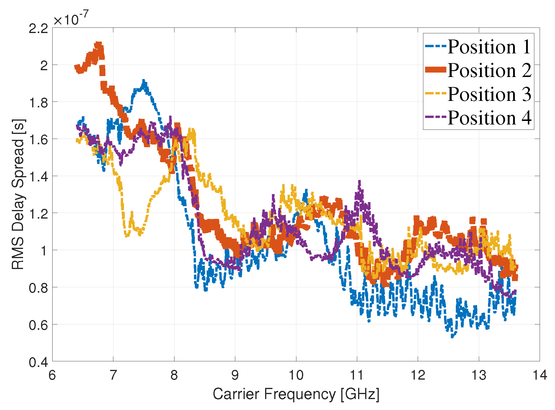
3.1.2. Frequency Selective Fading Analysis via RMS Delay Spread

With bandwidth fixed, the RMS delay spread is extracted from PDP. Figure 6 describes the decrease in the RMS delay spread on the whole with ups and downs in certain frequency bands, of which the periodic decreasing trend is similar to the results in Figure 4. It is worth mentioning that there is a sharp decline in the range of 7–9 GHz, which indicates the dramatic change in the power of the channel. The decreasing trend of the RMS delay spread with regards to the carrier frequency reflects the increase in channel sparsity along with carrier frequency, as observed in Figure 5, revealing that the attenuation of the channel is more severe at the high-frequency band.

3.1.3. Channel Fading Characteristic Analysis via K-Factor

The curves of K-Factor in Figure 7 are observed to be periodic with variations of carrier frequency similar to PDP, which is because of the constructive and destructive superposition of the MPCs according to our conjecture. Quantitatively speaking, the maximal values of K-Factor at Position 1 and Position 2 are smaller than that at Position 3 and Position 4, reflecting the rich distribution of MPCs in the environment near Position 1 and Position 2. Moreover, the values in the four locations are increasing one by one with the average values larger than 0.5, indicating that LoS paths are dominant in the channel, with the possible reason of the rich MPCs caused by the pilaster near Position 1.

3.2. Effect of Bandwidth on Channel Characteristics

The joint effect of carrier frequency and bandwidth is analyzed in this section. Theoretically, the wide band brings more ranks to the channel and thus influences the channel behaviors in all domains.

3.2.1. Sparsity Analysis via FDoF

The number of available eigenchannels is dependent on the propagation channel condition as well as the antenna array configuration for spatial degree of freedom (SDoF) [23]. Similarly, in the frequency domain, the FDoF is related to the channel condition, bandwidth and carrier frequency, as shown in Figure 5 and Figure 8. As a whole, the FDoF increases with more channel ranks caused by increasing bandwidth. Thus, the relationships between the channel sparsity and bandwidth, and that between the channel sparsity and carrier frequency, can be concluded as negatively and positively related, respectively.

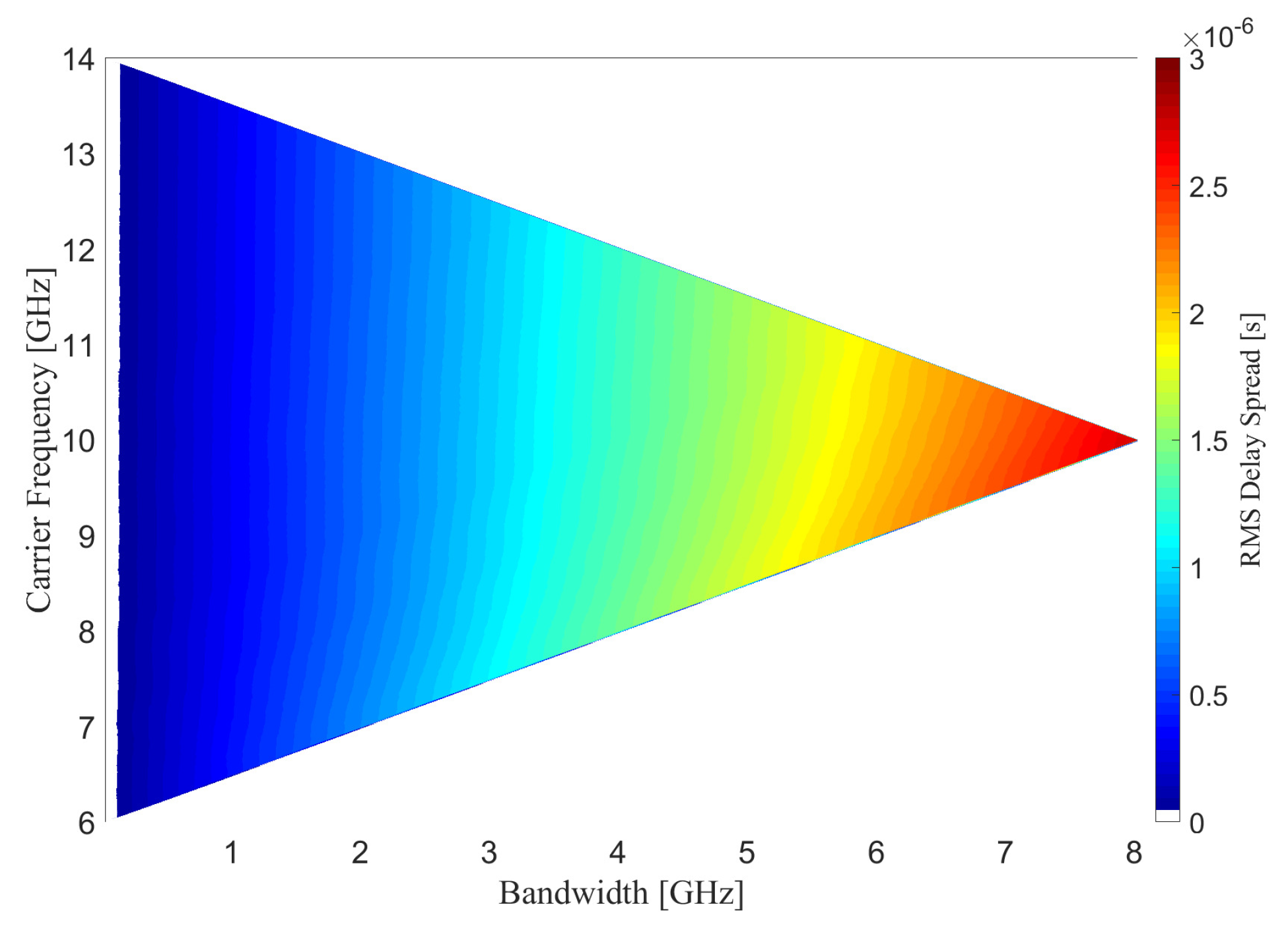
3.2.2. Frequency Selective Fading Analysis via RMS Delay Spread

It can be observed in Figure 9 that the RMS delay spread is negatively correlated with the carrier frequency, while positively correlated with the bandwidth. We infer that more MPCs appears in the channel with large bandwidth, resulting in the dispersion of power in delay. Thus, the delay dispersion effect is more evident, which leads to the increasing RMS delay spread. As for the decrease in RMS delay spread in carrier frequency domain, it is caused by the attenuation in high-frequency band according to the PL model.

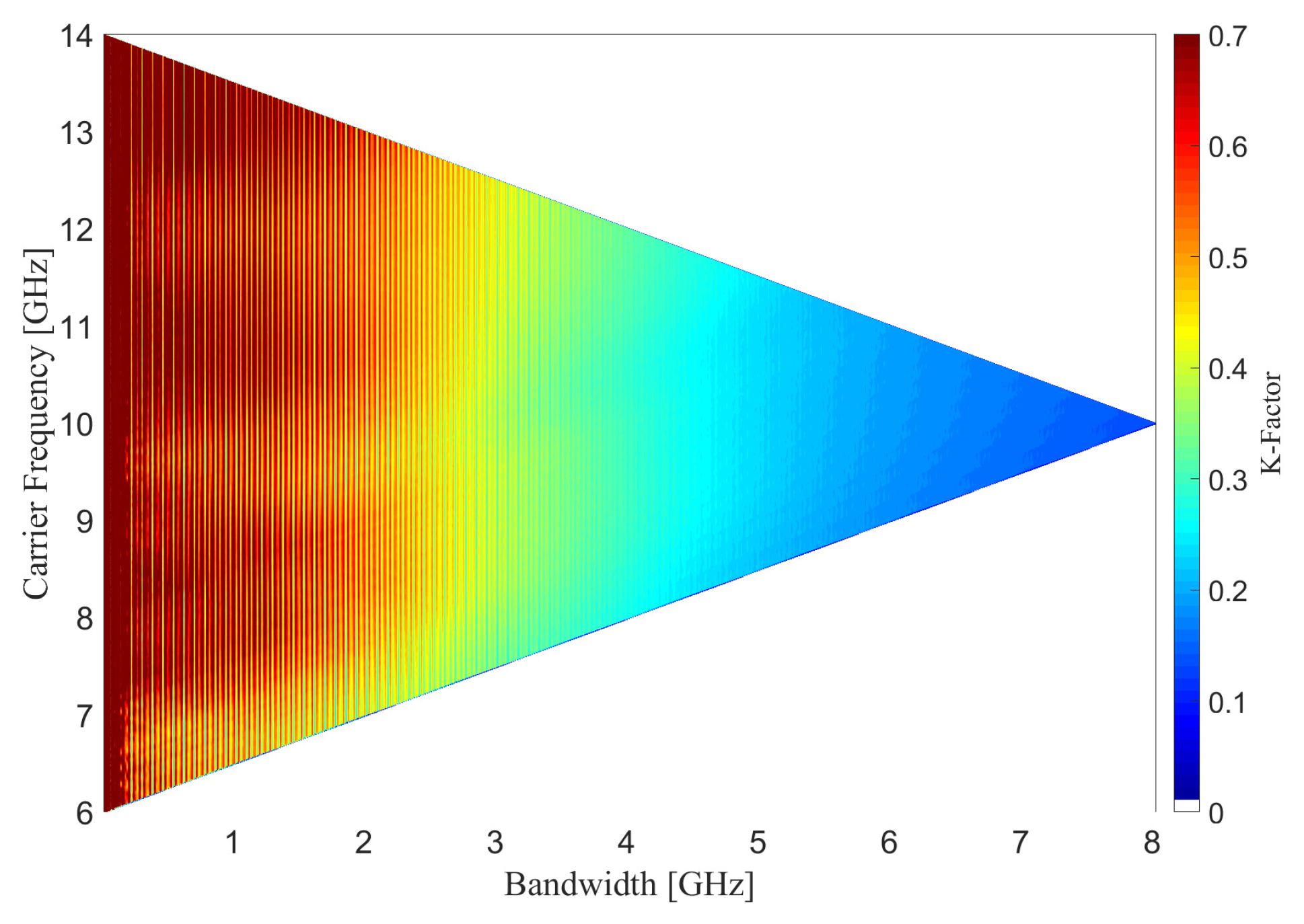
3.2.3. Channel Fading Characteristic Analysis via K-Factor

Since the measurement was conducted in a complex indoor scenario, most of the K-Factor are less than 1, especially for the channel with large bandwidth, indicating the rich MPCs existing in the environment. The great changes of K-Factor with regards to the bandwidth observed in Figure 10 indicates the poor transmitting quality of the channel with many NLoS paths resulted by large bandwidth. Moreover, in the channel with small bandwidth, K-Factor shows regular ups and downs in carrier frequency domain similar to the results in Figure 4, which is caused by the superposition of MPCs, as speculated.

3.3. Channel Characteristics Variation with regards to Antenna Elements

Sparsity analyses for wideband channels in the spatial domain have been verified by SDoF as summarized in [23], the metric of which depends on propagation conditions and antenna aperture sizes only. Similarly, in this indoor scenario, larger antenna aperture size causes larger SDoF and decreasing sparsity of the channel in space. Figure 3b illustrates the power distribution of one LoS path on the large antenna array. Further analyses focused on the dimension of antenna elements, which are extended to the RMS delay spread and K-Factor in this section.

3.3.1. Frequency Selective Fading Analysis via RMS Delay Spread

Figure 11 is the RMS delay spread in the receiving antenna array by rows and columns with changing carrier frequencies and fixed bandwidth, which describes the variation of received power in the spatial domain. The scales of the RMS delay spread shown in the figures below are fixed to compare the differences in values vertically and horizentally. The observations are concluded as follows:

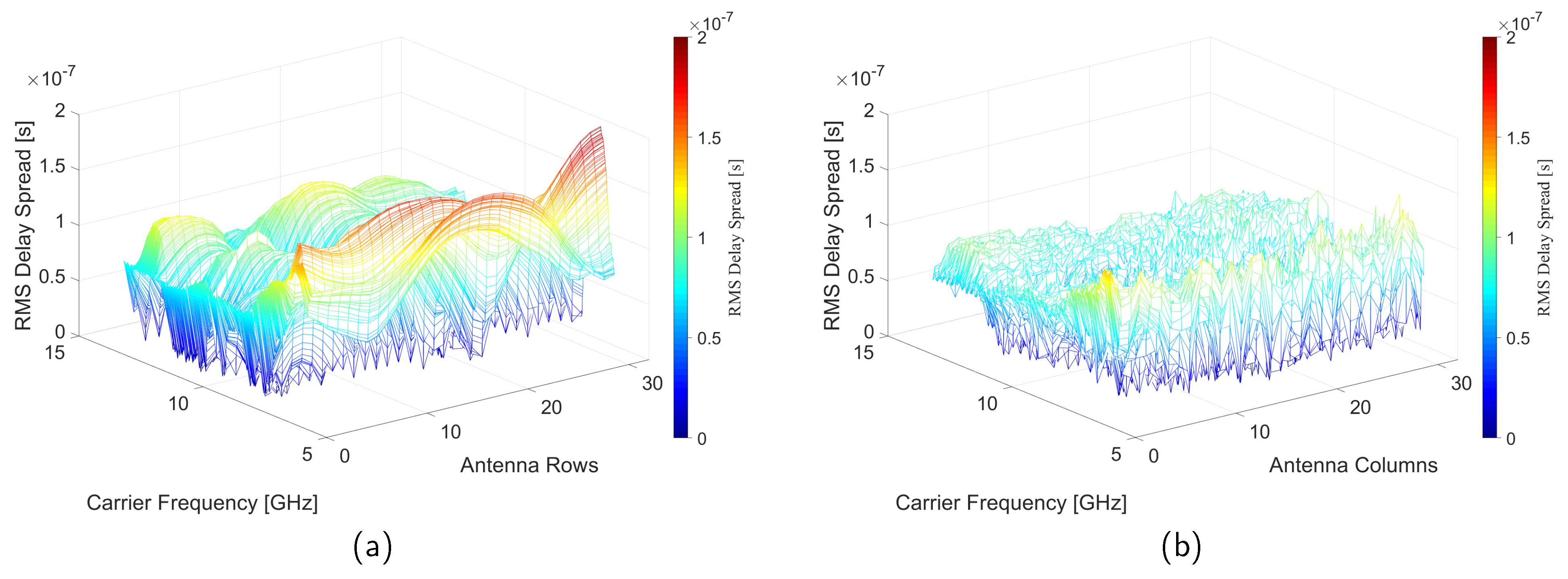
• In general, the changes of RMS delay spread are more significant in the perspective of carrier frequency than antenna elements. As explained above, the high carrier frequency causes high path loss and decreases RMS delay spread.
• With specified carrier frequency, the values of RMS delay spreads in antenna rows are larger than that in antenna columns. The interpretation can be derived accroding to the spatial power distribution in Figure 3b: the larger values in Figure 11a reflect the severe power changes in a row, while the smaller values in Figure 11b show the minor changes in a column.
• The variations of RMS delay spreads in antenna rows are more severe than that in antenna columns. This observation reveals the rich scattering effect in the environment, especially in terms of antanna rows. Mapping to the measurement environment, the scatterers are vertically stratified in the classroom with similar scatterer distributions at the same height. In different rows, the different scatterer distributions lead to different channel fadings, which is reflected in the severe variation of RMS delay spread, which is the opposite in different columns.
• For quantitative analysis, the total size of the virtual antenna array is around $33\times 33$ [cm${}^2$]. However, in such a small space, the RMS delay spread changes from $5\times {10}^{-8}$ [s] to $2\times {10}^{-7}$ [s] in a certain carrier frequency band. Thus, the environment has a great influence on the wideband channel.

3.3.2. Channel Fading Characteristic Analysis via K-Factor

• Opposite to RMS delay spread, the K-Factor is larger in higher frequency band. With great attenuation, the number and power of NLoS paths are decreased more critically compared to LoS paths. Therefore, the K-Factor increase with increasing carrier frequency.
• Figure 12b shows a trend that K-Factor increases greatly in large columns. The reason for this could be similar in Section 3.1.3 that the pilaster near Position 1 is on the left, which brings more MPCs in small columns, causing the dominance of NLoS paths.

3.4. Impact of User Locations on Channel Characteristics

Researches on propagation channel in MU scenarios have a great influence on channel sensing in 6G systems. In this paper, measurement was conducted in four different user locations. The results of different characteristics in different locations reflect spatial consistency with similar phenomena in the above dimensions, and also declare the differences of the channel in detail, quantitatively. In the wideband channel, the influences of user locations are summarized as follows.

• The similar distributions of the power are observed in Figure 3 with small lags in delay.
• The channel quality is illustrated in the carrier frequency domain in Figure 6 and Figure 7 in the form of RMS delay spread and K-Factor. The average values of K-Factor are increasing gradually in the four user locations, because of the scatterers’ distribution in the environment.
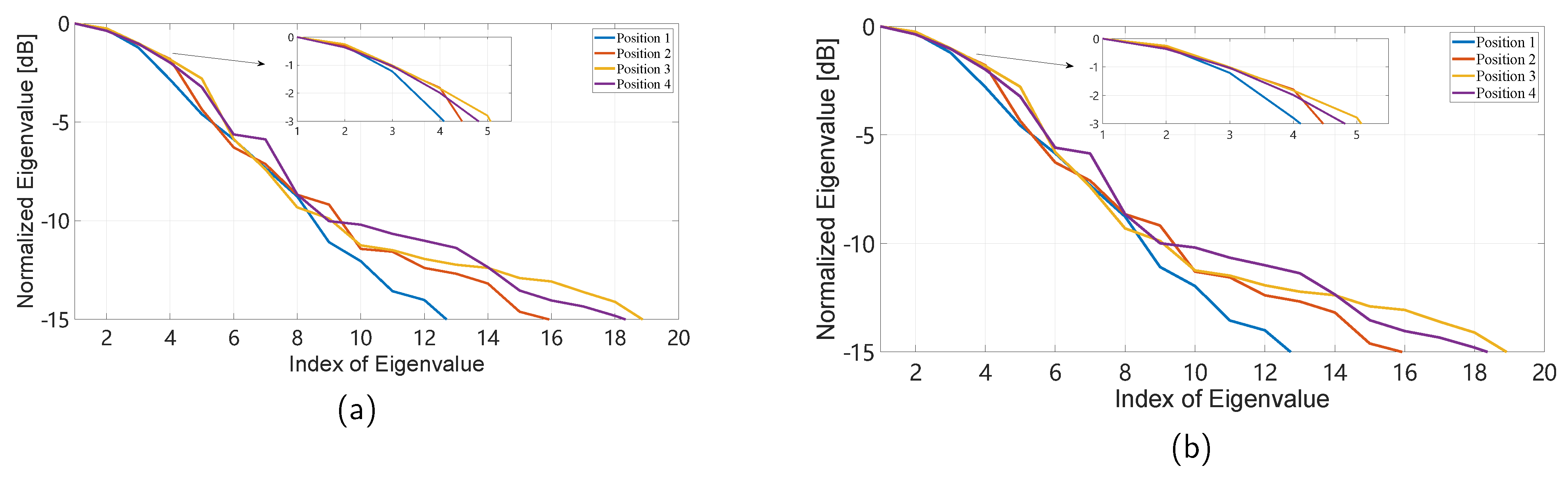
• The sparsity of the channel in frequency and spatial domains with different user locations is introduced in Figure 13. As location changes, the DoF in these two dimensions changes with a similar increasing trend in the long term, both showing that the channel is more sparse when closing to Position 1 with less MPCs.

4. Statistic Channel Models

4.1. Conventional Delay Spread Channel Model

cumulative distribution function (CDF) of the RMS delay spread in the indoor scenario is described in Figure 14 by Nakagami-Distribution, after comparing the root mean square error (RMSE) and R-Square tests. The data describes the RMS delay spread in all four user locations in the environment with the bandwidth varying from $0.8$ to 5 GHz, which indicates the channel behavior in the wideband channel in MU scenarios.

Theoretically speaking, the Nakagami distribution gives an approximate expression for the non-zero mean complex Gaussian distribution and is more realistic than Rayleigh, Rician and lognormal distributions, especially in the wideband channel. Results of the CDF model also indicate that Nakagami distribution is more consistent in wideband channel. The probability for the Nakagami distribution is shown in Equation (3), where ‘m’ is the shape factor reflecting the severity of the fading which should be more than 0.5, and $\Omega$ is the mean-square value of the distribution. The best fitting parameters for the RMS delay spread are $m=0.9000$ and $\Omega ={1.2111}^{-13}$ with all carrier frequencies, bandwidths and user locations.

$$P_{\mathrm{Nakagami}}\left(x\right)=\frac{2}{\mathsf{\Gamma }\left(m\right)}{\left(\frac{m}{\Omega }\right)}^m{x}^{2m-1}{e}^{-\frac{m}{\Omega }{x}^2}$$

(3)

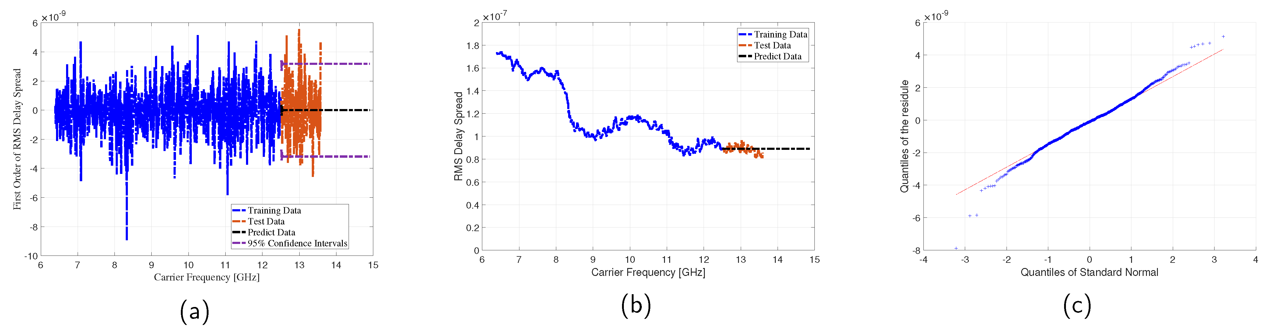
4.2. ARIMA Delay Spread Model

autoregressive integrated moving average model (ARIMA) model [26] is a widely used statistical method for time series prediction and is introduced to describe and predict the trend for RMS delay spread as shown in Figure 6.

Orders of the autoregressive (AR) and moving average (MA) process are chosen by Akaike information criterion (AIC) and Bayesian information criterion (BIC) principles, of which the value is the minimum. Moreover, the first-order difference is carried out to smooth the non-stationary RMS delay spread after the augmented dickey-fuller (ADF) test. Therefore, for the ARIMA ($p,d,q$) model, $p=2,d=1,q=2$.

The ARIMA model is fitted and evaluated by the training data and test data, which are separated from the first-order RMS delay spread, respectively.

Table 2. Fitting results for ARIMA model with a bandwidth of 8 GHz in an indoor scenario.

Parameter	Coefficient	p-Value
AR1	−1.1871	3.21 × 10${}^{-16}$
AR2	0.53607	2.16 × 10${}^{-5}$
MA1	1.1104	7.19 × 10${}^{-17}$
MA2	0.61568	5.23 × 10${}^{-10}$

shows the fitting results and p-value for the parameters. According to the statistical significance test method, p-value evaluates the probability of the sampling differences caused by the sampling error, which should be less than 0.05, as calculated below.

Notice that from the results shown in Figure 15a, long-term prediction results of the ARIMA method demonstrate the trend of the variation, rather than accurate values. The test data is mainly distributed between the lower and upper bounds of $95\%$ confidence intervals of the model, which fits the general range of the test data well. Figure 15b is the predicted RMS delay spread recovered from the first-order fitting, showing its trend.

Moreover, the evaluation of the model is conducted by the residue test and correlation test. quantile-quantile (Q-Q) plot is shown in Figure 15c, illustrating the correlation between the distributions of the residues and the standard normal. Theoretically, the distribution of the residues should satisfy the standard normal distribution as much as possible, which is verified above. As for the correlation test, the Durbin-Watson (D-W) test is conducted with the value of $2.0144$ close to two, indicating the irrelevance.

5. Conclusions

Wideband channel technology can be used to bring about more DoFs of the channel. In this paper, wideband channel behaviors including sparsity, frequency selective fading, and channel quality are introduced from the perspectives of carrier frequency, bandwidth, antenna elements and user locations at around 10 GHz. As shown in

Table 3. Summary of the characteristics.

	Carrier Frequency	Bandwidth	Antenna Elements	User Locations
DoF	Decreases monotonically	Increases monotonically	Influenced by antenna aperture size	Influenced by the neighboring environment
RMS delay spread	Decreases periodically	Increases monotonically	Changes severely vertically and horizontally
Rician K-Factor	Changes periodically	Decreases monotonically	Changes severely vertically and horizontally

, the consistency of the channel is observed in the first three dimensions, while the differences brought by the environment are reflected in different user loactions.

• In the carrier frequency domain, because of the severe path loss in high-frequency band, decreasing power leads to poor performance of the channel.
• Wide band brings more DoFs to the channel, increasing the rich scattering effects and influencing the time dispersion effect.
• From the perspective of different antenna elements, the wideband channel is stochastic with significant changes along the antenna rows, which is reflected in the environment. Moreover, in future work, research on channel performance in complicated environment with large antenna array needs to be considered, as it is influenced by the aperture of the large antenna array greatly in space.
• With different user locations, the characteristics are almost the same with slight differences because of the distribution of MPCs caused by the neighboring environment.

References

1. FCC. New Public Safety Applications and Broadband Internet Access Among Uses Envisioned by FCC Authorization of Ultra-Wideband Technology; Federal Communications Commission: Washington, DC, USA, 2002. [Google Scholar]
2. Yang, L.; Giannakis, G. Ultra-wideband communications: An idea whose time has come. IEEE Signal Process. Mag. 2004, 21, 26–54. [Google Scholar] [CrossRef]
3. Bas, C.U.; Ergen, S.C. Ultra-wideband Channel Model for Intra-vehicular Wireless Sensor Networks Beneath the Chassis: From Statistical Model to Simulations. IEEE Trans. Veh. Technol. 2013, 62, 14–25. [Google Scholar] [CrossRef] [Green Version]
4. Cassioli, D.; Win, M.; Molisch, A. The ultra-wide bandwidth indoor channel: From statistical model to simulations. IEEE J. Sel. Areas Commun. 2002, 20, 1247–1257. [Google Scholar] [CrossRef] [Green Version]
5. Molisch, A. Ultrawideband propagation channels-theory, measurement, and modeling. IEEE Trans. Veh. Technol. 2005, 54, 1528–1545. [Google Scholar] [CrossRef]
6. Keignart, J.; Daniele, N. Subnanosecond UWB channel sounding in frequency and temporal domain. In Proceedings of the 2002 IEEE Conference on Ultra Wideband Systems and Technologies (IEEE Cat. No.02EX580), Baltimore, MD, USA, 21–23 May 2002; pp. 25–30. [Google Scholar]
7. Ghassemzadeh, S.; Jana, R.; Rice, C.; Turin, W.; Tarokh, V. Measurement and modeling of an ultra-wide bandwidth indoor channel. IEEE Trans. Commun. 2004, 52, 1786–1796. [Google Scholar] [CrossRef]
8. Molisch, A.; Foerster, J.; Pendergrass, M. Channel models for ultrawideband personal area networks. IEEE Wirel. Commun. 2003, 10, 14–21. [Google Scholar] [CrossRef]
9. Venkatesh, S.; Ibrahim, J.; Mckinstry, D.R.; Buehrer, R.M. A spatio-temporal channel model for ultra-wideband indoor NLOS communications. IEEE Trans. Commun. 2009, 57, 3552–3555. [Google Scholar] [CrossRef]
10. Rappaport, T.S.; Xing, Y.; Kanhere, O.; Ju, S.; Madanayake, A.; Mandal, S.; Alkhateeb, A.; Trichopoulos, G.C. Wireless Communications and Applications Above 100 GHz: Opportunities and Challenges for 6G and Beyond. IEEE Access 2019, 7, 78729–78757. [Google Scholar] [CrossRef]
11. Abbasi, N.A.; Gomez-Ponce, J.; Shaikbepari, S.M.; Rao, S.; Kondaveti, R.; Abu-Surra, S.; Xu, G.; Zhang, C.; Molisch, A.F. Ultra-Wideband Double Directional Channel Measurements for THz Communications in Urban Environments. In Proceedings of the ICC 2021—IEEE International Conference on Communications, Montreal, QC, Canada, 14–23 June 2021; pp. 1–6. [Google Scholar] [CrossRef]
12. Maccartney, G.R.; Rappaport, T.S.; Sun, S.; Deng, S. Indoor Office Wideband Millimeter-Wave Propagation Measurements and Channel Models at 28 and 73 GHz for Ultra-Dense 5G Wireless Networks. IEEE Access 2015, 3, 2388–2424. [Google Scholar] [CrossRef]
13. Sangodoyin, S.; Molisch, A.F. A Measurement-Based Model of BMI Impact on UWB Multi-Antenna PAN and B2B Channels. IEEE Trans. Commun. 2018, 66, 6494–6510. [Google Scholar] [CrossRef]
14. Adeogun, R. On Propagation Graph Model for Industrial UWB Channels. In Proceedings of the 2021 IEEE International Symposium on Antennas and Propagation and USNC-URSI Radio Science Meeting (APS/URSI), Singapore, 4–10 December 2021; pp. 911–912. [Google Scholar] [CrossRef]
15. Qi, L.; Wang, L.; Gan, Z. Ultra Wideband Channel Estimation Based on Adaptive Bayesian Compressive Sensing with Weighted Eigen Dictionary. In Proceedings of the 2019 11th International Conference on Wireless Communications and Signal Processing (WCSP), Xi’an, China, 23–25 October 2019; pp. 1–4. [Google Scholar] [CrossRef]
16. WRC. Studies on Frequency-Related Matters for the Terrestrial Component of International Mobile Telecommunications Identification in the Frequency Bands 3300–3400 MHz, 3600–3800 MHz, 6425–7025 MHz, 7025–7125 MHz and 10.0–10.5 GHz. In Proceedings of the World Radiocommunication Conference 2019, Sharmel-Sheikh, Egypt, 28 October–22 November 2019; Available online: https://www.itu.int/md/R20-RAG-INF-0004/en (accessed on 1 September 2022).
17. WRC. Sharing and Compatibility Studies between Land-Mobile, Fixed and Passive Services in the Frequency Range 275–450 GHz. In Proceedings of the World Radiocommunication Conference 2019, Sharmel-Sheikh, Egypt, 28 October–22 November 2019; Available online: https://www.itu.int/pub/R-REP-SM.2450-2019 (accessed on 1 September 2022).
18. Yu, Y.; Rodríguez-Piñeiro, J.; Shunqin, X.; Tong, Y.; Zhang, J.; Yin, X. Measurement-Based Propagation Channel Modeling for Communication between a UAV and a USV. In Proceedings of the 2022 16th European Conference on Antennas and Propagation (EuCAP), Madrid, Spain, 27 March–1 April 2022; pp. 1–5. [Google Scholar] [CrossRef]
19. Wu, T.; Yin, X.; Zhang, L.; Ning, J. Measurement-Based Channel Characterization for 5G Downlink Based on Passive Sounding in Sub-6 GHz 5G Commercial Networks. IEEE Trans. Wirel. Commun. 2021, 20, 3225–3239. [Google Scholar] [CrossRef]
20. Zaman, K.; Mowla, M.M. A Millimeter Wave Channel Modeling with Spatial Consistency in 5G Systems. In Proceedings of the 2020 IEEE Region 10 Symposium (TENSYMP), Dhaka, Bangladesh, 5–7 June 2020; pp. 1584–1587. [Google Scholar] [CrossRef]
21. Zhao, X.; Du, F.; Geng, S.; Sun, N.; Zhang, Y.; Fu, Z.; Wang, G. Neural network and GBSM based time-varying and stochastic channel modeling for 5G millimeter wave communications. China Commun. 2019, 16, 80–90. [Google Scholar] [CrossRef]
22. Zhu, P.; Yin, X.; Rodríguez-Pineiro, J.; Chen, Z.; Wang, P.; Li, G. Measurement-Based Wideband Space-Time Channel Models for 77GHz Automotive Radar in Underground Parking Lots. IEEE Trans. Intell. Transp. Syst. 2022, 23, 19105–19120. [Google Scholar] [CrossRef]
23. Haneda, K.; Khatun, A.; Gustafson, C.; Wyne, S. Spatial Degrees-of-Freedom of 60 GHz Multiple-Antenna Channels. In Proceedings of the 2013 IEEE 77th Vehicular Technology Conference (VTC Spring), Dresden, Germany, 2–5 June 2013; pp. 1–5. [Google Scholar] [CrossRef]
24. Poon, A.; Brodersen, R.; Tse, D. Degrees of freedom in multiple-antenna channels: A signal space approach. IEEE Trans. Inf. Theory 2005, 51, 523–536. [Google Scholar] [CrossRef]
25. Yin, X.; Cheng, X. Propagation Channel Characterization, Parameter Estimation, and Modeling for Wireless Communications; John Wiley & Sons Singapore Pte. Ltd.: Singapore, 2018. [Google Scholar] [CrossRef]
26. Mills, T.C. Applied Time Series Analysis; Elsevier: Amsterdam, The Netherlands, 2019. [Google Scholar] [CrossRef]
Figure 1. Real and digital pictures of the measurement scenario. (a) The photo taken at the view of Rx. (b) The 3D digital map of the indoor scenario.
Electronics 11 03675 g001
Figure 2. Movement of the virtual antenna array.
Electronics 11 03675 g002
Figure 3. PDP of the channel observed in an indoor classroom scenario. (a) Power distribution in different delays at 4 locations. (b) Power distribution in spatial domain for one LoS path at Position 2.
Electronics 11 03675 g003
Figure 4. The variations of power with different delays and carrier frequencies at Position 2 and Position 4. (a) Power gain with different delays in frequency domain. (b) Power gain with different delays. (c) Power gain in frequency domain.
Electronics 11 03675 g004
Figure 5. The normalized eigenvalues versus eigenvalue index obtained for different carrier frequencies at Position 2.
Electronics 11 03675 g005
Figure 6. The RMS delay spread versus carrier frequency observed at 4 user locations.
Electronics 11 03675 g006
Figure 7. The K-Factor versus carrier frequency observed at 4 user locations.
Electronics 11 03675 g007
Figure 8. The normalized eigenvalues versus eigenvalue index obtained for different bandwidths at Position 2.
Electronics 11 03675 g008
Figure 9. The RMS delay spread versus carrier frequency and bandwidth at Position 2.
Electronics 11 03675 g009
Figure 10. The K-Factor versus carrier frequency and bandwidth at Position 2.
Electronics 11 03675 g010
Figure 11. The RMS delay spread versus carrier frequency and antenna elements at Position 2. (a) The RMS delay spread in different rows. (b) The RMS delay spread in different columns.
Electronics 11 03675 g011
Figure 12. The K-Factor versus carrier frequency and antenna elements at Position 2. (a) The K-Factor in different rows. (b) The K-Factor in different columns.
Electronics 11 03675 g012
Figure 13. The normalized eigenvalues versus eigenvalue index obtained in frequency and spatial domains at 4 user locations. (a) The normalized eigenvalues versus eigenvalue index in frequency domain. (b) The normalized eigenvalues versus eigenvalue index in spatial domain.
Electronics 11 03675 g013
Figure 14. The CDF of RMS delay spread.
Electronics 11 03675 g014
Figure 15. ARIMA fitting and evaluating for RMS delay spread with fixed bandwidth. (a) ARIMA fitting for first-order RMS delay spread. (b) Fitting results for RMS delay spread. (c) Residual analysis.
Electronics 11 03675 g015