Article

Mixed Electric Field of Multi-Shaft Ship Based on Oxygen Mass Transfer Process under Turbulent Conditions

College of Electrical Engineering, Naval University of Engineering, Wuhan 430033, China
*
Author to whom correspondence should be addressed.
Electronics 2022, 11(22), 3684; https://doi.org/10.3390/electronics11223684
Submission received: 9 September 2022 / Revised: 8 October 2022 / Accepted: 4 November 2022 / Published: 10 November 2022
(This article belongs to the Section Circuit and Signal Processing)

Abstract

:
The theoretical basis for a multi-physics coupling modeling involving a turbulence flow field and a ship’s electric field was analyzed using the principles of electrochemistry and hydrodynamics. Considering the mass transfer of oxygen in the cathode reaction of electrochemical corrosion, the boundary element method was adopted to construct a corrosion electric field model for a multi-shaft ship under navigation. After dissecting the equivalent circuit resistance of the mechanical structure of a ship’s shaft, the initial phase difference of the equivalent resistance between different shafting systems of a multi-shaft ship was analyzed to reveal the regularity of variation of the ship corrosion mixed electric field, when the contact positions of the shaft grounding device were different. A ship model experiment was conducted to verify the correctness of the simulation model. As shown in the results, when the initial phase difference of two-shaft ship shafting equivalent resistance increased from 0° to 45°, 90°, 135°, and 180°, the amplitude of the ship’s mixed electric field varied by less than 3.7%, which was practically negligible. However, the amplitude of the ship’s shaft-rate electric field decreased by 8.30%, 25.4%, 50.2%, and 88.0%, respectively. Moreover, the minimum value of the shaft-rate electric field accounted for 4.11% of the maximum value. This significantly increased the difficulty of marine target detection based on electric field sensors.

1. Introduction

At present, the detection of marine targets mostly uses the sound field as the characteristic signal. With the research on the magnetic field and electric field of ships, the multi-sensor fusion detection and positioning technology for simultaneously detecting the magnetic field, electric field, and sound field has been gradually applied. Among them, the ship’s electric field signal, especially the shaft-rate electric field signal, is distinctive in the ocean, and transmits over long distances, so that it has been widely applied in the remote detection of marine targets [1]. Therefore, it is of great significance to study the variation regularity of the ship’s electric field under sailing conditions.
A hull made of different metals is connected by a shafting mechanical structure to the propeller, which generates galvanic corrosion in seawater [2]. When the ship is sailing, the corrosion loop has the current modulated by the rotation of the shafting mechanical structure, which creates a mixed electric field around the ship. The mixed electric field consists of an electrostatic field and a shaft-rate electric field. With the demand for increasing velocity, multi-shaft and multi-propeller ships have been extensively applied. A multi-shaft ship contains a complex shafting mechanical structure. The corrosion current varies with the fluctuation of the resistance of its corrosion loop equivalent circuit, which eventually affects the phase, amplitude, frequency, and other characteristics of the ship’s mixed electric field.
Current studies of the electric fields of ships have focused on cathode protection for ships [3], which has been successfully achieved and maintained for a long period of time by optimizing the position of an assisted anode [4,5]. Many studies have been carried out on the electrochemical characteristics of metals and anti-corrosion methods in flowing seawater [6,7]. The research also focuses on the electrochemical characteristics of metal corrosion and cathodic protection methods under deep-sea high-pressure environments [8,9]. At the same time, in research on underwater target positioning through the electric field [10], the inversion of coating damage location by the underwater electric field has also been extensively studied [11,12]. The research of the ship corrosion electric field is of great significance [13]. At present, electric dipole is a mature model for studying the electric field [14]. This type of modeling provides a well-developed, simple, and effective method for simulating this type of electric field. However, multiple physical fields such as flow fields, electric fields, and the mass transfer process must be coupled to accurately simulate the mixed electric field of a ship during navigation.
In this paper, the regularity in variation of equivalent resistance of a ship shafting mechanical structure is analyzed, and the three-dimensional modeling software is used to carry out the three-dimensional modeling of the multi-shaft ship. Moreover, multi-physics coupling simulation is performed using multi-physics simulation software, and the boundary element method is adopted to calculate a ship’s electric field [15,16] to analyze the regularity in variation of the electric field of a multi-shafted ship. This method is of great significance to the study of the variation law of the electric field of multi-shafted ships under sailing conditions.

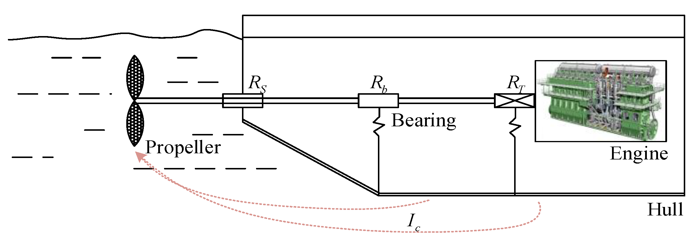
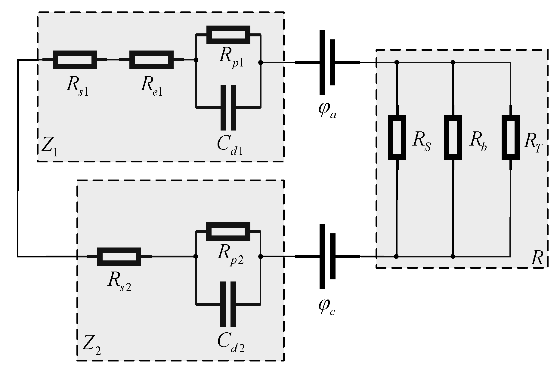
2. Equivalent Model of Shafting Mechanical Structure

The ship corrosion electric field consists of an electrostatic field and a shaft-rate electric field. For a ship under navigation, the corrosion current is modulated by the propeller and the mechanical structure of the shaft. The generation mechanism of the shaft-rate electric field is that the corrosion current passes through the internal loop of the hull of the “propeller–spindle–main shaft grounding–hull” [17] (Figure 1). Modeling of the shaft-rate electric field entails an analysis of the equivalent circuit for such an internal loop.
Figure 2 shows that the equivalent circuit of the ship corrosion loop has resistance defined by:
Z = Z 1 + Z 2 + R
where Z 1 contains the leakage resistance of the hull surface in the seawater medium R s 1 , the impedance of the hull surface coating (including the coating resistance R e 1 and coating capacitive reactance 1 / ω C c 1 ), and the polarization impedance of the hull surface (including the polarization resistance R p 1 and the electric double-layer capacitive reactance of surface 1 / ω C d 1 ). Z 2 contains the leakage resistance of the propeller surface R s 2 in seawater, and the polarization impedance of the propeller surface (including the polarization resistance R p 2 and the electric double-layer capacitive reactance of surface 1 / ω C d 2 ). When a ship is sailing, the periodic variation of the electric double-layer capacitive reactance of the hull and propeller surface, C d 1 and C d 2 , causes a change in the resistance, Z 1 and Z 2 , respectively, which is known as external modulation of the corrosion electric field. The capacitive reactance of Z 1 and Z 2 is calculated as follows:
Im Z 1 = ω C d 1 R p 1 2 1 + ω 2 C d 1 2 R p 1 2
Im Z 2 = ω C d 2 R p 2 2 1 + ω 2 C d 2 2 R p 2 2
where C d 1 = b 1 ω β 1 S 1 , C d 2 = b 2 ω β 2 S 2 , R p 1 = a 1 ω α 1 S 1 , R p 2 = a 2 ω α 2 S 2 , and ω = 2 π f .
In the calculation, a ship has a submerged hull area, S 1 = 4000   m 2 , and a two-shaft propeller surface area, S 2 = 60   m 2 . The hull and propeller are made of steel and copper alloys, respectively. Based on their chemical characteristics of alternating current, the a , b , α , and β values of the submerged hull area and two-shaft propeller surface are 40, 2.7, −0.64, and −0.22, as well as 0.177, 2.45, −0.31, and −0.46, respectively. When the rotational speed of the propeller is 2 r / s , only the influence of the external modulation of electric field corrosion is considered, so that there is: Δ | C d | = Im Z 1.7   m Ω .
In Equation (1), R contains the sealed bearing resistance R S , shaft grounding resistance R b , and thrust bearing resistance R T . The bearing resistance exists inside the hull where no seawater enters, so that it is also known as the internal modulation of the corrosion electric field. The shaft grounding device is mainly composed of a carbon brush and a slip ring, and its contact resistance R b is much lower than the bearing resistances R S and R T . The internal modulation resistance is connected in parallel, so that it is set as R R b . The shaft grounding device composed of a copper graphite carbon brush and a copper-based slip ring has the resistance R b equivalent to 20   m Ω , and its resistance fluctuation coefficient is around 10–30%; that is, Δ R b 2 ~ 6   m Ω . Considering the slight fluctuation of basic seawater parameters such as temperature and oxygen concentration, the variation of the electric double-layer capacitive reactance on the ship surface, Δ | C d | , is much lower than the variation of shaft grounding resistance, Δ | R b | . The frequency of the ship’s electric field is primarily caused by internal modulation. Hence, the equivalent resistance of the ship shafting mechanical structure can be set to:
R = 20 + 5 sin ( 2 π f t + φ ) ( m Ω )
where f is the shafting rotation frequency, and φ is the initial phase of the shafting equivalent resistance, that is, the angle formed by the initial contact position of the shaft grounding bearing carbon brush and slip ring.

3. Ship’s Electric Field Model

For a ship under navigation, the increasing velocity and rotational speed of the propellers causes a higher flow rate of a corrosive medium and a higher rate of oxygen transfer to the surface of the propeller blade. At the position of a higher flow rate, more oxygen molecules are involved in the galvanic corrosion reduction reaction, which increases the density of the corrosion current and further affects the distribution of the corrosive electric field of the ship. For this reason, a multi-physics coupling model must be constructed for the corrosion electric field of a multi-shaft ship under navigation, to analyze the regularity of variation of the mixed electric field. This model contains a flow field, an electric field, and the mass transfer process.

3.1. Turbulence Physics Modeling

For a ship under navigation, the rotation Reynolds number of a propeller is approximately 107, so that a turbulence physics model must be adopted.
R e = n D 2 μ
where n is the rotational speed of the propeller, D is the diameter of the propeller, and μ is the kinematic viscosity factor.
Turbulence is a state of the flow field where the rotation of the propeller increases the velocity of the water and creates eddies. Presently, the Reynolds Average Navier–Stokes (RANS) equation is often used for the numerical simulation of fluids. In the equation, the turbulence flow rate, u , is broken down into an average, u , and a fluctuating part, u . Based on the Boussinesq assumption, it is transformed into the problem of solving the turbulence viscosity, μ T . In this paper, the standard k ε model is employed for calculation, while the turbulence kinetic energy, k , and the turbulence dissipation rate, ε , are introduced to represent the turbulence viscosity, μ T . Moreover, two transmission equations are added as follows [18]:
μ T = ρ C μ k 2 ε
ρ k t + ρ u k = [ ( μ + μ T σ k ) k ] + p k ρ ε
ρ ε t + ρ u ε = [ ( μ + μ T σ ε ) ε ] + C ε 1 ε k P k C ε 2 ρ ε 2 k
The term p k is generated as:
p k = μ T ( u : ( u + ( u ) T ) 2 3 ( u ) 2 2 3 ρ k u
where ρ is the density of an incompressible fluid. In Equations (6) to (9), the constants including C μ , C ε 1 , C ε 2 , σ k , and σ ε were measured during the experiment as 0.09, 1.44, 1.92, 1.0, and 1.3, respectively.

3.2. Modeling for Mass Transfer of Oxygen

The mass transfer process of oxygen in seawater determines the strength of metal corrosion. Meanwhile, the distribution of the concentration of oxygen is subjected to the flow rate distribution of the fluid, so that the flow rate variables must be coupled for calculation. It is assumed that the anode and cathode of galvanic corrosion are made of 921 A steel and B10 copper alloy [19], which experience oxidation and reduction reaction [20], respectively, in the hull and propeller. For example:
F e F e 2 + + 2 e O 2 + 2 H 2 O + 4 e 4 O H
In the steady mass transfer process, the mass-conservation equation for the transfer of a simulated chemical substance in the convection and diffusion transfer mechanism is:
( D c ) + u c = R
where D is the diffusion coefficient of the substance, c is the concentration of the substance, and c is the oxygen concentration, since this paper focuses on how an electric field is affected by the mass transfer of oxygen. The surface flow rate, u , can be obtained using the above RANS equation. In the equation, R is the reaction rate of the substance, and is represented by:
R = v i l o c n F
where i l o c is the local current density of the chemical reaction, which can be obtained by the surface electrode kinetic equation for the galvanic corrosion electrode, v is the number of electrons in the chemical reaction, which is 4 for the cathode oxygen absorption corrosion in the galvanic corrosion, and F is the Faraday constant.

3.3. Modeling for a Ship’s Electric Field with the Boundary Element Method

In this paper, the boundary element method is used in the three-dimensional modeling for a ship’s electric field. In the turbulence physics field at the cathode propeller, the oxygen concentration and corrosion electrochemical reaction will affect each other. The electrode kinetic equation adopts the concentration-dependent Butler–Volmer equation as follows:
i l o c = i 0 ( ( C R C R , r e f exp ( α a F η R T ) C o C o , r e f exp ( α c F η R T ) )
where i 0 is the exchange current density, which is 7.7 × 10⁻⁷  A / m 2 in the copper alloy surface oxygen reduction in the simulation, α a and α c are the anode and cathode transfer coefficients, respectively, R is the gas constant, F is the Faraday constant, η is the activation over-potential, which is the difference between the electrode potential and the equilibrium potentials, E e q , and the equilibrium potential of cathode oxygen is 0.189 V; meanwhile, c R , c o , and c R , r e f , c o , r e f are the reductant and the oxidant concentrations, and their initial references, respectively. The propeller surface oxygen concentration, c o , is obtained using Equation (11).
After calculating the electrode surface potential and local current density distribution with the electrode kinetic equation, the potential, φ i , at any field point i in the domain is solved with the boundary integral equation:
φ ( i ) + S φ ( ξ ) φ * ( i , ξ ) n ( ξ ) d S = S J ( ξ ) φ * ( i , ξ ) d S
The boundary element method is employed to discretize the boundary integral equation, so that the boundary S is discretized into N units. The boundary integral equation is expressed as:
φ i + j = 1 N φ i S j φ * n d S j = j = 1 N J j S j φ * d S j
where φ * = 1 4 π σ r , r is the distance from the field point i to the point ξ on the boundary surface, and σ is the seawater conductivity.
After obtaining the potential current by solving the matrix equation, the underwater electric field component and its modulus is calculated by:
{ E x = - φ x E y = - φ y E z = - φ z

4. Simulation Analysis

The ship’s electric field model based on multi-physics coupling modeling is combined with the analysis of the equivalent resistance of the ship shaft mechanical structure. With three-dimensional (3D) graphics software SOLIDWORKS 2016, a 3D geometric model was drafted for the underwater portion of the ship, and input into the simulation software COMSOL Multiphysics 5.4 for the simulation analysis of multi-physics coupling.
A seawater area with the conductivity of 4 S / m was set within a certain scope of the ship’s underwater portion (Figure 3). The vessel model used was 168 m in length, 20 m in width, and 8.6 m in depth. The sea domain used was 500 m in length, 100 m in width, and 50 m in depth. The propeller diameter was 4 m. The hull and rudders are made of 921 A steel, while the propeller consists of B10 bronze alloy. The vessel underwater surface and seawater domain were meshed, and mesh subdivision results are shown in the Figure 4, including 612,248 domain elements, 57,490 boundary elements, and 7329 edge elements. In the area, seawater flowed at the rate of 4 m / s from the bow to the stern of the ship. The corresponding rotational speed of the propeller was 2 r / s . A ship under navigation was simulated in this situation. For the simulation, the concentration-dependent Butler–Volmer equation was selected as the propeller surface polarization equation. The surface resistance was set to R = 20 + 5 sin ( 2 π f t + φ ) ( m Ω ) , and the rotational speed of both shafts was f = 2 Hz . The initial phase for the variation in resistance of the two shafting systems was set to φ 1   = 0 and φ 2   = 0 , 45 , 90 , 135 , 180 . Then, we analyzed how different initial phase differences, Δ φ , affect the ship’s mixed electric field, particularly, the shaft-rate electric field.

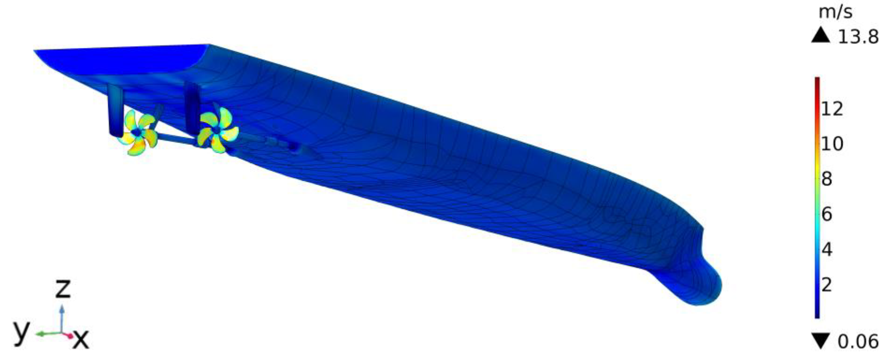
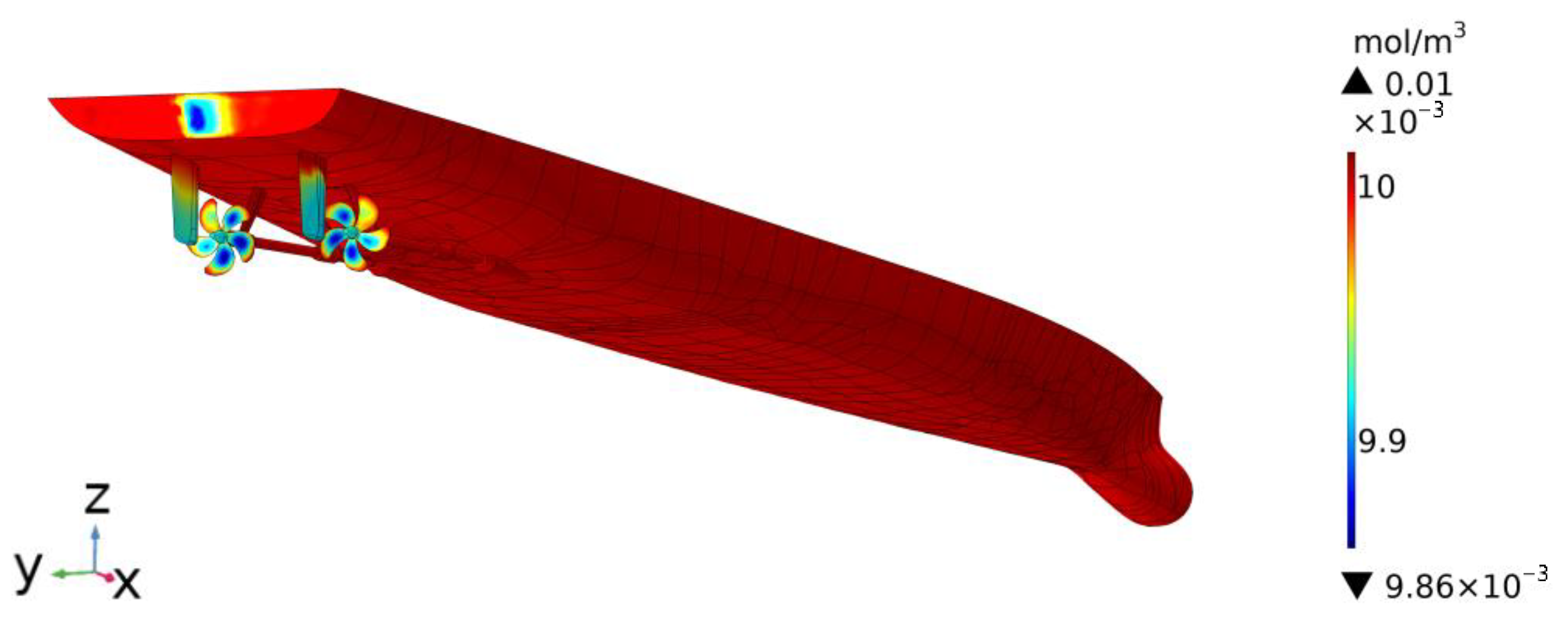
4.1. Ship Surface Flow Rate and Oxygen Concentration Distribution

When the ship has the velocity of 4 m / s and the propeller has a rotational speed of 2 r / s , the maximum flow rate at the underwater surface of the ship is 13.8 m / s , and the flow rate at the hull surface is close to the ship’s velocity, but significantly lower than the flow rate at the propeller surface (Figure 4). Figure 5 presents the ship underwater distribution of the surface oxygen concentration at the corresponding flow rates. It is observed that the distribution of the oxygen concentration on the propeller surface resembles the surface flow rate distribution. Affected by the mass transfer of oxygen molecules, more oxygen molecules are involved in the cathode reduction reaction of galvanic corrosion at a position with a higher flow rate, resulting in a lower oxygen concentration on the surface. Based on the electrode kinetic equation, that is, the concentration-dependent Butler–Volmer equation, local current density is greater when the ratio of the propeller surface oxygen concentration and its reference c o / c o , r e f is smaller. In the end, this leads to a higher intensity of the ship corrosion electric field compared with the stationary state. The ship underwater current density vector distribution and electric field distribution are shown in Figure 6 and Figure 7.

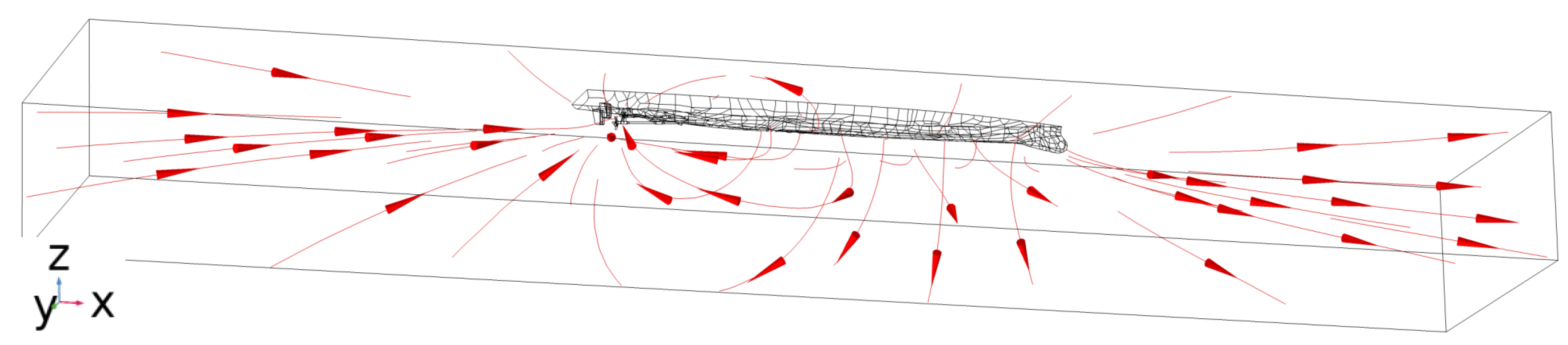
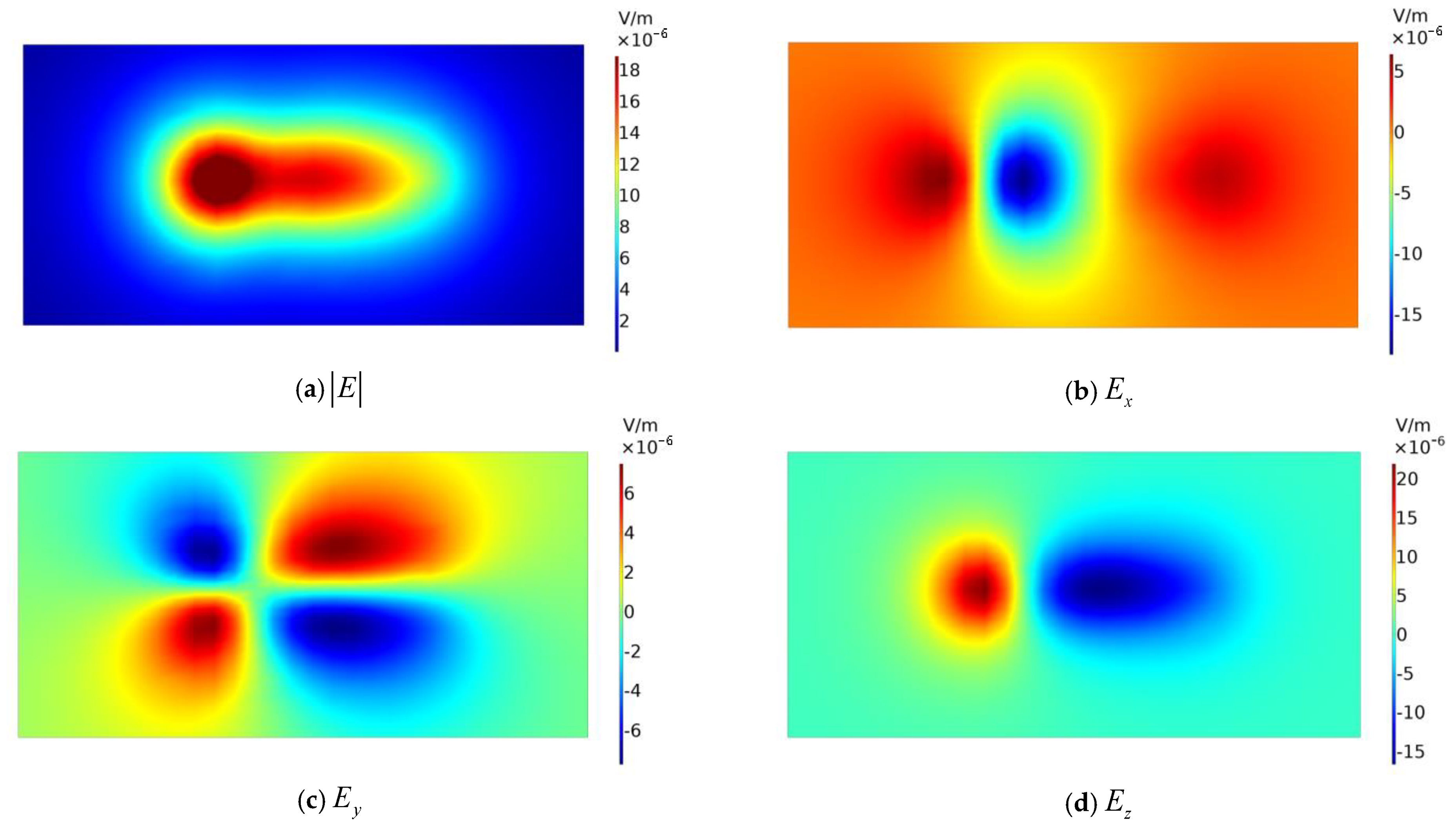
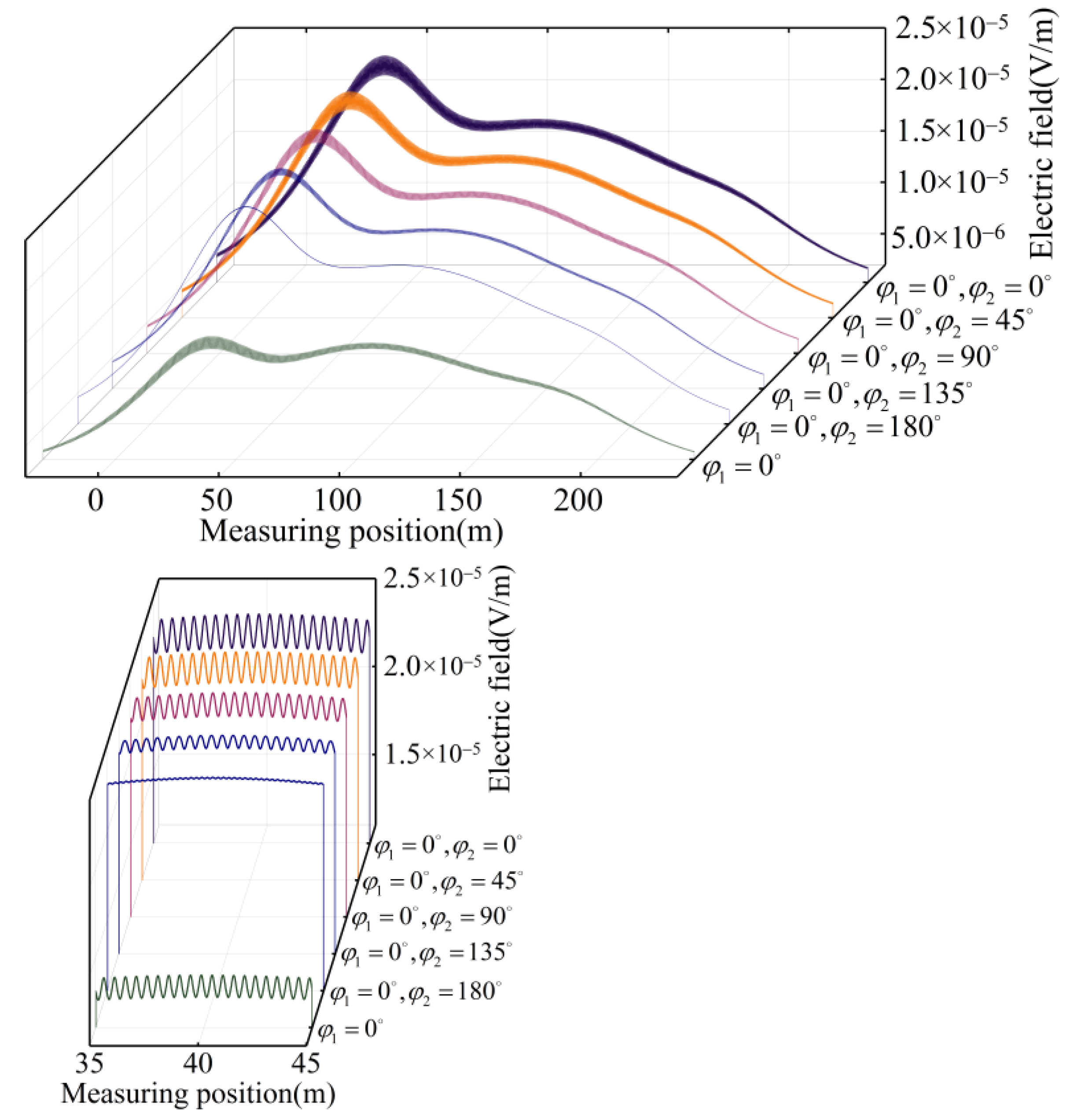
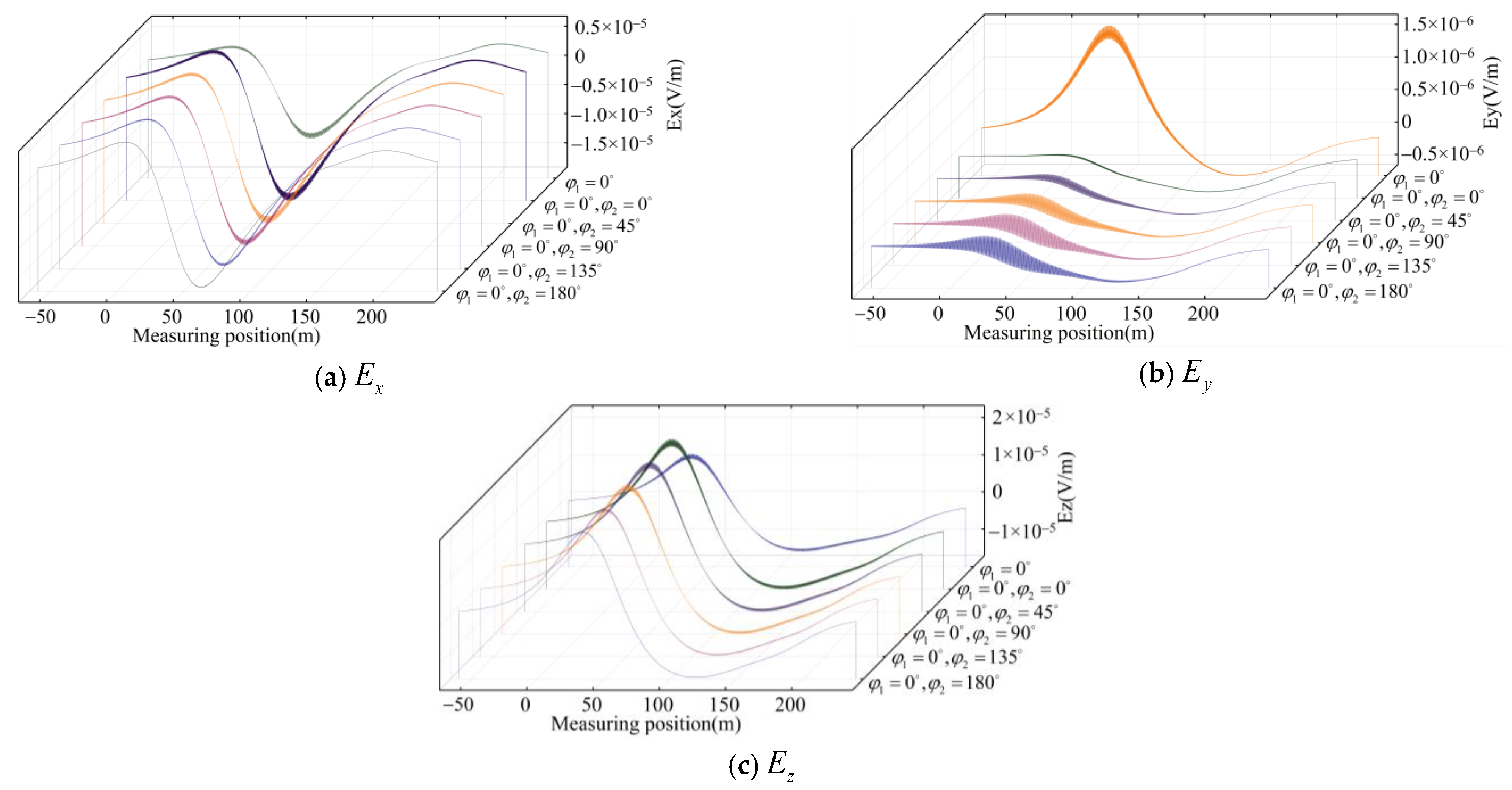
4.2. Ship’s Electric Field Distribution

With the horizontal measuring line set at twice the width of the ship underwater, the measuring point moved at the speed of 1 m / s from the stern to the bow to measure the distribution of the ship’s electric field for a while. The initial phase, φ 1 , of a two-shaft ship’s shifting equivalent resistance, R , was set to be 0° and φ 2 being 0°, 45°, 90°, 135°, or 180° to measure the ship’s mixed electric field. This was compared with a single-shaft ship of the same type. The ship’s mixed electric field is obtained by the superposition of the electrostatic field and the shaft-rate electric field (Figure 8) and fluctuated with the same frequency as the rotation of the propeller. The electric field amplitude occurs at x = 40   m , that is, right under the propeller. The mixed electric field amplitude is presented in Table 1. Evidently, the amplitude of the electric field of a two-shaft ship is around 1.7 times as large as that of the single-shaft ship when they have the same type of hull. Meanwhile, the variation of the initial phase difference, φ , of the two-shaft ship shafting equivalent resistance, R , exerts very little effect on the amplitude of the electric field.
After amplifying the electric field distribution curve at x = 40   m , we can clearly observe the maximum fluctuation of the ship’s electric field when the initial phase of the two-shaft ship’s shafting equivalent resistance is φ 1   = 0 and where φ 2   = 0 . However, the fluctuation gradually diminishes with the increase of the initial value of φ 2 until φ 2   = 180 . After low-pass filtering of the mixed electric field, the ship’s electrostatic field is obtained, but varies very slightly. Thus, the variation in the amplitude of the mixed electric field is mainly attributed to the shaft-rate electric field. The distribution of the XYZ component of the ship’s mixed electric field is shown in Figure 9. In terms of magnitude, the Z component is the main part of the mixed electric field. The two-shaft ship’s electric field counteracts in the Y direction, which is significantly lower than the single-shift ship’s mixed electric field.
The shaft-rate electric field is obtained after the band-pass filtering of the ship’s mixed electric field, as shown in Figure 10. The shaft-rate electric field is spindle-shaped, and its amplitude is associated with the initial phase of shafting resistance (Table 2). The shaft-rate electric field takes up around 4% of the ship’s mixed electric field. With the same type of hull, the amplitude of the shaft-rate electric field of a two-shafted ship is 1.5 times as great as that of a single-shafted ship. When the shafting equivalent resistance has no initial phase difference, Δ φ , the shaft-rate electric field reaches the maximum value of 9.812 × 10 7   V / m . With each increase of 45° in the initial phase difference, Δ φ , the shaft-rate electric field decreased by 8.30%, 25.4%, 50.2%, and 88.0%, respectively. When Δ φ   = 180 , the shaft-rate electric field gradually diminishes to the minimum value, accounting for only 4.11% in the case of no initial phase difference. After observing the x, y, and z components of the shaft-rate electric field (Figure 11), it was found that the z component of the electric field has a larger amplitude, and the x and z components vary in a similar way to the modulus variation of the shaft-rate electric field. Nevertheless, the y component of the electric field varies in an opposite way. It gradually increases with the increase of the initial phase difference, Δ φ , of the shafting equivalent resistance but exerts little effect on the modulus variation regularity of the shaft-rate electric field because of its low amplitude. The above results show that the shaft-rate electric field of the multi-shaft ship is offset in the y direction, and the offset effect is more obvious with the increase of the equivalent resistance initial phase difference, Δ φ . As the electric field line of the ship mainly points from the hull to the propeller, the amplitude of the electric field in the z direction is the largest. The variation rule of the y component of the shaft-rate electric field is opposite, because when the propeller of a two-shaft ship is completely axisymmetric, and Δ φ = 0 , Ey should be close to 0.
As shown in the results, the ship corrosion mixed electric field is modulated by the ship shafting mechanical structure, so that it varies periodically. A multi-shafted ship has a greater amplitude of the mixed electric field and shaft-rate electric field than a single-shafted ship. When different initial phases, φ , exist for the equivalent resistance of a two-shafted ship’s shafting mechanical structure, the amplitude of the ship’s mixed electric field varies within 3.7%, which is basically ignorable. However, the ship shaft-rate electric field obtained after filtering varies dramatically (Figure 12). When the initial phase difference of equivalent resistance is Δ φ   = 180 , the shaft-rate electric field takes up only 4.11% of the value at Δ φ   = 0 . The ship shaft-rate electric field has the amplitude up to the μ V / m scale, while the low-frequency spectrum in the frequency domain has the rotation of the main shaft as its fundamental frequency. The signal is highly distinctive in the ocean, and can be transmitted for long distances, so that it is widely applied in the remote detection of marine targets. With different initial phases, φ , of ship shafting equivalent resistance, a multi-shafted ship experiences a dramatic amplitude fluctuation of the ship shaft-rate electric field, which significantly increases the difficulty of marine target detection based on electric field sensors.

5. Experiment

To verify the correctness of the simulation results with the multi-physics coupling model built for the electric field of a multi-shaft ship, a scale model experiment was carried out in a laboratory environment. In the experiment, an underwater vessel was used with its hull surface covered by an evenly corroded steel coating, and with a single-shafted propeller made of nickel-aluminum-bronze. The hull and propeller materials were the same as the actual vessel, to reduce the error caused by the hull material itself. The size of the ship model was 1.2 m in length and 0.15 m in width. The propeller had its main shaft connected to the hull by virtue of a grounding carbon brush and rotated at the rate of 2 r / s under motor control. The experimental tank was 100 cm deep, and the seawater conductivity was 3.8 S / m . Three pairs of orthogonal Ag/AgCl sensors were located at twice of the ship breadth (30 cm) right under the vessel. The sampling frequency of sensors was 2.5 Khz. The passing curve for the ship corrosive electric field was measured.
The measured ship model’s electric field signal and its x, y, and z components were band-pass-filtered at 0.3–30 Hz to obtain the shaft-rate electric field modulus and its component signatures (Figure 13 and Figure 14), which was consistent with the simulation results. The ship shaft-rate electric field spectrum obtained by fast Fourier transform is shown in Figure 15. Obviously, the shaft-rate electric field takes the rotation frequency of the main shaft as its fundamental frequency, and its amplitude reached the μ V / m scale. It is therefore proven that the proposed multi-physics coupling model of a flow field and electric field based on the mass transfer of oxygen is basically correct. Due to the complex shafting mechanical structure of a multi-shafted ship, it is difficult to identify the coupling state of a shaft grounding device. Moreover, it is not easy to control where the shaft grounding bearing carbon brush contacts the slip ring, also causing possible contact at several positions. For this reason, the initial value, φ , of the equivalent resistance, R , for different shafting systems is uncertain in the simulation analysis, making it difficult to verify the simulation results; particularly, dramatic variation occurs in the ship shaft-rate electric field amplitude, through a ship model or in a real ship experiment.

6. Conclusions

In this paper, the theoretical basis of multiple physical field coupling modeling, such as the turbulent flow field and the ship’s electric field, was analyzed. Combined with the mass transfer process of the cathode reaction substance oxygen in the ship corrosion electrochemical reaction, a multi-shaft ship corrosion electric field model under navigation was established by using the boundary element method by analyzing the generation mechanism of the ship’s shaft-rate electric field; that is, the variation law of the equivalent resistance of the shafting mechanical structure in the modulation loop of the corrosion electric field. The influence of different equivalent resistance, R , and initial phase, φ , on the ship’s mixed electric field and shaft-rate electric field was analyzed. The following conclusions were drawn.
(1) As shown in the results, when the initial phase difference, Δ φ , of a two-shaft ship’s shafting equivalent resistance, R , increased from 0° to 45°, 90°, 135°, and 180°, the amplitude of a ship’s mixed electric field varied by less than 3.7%, which was practically negligible. However, the amplitude of the ship’s shaft-rate electric field decreased by 8.30%, 25.4%, 50.2%, and 88.0%, respectively. When the initial phase difference was Δ φ   = 180 , the shaft-rate electric field accounted for only 4.11% of the value at Δ φ   = 0 . Since the ship’s shaft-rate electric field is widely applied in the remote detection of marine targets, dramatic variation occurs in the ship’s shaft-rate electric field amplitude, which significantly increased the difficulty of marine target detection.
(2) Through the ship scale model experiment, the generated shaft-rate electric field was measured and compared with the simulation results, which verified the correctness of the established multi-shaft ship corrosion electric field model based on the mass transfer process of oxygen under turbulence.

Author Contributions

Writing—original draft preparation, S.W.; planning and performing the experiments, X.W.; theory consultation and formal analysis, X.W. and Y.H.; writing—review and editing, S.W. and X.W.; supervision, Y.T.; project administration, X.W.; funding acquisition, X.W. and Y.T. All authors have read and agreed to the published version of the manuscript.

Funding

This research was funded by the National Natural Science Foundation of China (grant no. 41476153) and The Foundation Strengthening Plan Technology Field Fund (2019-JCJQ-JJ-050).

Data Availability Statement

The data are contained within the article.

Conflicts of Interest

The authors declare no conflict of interest.

References

  1. Yu, P.; Cheng, J.; Zhang, J. Ship target tracking using underwater electric field. Prog. Electromagn. Res. M 2019, 86, 49–57. [Google Scholar] [CrossRef] [Green Version]
  2. Xu, Q.; Wang, X.; Tong, Y.; Song, Y. The effect of hydrostatic pressure on corrosion electric field considering the mechanochemical coupling effect. Chem. Phys. Lett. 2020, 754, 137761. [Google Scholar] [CrossRef]
  3. Guibert, A.; Coulomb, J.-L.; Chadebec, O.; Rannou, C. Corrosion Diagnosis of a Ship Mock-Up from Near Electric-Field Measurements. IEEE Trans. Magn. 2010, 46, 3205–3208. [Google Scholar] [CrossRef] [Green Version]
  4. Kim, Y.S.; Lee, S.K.; Kim, J.G. Influence of anode location and quantity for the reduction of underwater electric fields under cathodic protection. Ocean Eng. 2018, 163, 476–482. [Google Scholar] [CrossRef]
  5. Zakowski, K.; Iglinski, P.; Orlikowski, J.; Darowicki, K.; Domanska, K. Modernized cathodic protection system for legs of the production rig—Evaluation during ten years of service. Ocean Eng. 2020, 218, 108074. [Google Scholar] [CrossRef]
  6. Choe, S.-B.; Lee, S.-J. Effect of flow rate on electrochemical characteristics of marine material under seawater environment. Ocean Eng. 2017, 141, 18–24. [Google Scholar] [CrossRef]
  7. Kim, J.-H.; Kim, Y.-S.; Kim, J.-G. Cathodic protection criteria of ship hull steel under flow condition in seawater. Ocean Eng. 2016, 115, 149–158. [Google Scholar] [CrossRef]
  8. Traverso, P.; Canepa, E. A review of studies on corrosion of metals and alloys in deep-sea environment. Ocean Eng. 2014, 87, 10–15. [Google Scholar] [CrossRef]
  9. Kim, Y.S.; Lee, S.K.; Chung, H.J.; Kim, J.G. Influence of a simulated deep sea condition on the cathodic protection and electric field of an underwater vehicle. Ocean Eng. 2018, 148, 223–233. [Google Scholar] [CrossRef]
  10. Zhang, J.; Yu, P.; Jiang, R.; Xie, T. Real-time localization for underwater equipment using an extremely low frequency electric field. Def. Technol. 2022. [Google Scholar] [CrossRef]
  11. Yu, P.; Cheng, J.; Jiang, R. Inversion of UEP signatures induced by ships based on PSO method. Def. Technol. 2020, 16, 172–177. [Google Scholar]
  12. Chung, H.; Yang, C.; Jeung, G.; Jeon, J.; Kim, D.H. Accurate Prediction of Unknown Corrosion Currents Distributed on the Hull of a Naval Ship Utilizing Material Sensitivity Analysis. IEEE Trans. Magn. 2011, 47, 1282–1285. [Google Scholar] [CrossRef]
  13. Jiang, R.; Chen, G.; Zhang, J. Ship Electric Fields and Their Applications; Defense Industry Press: Beijing, China, 2021. [Google Scholar]
  14. Zhang, J.; Wang, X. Electric field induced by omni-dirctional electric dipole rotating in three layers medium. J. Detect. Control 2019, 45, 30–33. [Google Scholar]
  15. Wang, X.; Xu, Q.; Zhang, J.; Liu, F. Simulating underwater electric field signal of ship using the boundary element method. Prog. Electromagn. Res. M 2018, 76, 43–54. [Google Scholar] [CrossRef] [Green Version]
  16. Kalovelonis, D.T.; Rodopoulos, D.C.; Gortsas, T.V.; Polyzos, D.; Tsinopoulos, S.V. Cathodic Protection of a Container Ship Using A Detailed BEM Model. J. Mar. Sci. Eng. 2020, 8, 359. [Google Scholar] [CrossRef]
  17. Jiang, R.; Zhang, J.; Chen, X. Ship’s shaft-related electric field mechanism of production and countermeasure technology. J. Natl. Univ. Def. Technol. 2019, 41, 111–117. [Google Scholar]
  18. Pena, B.; Huang, L. A review on the turbulence modelling strategy for ship hydrodynamic simulations. Ocean Eng. 2021, 241, 110082. [Google Scholar] [CrossRef]
  19. Xu, Q.; Wang, X.; Xu, C. Frumkin correction of corrosion electric field generated by 921A-B10 galvanic couple. J. Electroanal. Chem. 2019, 855, 113599. [Google Scholar] [CrossRef]
  20. Liu, D.; Zhang, J.; Wang, X. Influence of environmental factors on corrosive electrostatic field under laminar current. ACTA Armamentarii 2020, 41, 567–576. [Google Scholar]
Figure 1. Mechanical structure of the hull tail.
Electronics 11 03684 g001
Figure 2. Electric field equivalent circuit of a ship.
Electronics 11 03684 g002
Figure 3. Three-dimensional model of ship corrosion electric field and mesh subdivision results.
Electronics 11 03684 g003
Figure 4. Velocity distribution on the surface of the ship hull.
Electronics 11 03684 g004
Figure 5. Oxygen concentration distribution on the surface of the ship hull.
Electronics 11 03684 g005
Figure 6. Vector distribution of underwater current density.
Electronics 11 03684 g006
Figure 7. Electric field modulus and XYZ component distribution at 2B below the ship.
Electronics 11 03684 g007
Figure 8. Distribution of ship’s mixed electric field.
Electronics 11 03684 g008
Figure 9. Distribution of ship’s mixed electric field XYZ component.
Electronics 11 03684 g009
Figure 10. Shaft-rate electric field distribution of a ship.
Electronics 11 03684 g010
Figure 11. Distribution of XYZ components of a ship’s shaft-rate electric field.
Electronics 11 03684 g011
Figure 12. Relationship between ship shaft-rate electric field and initial value of shafting equivalent resistance.
Electronics 11 03684 g012
Figure 13. Experimental shaft-rate electric field signal.
Electronics 11 03684 g013
Figure 14. Distribution of XYZ components of the experimental shaft-rate electric field.
Electronics 11 03684 g014
Figure 15. Frequency domain diagram of the experimental shaft-rate electric field.
Electronics 11 03684 g015
Table 1. Amplitude of ship’s mixed electric field.
Initial Phase φφ1 = 0°
φ2 = 0°
φ1 = 0°
φ2 = 45°
φ1 = 0°
φ2 = 90°
φ1 = 0°
φ2 = 135°
φ1 = 0°
φ2 = 180°
φ1 = 0°
E max ( V / m ) 2.403 × 10 5 2.398 × 10 5 2.375 × 10 5 2.342 × 10 5 2.313 × 10 5 1.398 × 10 5
Table 2. Amplitude of a ship’s shaft-rate electric field.
Initial Phase φφ1 = 0°
φ2 = 0°
φ1 = 0°
φ2 = 45°
φ1 = 0°
φ2 = 90°
φ1 = 0°
φ2 = 135°
φ1 = 0°
φ2 = 180°
φ1 = 0°
E max ( V / m ) 9.812 × 10 7 8.998 × 10 7 6.712 × 10 7 3.345 × 10 7 4.034 × 10 8 6.661 × 10 7
| E x | ( V / m ) 6.749 × 10 7 6.057 × 10 7 4.541 × 10 7 2.638 × 10 7 3.295 × 10 8 5.174 × 10 7
| E y | ( V / m ) 7.754 × 10 9 6.812 × 10 8 1.253 × 10 7 1.641 × 10 7 1.750 × 10 7 1.163 × 10 7
| E z | ( V / m ) 1.006 × 10 6 9.033 × 10 7 6.779 × 10 7 3.946 × 10 7 5.192 × 10 8 7.663 × 10 6
Publisher’s Note: MDPI stays neutral with regard to jurisdictional claims in published maps and institutional affiliations.

