Abstract
Tourism demand forecasting comprises an important task within the overall tourism demand management process since it enables informed decision making that may increase revenue for hotels. In recent years, the extensive availability of big data in tourism allowed for the development of novel approaches based on the use of deep learning techniques. However, most of the proposed approaches focus on short-term tourism demand forecasting, which is just one part of the tourism demand forecasting problem. Another important part is that most of the proposed models do not integrate exogenous data that could potentially achieve better results in terms of forecasting accuracy. Driven from the aforementioned problems, this paper introduces a deep learning-based approach for long-term tourism demand forecasting. In particular, the proposed forecasting models are based on the long short-term memory network (LSTM), which is capable of incorporating data from exogenous variables. Two different models were implemented, one using only historical hotel booking data and another one, which combines the previous data in conjunction with weather data. The aim of the proposed models is to facilitate the management of a hotel unit, by leveraging their ability to both integrate exogenous data and generate long-term predictions. The proposed models were evaluated on real data from three hotels in Greece. The evaluation results demonstrate the superior forecasting performance of the proposed models after comparison with well-known state-of-the-art approaches for all three hotels. By performing additional benchmarks of forecasting models with and without weather-related parameters, we conclude that the exogenous variables have a noticeable influence on the forecasting accuracy of deep learning models.
1. Introduction
Accurate tourism demand forecasting is a critical component for effective tourism demand management. In the competitive and highly volatile tourism industry, the need for accurate tourism demand forecasting models has been thoroughly emphasized by hoteliers, managers, tourist product designers and other stakeholders [1]. Therefore, in recent years, new tourism demand forecasting models have been proposed, which are capable of capturing the nonlinear and highly volatile characteristics of tourism demand. These new models are based on techniques and methods derived from the field of deep learning, which have been proven successful in several problems such as object detection in images, text classification, handwritten digit recognition, speech recognition and many more.
Most of the deep learning models that have already been proposed for tourism demand forecasting are based on specific neural network architectures, namely, the recurrent neural networks (RNNs) [2] and their specific variants: the long short-term memory network (LSTM) [3] and the gated recurrent units (GRUs) [4]. In theory, RNNs are capable of capturing nonlinear long-term dependencies in sequences of data. However, in practice, RNNs fail to capture very long-term dependencies due to the vanishing gradient problem [5]. LSTMs overcome this problem by introducing specific types of core elements (i.e., gates) that allow gradients (i.e., error signals) to flow unchanged through the network during training. Hence, due to their ability to effectively capture nonlinear long-term dependencies in sequences of data, LSTMs have become a promising choice for several time series forecasting problems (e.g., energy forecasting and traffic forecasting) and recently for tourism demand forecasting as well. Nevertheless, the amount of work proposing tourism demand forecasting models based on deep learning techniques is still limited [6].
Another important issue that should be highlighted is that most of the tourism demand forecasting models proposed in the relevant literature focus on short-term forecasting [7,8,9]. However, the effective planning and management of businesses in the tourism sector (e.g., hotels and resorts) requires long-term predictions. Long-term forecasting is considered a more difficult task compared to short-term forecasting [10,11] because it can introduce problems such as error accumulation and increased computational complexity. Such difficulties have discouraged researchers from attempting to tackle the long-term version of the tourism demand forecasting problem. Nevertheless, mainly due to its significance for effective long-term planning and decision-making, we have decided to focus our attention on the long-term tourism demand forecasting task.
Our work comprises a first step towards fulfilling the aforementioned gaps in the relevant literature by introducing deep learning models for long-term tourism demand forecasting. Long-term forecasting in the sector of tourism is a constant need for hotel managers. The ability to organize supply management, promotional strategies for tourist attractions and have the ability to alternate policies for any circumstances, etc., are the keys to successful management and financial planning. The proposed deep learning architectures are based on LSTMs, which, in addition to tourism-related data (i.e., historical room reservation records), integrate weather data. At the core of our work lies the hypothesis that the integration of data from exogenous variables into a fundamental deep learning architecture, used for long-term tourism demand forecasting, can significantly improve its performance. The idea of integrating weather data lies in the complexity of the tourism forecasting domain and the variety of factors that affect it. The main contributions of this paper are the following:
- The development of new deep learning models for accurate long-term tourism demand forecasting, with or without exogenous variables (i.e., weather data);
- An investigation of the impact that the exogenous variables have on the forecasting accuracy in general, and the performance of deep learning models in particular;
- A thorough experimental process for the evaluation of the proposed models using real-world tourism-related and weather data.
The rest of the paper is organized as follows. In Section 2, we present a non-exhaustive review of state-of-the-art models for tourism demand forecasting. In Section 3, we provide the details of the proposed models, while in Section 4 we describe the experimental process through which the proposed model was evaluated and present the corresponding results. Finally, in Section 6, we conclude the paper by outlining its main contributions and presenting some potential future research directions.
2. Related Work
The tourism demand forecasting models proposed in the relevant literature can be roughly classified into two categories, namely, statistical and machine learning (including deep learning) models.
Statistical models have been used for many years in order to deal with tourism demand forecasting because of their simplicity and effectiveness, and mostly include autoregressive models (e.g., autoregressive moving average—ARMA; autoregressive integrated moving average—ARIMA; etc.); exponential smoothing models (e.g., simple exponential smoothing—SES; Holt-Winters exponential smoothing ([12], etc.); regression models (e.g., linear regression—LR); error correction models (ECMs); time varying parameter (TVP) models and dynamic factor models (DFM). For example, Gunter and Önder [13] used several statistical models (e.g., vector autoregression—VAR; Bayesian VAR; ARMA; etc.) for forecasting international tourism demand for Paris, while Pan and Yang [14] proposed an ARMAX model (i.e., ARMA with exogenous inputs) that integrates data from several external sources (e.g., search engine queries, hotel website traffic data, weather information, etc.) for accurate tourism demand forecasting. In addition, Li et al. [15] combined an ECM with a TVP model to generate a new single-equation model for tourism demand forecasting, namely, the time-varying parameter error correction model (TVP-ECM). Moreover, Önder [16] investigated the effect of Google Trends web and image indices on autoregressive models. The experimental results of this work indicated that the integration of such data into typical autoregressive models could significantly increase their forecasting performance. Similarly, Li et al. [17] integrated search engine query data into a generalized DFM model to forecast tourism demand for Beijing. Finally, Chen et al. [18] proposed a multi-series structural model to capture the dependencies within the time series of demand data, while Baldigara and Gregorić [19] utilized a seasonal ARIMA (SARIMA) model to forecast German tourism demand in Croatia. Despite their simplicity, the statistical models yield reduced forecasting accuracy compared to the more advanced machine learning and deep learning approaches, since they are mostly linear models and hence they cannot capture the nonlinear dependencies within the tourism demand data.
To overcome this issue, several studies have started to leverage techniques from the machine learning field, such as shallow artificial neural networks (ANNs), support vector regression (SVR [20]) and k-nearest neighbors (kNNs). For example, Saayman and Botha [21] compared machine learning models with statistical models and showed that, in most cases, the machine learning models outperformed the statistical ones. In addition, Hu and Song [22] proposed an ANN model that integrated causal variables in order to produce more accurate predictions, while Bi et al. [23] investigated the effect of different numbers of lagged values utilized as features from machine learning models and showed that the utilization of several different numbers can lead to better forecasting results. Moreover, Claveria and Torra [24] compared a multilayer perceptron (MLP) with two statistical models and reported that there is a trade-off between the degree of preprocessing and the accuracy of the forecasts obtained from the MLP. Furthermore, Claveria, Monte and Torra [25] compared the performance of three different ANN techniques for tourism demand forecasting, namely, an MLP, a radial basis function network (RBFN), and an Elman network. Their results showed that the MLP and the RBFN outperform the Elman network, and that the forecasting performance of all three models for long horizons improves with the memories dimension. In the same direction, several other works have been proposed [18,26,27,28,29,30].
By utilizing the SVR algorithm, Lijuan and Guohua [31] proposed a model consisting of an SVR module responsible for making predictions, and a combination of the fly optimization algorithm (FOA) with a seasonal index, to both appropriately select the hyperparameters of the SVR model and measure the influence of seasonal tendency. Similarly, Zhang and Pu [32] proposed an ABA-SVR model for forecasting tourist flow in Sanya, China, which consists of an SVR module for forecasting and an implementation of the adaptive bat algorithm (ABA) for optimizing the free parameters of the SVR. Finally, several researchers combined [33,34,35] different machine learning models in order to increase the final forecasting performance.
Recently, tourism demand forecasting models based on methods and techniques from the field of deep learning have been developed. For example, Zhang et al. [6] proposed a deep learning approach based on the attention mechanism, while Polyzos et al. [36] utilized LSTMs to estimate the COVID-19 outbreak’s impact on tourism flows of Chinese residents in the USA and Australia. In addition, Kulshrestha et al. [37] proposed a variant of the typical LSTM model, namely, the Bayesian bidirectional long short-term memory (BBiLSTM) network, where Bayesian optimization is utilized to optimize the hyperparameters of the LSTM model. In the same direction (although in another domain, namely energy), a new approach for fine tuning the values of the weights of an ANN-based architecture for load forecasting was proposed [38]. This work has a lot of similarities with our work, since both propose deep learning architectures for time series forecasting problems and both integrate data from exogenous variables into the proposed models. Characteristics of this work (e.g., the optimization of the network’s weights through a statistical process during learning) will be investigated as future work. Moreover, another work that uses variants of the LSTM model is the work of Hsieh [4]. An LSTM model was also utilised as a deep learning method in the study of Law et al. [39]. An ensemble deep learning approach, concretely the B-SAKE approach, was proposed by Sun et al. [40] as an effective method for increased forecasting accuracy. There are cases in which a combined method may provide more useful and accurate results. Such an example is the work of He et al. [2] that proposed a SARIMA–CNN–LSTM based model in order to forecast daily tourism demand. They tried to leverage different aspects of each individual model and as a consequence, they created an efficient hybrid one.
Most of the studies in the relevant literature carry out short-term tourism demand forecasting [7]. However, in recent years there is an ever-increasing need for more accurate long-term tourism demand forecasting models [3]. Towards this direction, Andrawis, Atiya and El-Shishiny [10] combined different models using several combination schemes to perform 24-months ahead forecasting on monthly tourism demand time series. Additionally, Wang and Duggasani [41] proposed two LSTM models for forecasting tourism demand 31 steps ahead in time. Their models were compared with six machine learning models, and the results showed that the forecasting accuracy of the LSTM models was approximately 3% higher than that of the best-performing machine learning model. In the same way, Law et al. [39] utilized an LSTM architecture to forecast monthly Macau tourist arrival volumes for an overall forecasting horizon of 12 months.
3. Deep Learning Models for Long-Term Tourism Demand Forecasting
In this section, we describe in detail the proposed deep learning architectures based on the LSTM network for long-term tourism demand forecasting.
3.1. The LSTM Network
Recurrent neural networks are a class of ANNs in which connections between nodes form a directed graph along a temporal sequence. A node in an RNN takes as input, apart from the typical signal at the current moment, its state from the previous moment. In its most simplified version, the state of an RNN node coincides with its output. In particular, the output of a hidden node h at the time moment t is given by the following equation:
where:
- is the input i at the node h at the time moment t:
- is the weight of the connection between the input i and the node h;
- is the output of the node h at the time moment ;
- is the weight of the connection between the node h and the node j of the same layer;
- is the nonlinear activation function of the node h;
- is the bias of the node h;
- is the number of inputs at node h;
- is the number of nodes in the layer of node h.
As shown in Equation (1), an RNN node can store past information , along with its current input , to estimate its current output . Based on their ability to store past information, RNNs are used for recognizing patterns in sequences (or series) of data, such as texts, genomes, sound signals, numerical time series, etc.
RNNs are usually trained using the backpropagation through a time algorithm (BBTT—Williams and Zipser [42]), which is a generalization of the standard backpropagation algorithm used for training feed-forward neural networks. This technique incorporates the iterative optimization method called stochastic gradient descent (SGD). In particular, the BBTT algorithm initially unfolds the RNN in time as if it had k layers, where k is the length of the input sequence, and all layers share the same set of parameters. Then, the algorithm proceeds as the typical backpropagation on the very deep (unfolded in time) network. As in the typical backpropagation algorithm, the updates of the weights of the network are calculated as the first derivatives of the network’s loss function with respect to the weights. The problem is that, in RNNs, these derivatives tend to become very small as the number of folds in time (k), i.e., the length of the input sequence, increases. This is the vanishing gradient problem.
The LSTM network [43] is an RNN architecture that overcomes the vanishing gradient problem by allowing gradients to backpropagate unchanged through the network. A common LSTM architecture consists of a cell, which is the memory of the LSTM, and three gates that control the information flow inside the LSTM. In particular, the input gate controls the extent to which new values flow into the cell, the forget gate controls the extent to which a value remains to the cell, and the output gate controls the extent to which the values in the cell are used to compute the output of the LSTM. An overview of a typical LSTM network is presented in Figure 1. A forward pass of information (i.e., of a vector ) through an LSTM network is described by the following equations:
where:

Figure 1.
An LSTM network.
- is the input vector of the LSTM network;
- is the activation vector of the forget gate of the LSTM network;
- is the activation vector of the input gate of the LSTM network;
- is the activation vector of the output gate of the LSTM network;
- is the state vector of the cell of the LSTM network;
- is the hidden state vector (or activation vector) of the LSTM network;
- is the matrix of weights of the input connections between the input vector and an LSTM element q, where q can either be the input gate i, the forget gate f, the output gate o, or the cell c;
- is the matrix of weights of the recurrent connections between the hidden state vector (or, more accurately, ) and an LSTM element q, where q can either be the input gate i, the forget gate f, the output gate o, or the cell c;
- is the bias vector of an LSTM element q, where q can either be the input gate i, the forget gate f, the output gate o, or the cell c;
- is the sigmoid activation function of the input, the forget, and the output gates;
- is the hyperbolic tangent activation function of the cell;
- is the hyperbolic tangent activation function of the LSTM network;
- ⊙ is the Hadamard product (or element-wise product).
The initial state vectors and are usually set equal to the zero vector . The training process of an LSTM network lies in the estimation of the values of the and matrices and the vectors for all the h units of the network, and it is usually performed using the BPTT process. Unlike typical RNNs, the training process of an LSTM network does not suffer from the vanishing gradient problem, because while the error values are backpropagated through the network they remain unchanged inside the cells and they do not exponentially degrade. In addition, as understood from the previous description, the cell of an LSTM network decides what to store and what to leave using element-wise operations on sigmoids, which are differentiable and therefore suitable for backpropagation.
3.2. Correlation between Target and External Variables
In this work, in addition to a deep learning model of a long-term tourism demand forecasting model that will use only tourism-related data, we built an a model which, in addition to tourism-related data, also integrates weather data. In particular, as will be presented in Section 4, the tourism-related data are historical room reservations while the weather data come from a set of weather variables, namely, temperature, atmospheric pressure, humidity, wind speed and visibility. In order to identify which weather variables would be more useful for our forecasting objective, we estimated the correlations between the tourism variable (i.e., number of room reservations) and the weather variables. To this end, we utilized the Pearson product-moment correlation coefficient (PPMCC). In particular, given two time series , the PPMCC is calculated using the following equation:
where and are the average values of the time series and , respectively. It should be noted that the PPMCC is a measure of the linear correlation between two variables. In our case, we calculated the PPMCC between each room reservation time series and each weather time series . Given the PPMCC results (presented in Section 5.1), we utilized temperature as the external weather variable for our second deep learning model.
3.3. Transforming Time Series for Supervised Learning
As already mentioned, the proposed deep learning models are trained using the BPTT algorithm in a supervised-learning fashion. This means that in order to train our models, we needed to have a set of training samples of the form , where and , and then apply the vectors to the input and the values to the output of the model. However, what we had was a set of time series of size n each. In order to transform a time series of data into a set of training samples appropriate for training our models in a supervised way, we selected a past window of size p and a forecasting horizon h, and passed the window over the time series one step at a time. In particular, in the first step, we selected the values as the first training vector and the value as the first training output , in the next step, we selected the values as the second training vector and the value as the second training output , and so on. In this way, a set of training samples was generated. In this work we focus on long-term tourism demand forecasting, and hence we set both the size of the past window p and the forecasting horizon h to L, where L is the length of the tourist season. Therefore, the number of training samples generated by one time series of size n was . Given the fact that for each hotel a set of m time series was available, the final number of training samples generated using the above approach was . The training samples generated using this process were used for training both the proposed and the benchmark models.
3.4. LSTM Models Architecture
Since there is no formal process reported in literature for configuring the hyperparameters of a deep learning architecture (e.g., number of LSTM layers, number of LSTM units per layer, batch size, etc.), we estimated their optimal values using the heuristic technique of trial-and-error, which worked as follows. Initially, a specific configuration of the hyperparameters was chosen, and a model was built using this configuration. Then, the model was trained on the training data and evaluated on the validation data. The forecasting performance of the model on the validation data was measured using appropriate error metrics (see Section 5.1). The process was repeated for several different configurations, and the one that minimized the forecasting error on the validation data was finally chosen. This hyperparameter optimization process is also called the grid search hold-out validation method, or simply the grid search method.
We utilized the above process to estimate the hyperparameters of different architectures built for each tourism-demand data source (i.e., hotel). Consequently, for Hotel A, the derived architecture contained two LSTM layers with 64 units each, with batch sizes of 3 and 10 training epochs. For Hotel B, the optimal architecture included two LSTM layers with 16 and 8 LSTM units; the batch size was 3, and the number of training epochs was 30. As for Hotel C, the optimal architecture consisted of two LSTM layers with 64 and 47 units, respectively; the batch size in this case was 2, and the number of training epochs was 100. In all three cases, the activation function of all LSTM layers was the hyperbolic tangent function. Additionally, each LSTM network had an input layer with L nodes and an output layer with one node and linear activation function. All models were trained using a variant of the SGD algorithm called RMSProp [44].
All the above architectures have the same input-output data configuration. In particular, we utilized the rolling window technique described in the previous section to transform the room reservation time series into a set of training samples, by setting both the past window and the forecasting horizon to the tourist season length L. In this way, a set of training samples of the form , in which and , was generated from the room reservation time series of an arrival day. For m different time series, the corresponding partial training sets were concatenated in order to generate the overall training set. The final deep learning models combining the aforementioned architectures with the supervised learning data configuration process are referred to hereafter as models.
As already mentioned, apart from the deep learning models that use only tourism-related data, we built additional ones which, in addition to tourism-related data, also integrate weather data. By using the grid search method described above, we set up new architectures for all three hotels that integrate, apart from the room reservation values, temperature values from the location of each hotel. Specifically, for Hotel A, the new network architecture contained one LSTM layer with 30 units, with batch sizes of 3 and 18 training epochs. For Hotel B, the new architecture contained one LSTM layer with 38 units and batch sizes of 3 and 10 training epochs, while for Hotel C, the new configuration consisted of two LSTM layers with 32 and 16 units and batch sizes of 2 and 100 epochs. As in the case of the LSTMB models, all LSTM layers had as an activation function the hyperbolic tangent function and were trained using the RMSProp algorithm. Finally, each new LSTM architecture had one input layer with nodes and an output layer with one node and a linear activation function.
Regarding the data configuration, in this case, we applied the time series transformation process on both the room reservation and the temperature time series with . The result of the application of the data transformation process on the weather time series was a set of training samples of the form , where and . We kept only the part of these samples and concatenated it with the vectors of the LSTMB models, which produced the final training samples of the form , where and . Again, the partial training sets that corresponded to the m room reservation time series were concatenated in order to generate the overall training set. Each of the new deep learning architectures combined with the above data configuration process composes the second type of deep learning models we have built, referred to hereafter as . The proposed deep learning models for long-term tourism demand forecasting are schematically depicted in Figure 2.
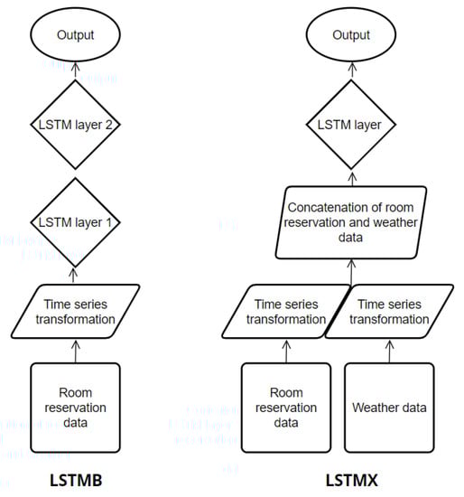
Figure 2.
Schematic representation of the proposed deep learning models for long-term tourism demand forecasting.
4. Data
In this section, we describe the real-world data used for building and evaluating both the proposed and the benchmark tourism demand forecasting models.
4.1. Hotel Data
In order to evaluate both the proposed and the benchmark tourism demand forecasting models, real-world tourism demand data from three hotels in Greece we used. In particular, the dataset used contains room reservation records for each day of past tourist seasons from three different hotels in Greece. We received these data in the form of sets of yield reports from a large tourism management company in Greece. Due to data privacy, we hereafter refer to the three hotels using the terms Hotel A, Hotel B and Hotel C instead of their real names.
Hotel A is a 5-star resort located in a Greek island. Its room reservation data spanned in four seasons, namely from 2013 to 2016, and was delivered as sets of yield reports. Each set corresponded to a season and contained 37 individual reports, where each report was about a specific booking date and contained room reservation records for all arrival days. The number of arrival days in this part of the dataset was 187 from 26 April to 31 October. Hotel B is a 5-star hotel in southern Greece. The room reservation data for this hotel covered four tourist seasons, namely from 2014 to 2017. As in the case of Hotel A, the data from Hotel B were delivered in the form of four sets of yield reports (one for each of the examined seasons), where each set contained 34 reports. Each report was about a specific booking day and contained room reservation records for all 189 arrival days from 24 April to 31 October. Finally, Hotel C is a 5-star hotel in northern Greece. The data from this hotel contained room reservation records from four seasons, namely from 2014 to 2017. The total number of yield reports for each season was 61 and the arrival days were 148 from 12 May to 28 October. It should be noted that the season in this context follows the tourism industry definition and not the calendar definition. This means that when we refer to season we mean the period from April to October of each year. However, we believe that the investigation of our models’ behavior in different calendar seasons will reveal several important characteristics of our approach. Thus, we intend to carry out this investigation as future work.
In all three cases, the room reservation records were organized into time series. In particular, for each arrival day a time series of room reservation values was constructed, where n is the total number of room reservation values for the whole period covered. For n, the following equation holds:
where is the number of seasons covered by the dataset, and L is the number of yield reports per season, i.e., the length of the season. All seasons were the same length for all three hotels. The number of arrival days (i.e., the number of time series for each hotel) is denoted by m. For example, the data from Hotel A covered four seasons (i.e., from 2013 to 2016), and they were delivered in sets of 37 yield reports per season, referring to 187 arrival days. Hence, for Hotel A, a set of time series with size each was constructed. The characteristics of the time series constructed for each hotel are presented in Table 1. Additionally, the room reservation time series for all arrival days of the last seasons of all three hotels (i.e., season 2016 for Hotel A, 2017 for Hotel B and 2017 for Hotel C) are schematically depicted in Figure 3, respectively.

Table 1.
Characteristics of the room reservation time series for all hotels.

Figure 3.
Room reservation time series for all arrival days of the last season of each hotel.
4.2. Weather Data
Apart from the hotel data described above, weather data were also used in the training and the evaluation process of one of the proposed tourism demand forecasting models. In particular, for each of the hotel locations, we gathered values from the five weather variables below:
- Temperature (C)
- Atmospheric pressure (Pa)
- Humidity (%)
- Wind speed (km/h)
- Visibility (m)
The values of these variables were in different time intervals, but we aggregated them, using averages, in to daily intervals. In addition, the total period covered by the weather data was the same as seasons covered by the data for each hotel. These data were gathered from the online weather data repository Weather Underground [45]. As in the case of the hotel data, the weather data were also organized into time series. In particular, for each hotel, a set of five weather time series was constructed, where , and the symbols correspond to temperature, atmospheric pressure, humidity, wind speed and visibility, respectively.
5. Experimental Evaluation
In this section, we describe in detail the overall experimental evaluation framework of the proposed work, along with the corresponding experimental results.
5.1. Experimental Setup
For the evaluation of the proposed tourism demand forecasting models, a set of experiments was designed and performed. Each experiment corresponded to one of the three hotels in the dataset, and its main objective was to measure the forecasting performance of the proposed models and compare it with the performance of benchmark models in the context of a long-term forecasting scenario. This scenario is defined as follows. Given a room reservation time series for an arrival day containing a total of n values from seasons with a season length L each, forecast the room reservations value at the end of next season , or equivalently estimate the value . Repeat this process for all arrival days.
As already mentioned, for each hotel there are four seasons of data. In order to perform the aforementioned experiments, the data were divided into three parts. In particular, the first part (i.e., ) was the training set, the second (i.e., ) the validation set and the third (i.e., ) the test set. The hyperparameter tuning process on the validation data was performed using the grid search method. Moreover, it should be clarified that one single instance of each model was implemented for each hotel, and not a different instance for each arrival day. In addition, given the fact that we are interested in a multi-step-ahead forecasting scenario, we utilized the direct [46,47] multi-step forecasting strategy, instead of the iterative [46,47] or the DirRec [48] strategy. This choice was made because the direct strategy usually gives better results in the long-term forecasting due to the lack of cumulative error [49]. Furthermore, the PPMCC values for all three hotels are presented in Table 2. As shown in the table, the PPMCC values closer to 1 (i.e., perfect positive linear correlation) for all three hotels correspond to the temperature variable, which means that it is the most well correlated weather variable with the tourism variable. Finally, the hyperparameter values of the LSTMB and LSTMX deep learning architectures for the three hotels are summarized in Table 3 and Table 4, respectively.
Table 2.
PPMCC values between the tourism and weather variables for all hotels. The bold values indicate the highest positive correlations identified.
Table 3.
Hyperparameter values of the LSTMB architectures for all hotels.
Table 4.
Hyperparameter values of the LSTMX architectures for all hotels.
In order to measure the forecasting performance of both the proposed and the benchmark models, two forecasting error metrics that are widely used in the tourism demand forecasting literature [50] were utilized, namely, the root mean squared error (RMSE) and the mean absolute percentage error (MAPE). RMSE is defined as the square root of the average of the squared differences between the actual and the predicted values, and it is expressed in the measurement unit of the forecasted variable. Hence, in this case, RMSE was expressed in the number of room reservations (in short ). RMSE is defined by the following equation:
where is the actual value and is the predicted tourism demand value. On the other hand, MAPE is defined as the average of the absolute values of the relative differences between the actual and the predicted values, and it is expressed as a percentage (%). MAPE is defined by the following equation:
where is the actual and is the predicted tourism demand value, respectively.
5.2. Benchmark Models
We compared the forecasting performance of the proposed deep learning models with six benchmark models widely used for tourism demand forecasting, namely, a naive forecasting model, ARIMA, SVR, Holt-Winters exponential smoothing, MLP, and Bayesian Ridge Regression (BRR). In what follows, we provide a brief description for each of these benchmark models.
- Naive forecasting modelIn every time series forecasting task, it is useful to compare the forecasting performance of a new proposed model with that of a simplistic model, e.g., the model whose predicted value for a dependent variable is equal to the current value of the variable, regardless of the forecasting horizon. This naive forecasting model makes its predictions using the following equation:where h is the forecasting horizon. If the forecasting accuracy of a new model is not higher than the accuracy of the naive forecasting model, then the proposed model cannot be considered as useful.
- Autoregressive Integrated Moving AverageThe ARIMA model is one of the most widely used statistical models for time series forecasting in general, as well as for tourism demand forecasting, in particular. The method was popularized by the work of Box and Jenkins [51] in the 1970s. In short, an ARIMA() model is described by the following equation:where p is the autoregressive order, q is the moving average order, d is the order of differencing (i.e., how many times the method of first differences needs to be applied on a time series to make it stationary), are the autoregressive parameters of the model, are the moving average parameters of the model, is the lag operator (i.e., ) and is white noise with zero mean and constant variance. The parameters of the ARIMA model are generally estimated using either the nonlinear least squares method or the maximum likelihood method. When the ARIMA model does not include the moving average component, its autoregressive parameters can be estimated using the ordinary least squares method.
- Support Vector RegressionSupport vector regression (SVR) is the version of the support vector machine (SVM) model for regression problems. Considering as the input vector of the SVR model, its prediction is given by the following equation:where is the prediction for the input vector , w is the parameter vector of the SVR model, b is the bias of the SVR model, and denotes the dot product. Given a set of training samples , the training process of the SVR model can be expressed by the following optimization problem:where is a hyperparameter of the SVR model that serves as a threshold, and in particular, all predictions have to be within an range of the true predictions. In addition, slack variables may be introduced to the problem in order to allow prediction errors to flow out of the range boundaries. The above optimization problem is usually solved using quadratic programming methods such as the method of Lagrange multipliers.
- Holt-Winters Exponential SmoothingThe Holt-Winters exponential smoothing (or triple exponential smoothing) model is a statistical forecasting model. It is a variant of the simple exponential smoothing model, and it takes into account the possibility of trends and seasonality in the time series data. The seasonality in the data can be either additive or multiplicative. We utilized the Holt-Winters exponential smoothing model with multiplicative seasonality, which is described by the following equations:where:
- -
- is the value of the time series at time t;
- -
- is the smoothed value of the constant part of the time series at time t;
- -
- is the estimate of the linear trend part of the time series at time t;
- -
- is the estimate of the seasonal part of the time series at time t;
- -
- is the output of the model at time , where ;
- -
- is the data smoothing factor for which holds;
- -
- is the trend smoothing factor for which holds;
- -
- is the seasonal change smoothing factor for which holds;
- -
- L is the length of the season.
The free parameters of the model, namely, the factors , and , are set explicitly by the analyst of estimated by the data using nonlinear optimization methods (e.g., the Nelder-Mead method [52]). Finally, the initial values and can be estimated in various ways. For example, a formula for the initial trend estimate is the following: - Multilayer PerceptronA multilayer perceptron (MLP) is a class of feedforward ANNs which consist of at least three layers of nodes, namely, the input layer, the output layer and at least one hidden layer. Except for the input layer, all other layers contain neurons with arbitrary activation functions. These activation functions may either be linear or nonlinear, but in the majority of cases, they are nonlinear (e.g., hyperbolic tangent function, logistic function, rectifier linear unit—ReLU, etc.). The input layer of the MLP receives the input vectors, while the hidden and output layers perform computations on these vectors in order to derive new vector representations that will lead to the final predictions. The MLPs are trained using the backpropagation technique in a supervised learning way. Finally, MLPs are considered as universal function approximators [53], and therefore they can be used for regression tasks. Moreover, as classification can be considered as a special case of regression in which the target variable is categorical, the MLPs can also be used for classification tasks. An example architecture of an MLP is shown in Figure 4.
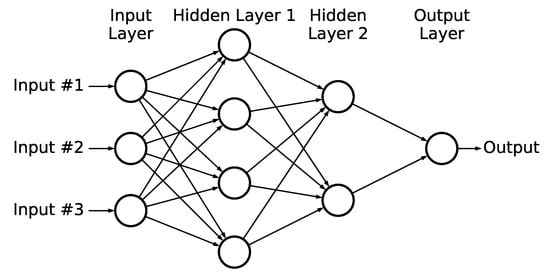 Figure 4. An example MLP architecture.
 - Bayesian Ridge RegressionBayesian ridge regression (BRR) is a probabilistic, regularized model used for regression tasks. The term probabilistic means that instead of trying to find the “best” values of the model parameters in the sense that they minimize the error over training data (or in-sample error), we try to determine the posterior distribution of the model parameters based on the assumption of Gaussian prior distribution and the Bayes theorem. Additionally, the term regularized means that the model integrates parameters that constrain the size of the model parameters. In the BRR, the prior for the model parameters vector w is given by a spherical Gaussian:The priors for and are considered gamma distributions. The estimation of the model is performed by iteratively maximizing the marginal log-likelihood of the data values.
As in the case of the proposed models, the hyperparameter values of the benchmark models were estimated using the grid search method. In particular, regarding the ARIMA model, an ARIMA() model instance was built for each hotel, in which the parameters were estimated using the maximum likelihood estimation method. For the SVR benchmark model, a linear kernel was used for all hotels, and the optimal value of was for Hotel A and Hotel B and for Hotel C. In the case of the Holt-Winters exponential smoothing model, a different instance of the model was built for each arrival day and hotel. Therefore, a different set of optimal values for the parameters , , and was estimated. However, the optimal values of and were constant across all arrival days and hotels and were equal to and 0 respectively. The optimal value of ranged between 0 and . Regarding the MLP, the MLP architecture for Hotel A contained one hidden layer with 128 neurons and was trained using the RMSProp method with batch sizes of 32 and 200 epochs. For Hotel B, the MLP architecture contained one hidden layer with 64 neurons, which was trained using RMSProp with batch sizes of 32 and 200 epochs. Finally, for Hotel C, the MLP architecture contained one hidden layer with 30 neurons and was trained using the RMSProp method with batch sizes of 32 and 100 epochs. In all three cases, the activation function of the hidden neurons was the ReLU; the networks had one input layer with L nodes and one output layer with one neuron and linear activation function. The hyperparameter values of these MLP architectures for the three hotels are summarized in Table 5. Finally, regarding the BRR model, the optimal values of the hyperparameters , , and was for all hotels.
Table 5.
Hyperparameter values of the MLP architectures for all hotels.
5.3. Experimental Results
The forecasting performance results of both the proposed and the benchmark models for all hotels are presented in Table 6 and schematically in Figure 5. As shown in the table, in most cases the proposed deep learning models outperform the benchmark models. Additionally, the LSTMX model that integrates weather data outperforms the LSTMB model in two out of three cases. This result validates the correctness of our assumption that the integration of values from exogenous variables (e.g., temperature) can increase the forecasting accuracy of an LSTM-based tourism demand forecasting model, provided that these variables are well-correlated to the demand variable.
Table 6.
Forecasting performance results of all models for all hotels.

Figure 5.
Schematic depiction of the forecasting performance results (MAPE and RMSE) of all models for all hotels.
Specifically, regarding Hotel A, the proposed deep learning models outperform all benchmark models. In addition, the forecasting performance of the LSTMX model is slightly worse than the performance of the LSTMB model. In the case of Hotel B, the LSTMX model outperforms all benchmark models, while the LSTMB model outperforms all models except the Holt-Winters model. In both cases, LSTMX presents higher forecasting accuracy compared to LSTMB. Finally, in the case of Hotel C, the deep learning models are the best performing models, and the LSTMX model presents again higher forecasting accuracy compared to the LSTMB model. Finally, regarding the benchmark models, the best performing model for Hotel A and Hotel B was the Holt-Winters model and for Hotel C the SVR, while the Holt-Winters had very similar forecasting performance. All aforementioned comparisons between models were made based on the values of the MAPE metric.
The proposed deep learning models exhibit their best forecasting accuracy for Hotel A, which has the most stable room reservation time series for all arrival days in the test period. On the other hand, they exhibit their worst forecasting accuracy for Hotel B, which has the most volatile time series (i.e., time series with the highest variance). To depict this behavior schematically, the time series of long-term forecasts for all arrival days generated by the proposed deep learning models are presented in Figure 6 for Hotel A, Hotel B and Hotel C. As shown in the figures, the models fit very well on the room reservation time series of Hotel A, while presenting differences in some points in the time series of Hotel B and Hotel C. This behavior is a piece of evidence that the forecasting performance of the LSTM-based models deteriorates with the volatility of the time series trying to predict.
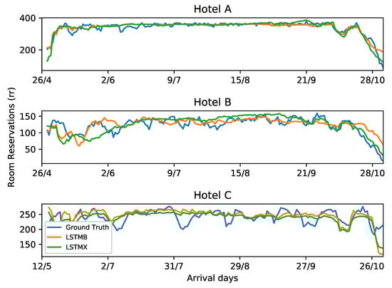
Figure 6.
Time series of the actual and the (long-term) forecasted room reservations generated by the proposed deep learning models for all arrival days of each hotel.
Furthermore, in order to verify that the difference between the forecasting performance of the proposed deep learning models and that of the best performing benchmark model for each hotel is statistically significant, we utilized the Wilcoxon signed-rank test [54]. This test assesses the null hypothesis that two samples of values were drawn from populations having the same distribution, and it can be used in cases where the samples are small and their values cannot be assumed to be normally distributed. In our case, we compared the residuals (i.e., the differences between the actual and predicted demand values) produced by the proposed models and those of the best performing models for each hotel. Due to the disagreement regarding the best performing benchmark model according to the two error metrics, for each hotel we evaluated the best performing model according to both metrics (e.g., for Hotel A, we evaluated both the MLP and the Holt-Winters models). In all cases, the null hypothesis of the test was rejected, and therefore, the difference in forecasting accuracy between the proposed models and the best performing benchmark models can be considered as statistically significant. It should be noted that the sizes of the residual samples can be considered small (i.e., 187, 189, and 148 for Hotel A, Hotel B, and Hotel C, respectively), and their probability distributions also cannot be considered normal, as verified by the application of the Shapiro-Wilk [55] statistical test. Hence, the Wilcoxon signed-rank test is applicable.
As presented in Section 3.4, the LSTMX model integrates data from the temperature weather variable. However, in order to extract more evidence about the impact of the weather data on the forecasting performance of the proposed deep learning architectures, we trained and tested a set of LSTMX(k) models, where and the symbols correspond to atmospheric pressure, humidity, wind speed and visibility, respectively. Each LSTMX(k) model is similar in terms of architecture with the base LSTMX model, but it integrates data from the k weather variable instead of the temperature. The experimental setup for these additional models was exactly the same with the one described in Section 5.1. The forecasting performance results of these models are presented in Table 7. As shown in the table, the base LSTMX model (i.e., temperature) outperforms all LSTM(k) variants for Hotel A and Hotel B, while in the case of Hotel C the LSTMX() and LSTMX(V) present the best performance. While in Hotel A and Hotel B, the new variants of the LSTMX model that integrate data from other exogenous variables do not achieve better results compared to the LSTMB model and the initial LSTMX model, in the case of Hotel C, the two variants outperform both LSTMB and the initial LSTMX. This finding indicates that other models probably exist that might yield even better forecasting performance. Our initial assumption is that these models should either integrate data from multiple exogenous variables (e.g., LSTMX()) or might be ensembles of the existing models. However, more experiments are required to better support this claim, which will be performed as future work.
Table 7.
Forecasting performance results of the LSTMX(k) variants for all hotels.
6. Conclusions
In this paper, we proposed new deep learning architectures for long-term tourism demand forecasting. In particular, the proposed architectures are based on the LSTM network, which is capable of incorporating data from exogenous variables. Two different architectures were implemented, namely one using only historical tourism-related data and another one which, in addition to tourism-related data, also integrates weather data. The proposed models were evaluated on real-world tourism demand data from three hotels in Greece. Based on the experimental results, it was concluded that the proposed models achieve better forecasting performance in all cases compared to six different benchmark models widely used for tourism demand forecasting. In addition, we validated our assumption that the integration of data from exogenous variables (e.g., weather data) in a base deep learning architecture, used for long-term tourism demand forecasting, can significantly improve its performance. Through this work, we experimentally verified our intuition that the integration of data from exogenous variables into a model used for long-term tourism demand forecasting improves its accuracy. We believe that this is an important outcome for the respective scientific community that should be further investigated. Future research directions of this work include the experimentation with different types of exogenous variables (e.g., combinations of variables, demographics, etc.), season-wise experimentation, and model optimization along the lines of the work presented in [38]. Furthermore, we intend to apply the proposed models in similar tourism-related datasets from hotels in other regions of the Mediterranean, such as Italy.
Author Contributions
Conceptualization, A.S. and G.X.; Data curation, A.S. and G.X.; Formal analysis, A.S., G.X. and D.K.; Funding acquisition, D.T.; Investigation, A.S. and G.X.; Methodology, A.S.; Project administration, D.K. and A.S.; Resources, D.T.; Software, G.X. and A.S.; Supervision, A.S.; Validation, A.S. and D.K.; Writing—original draft, G.X.; Writing—review & editing, A.S. All authors have read and agreed to the published version of the manuscript.
Funding
This research was carried out as part of the project «Artificial Intelligence Platform for Dynamic Advertising & Hotel Reservation» (Project code: KMP6-0082081) under the framework of the Action «Investment Plans of Innovation» of the Operational Program «Central Macedonia 2014 2020», that is co-funded by the European Regional Development Fund and Greece.
Data Availability Statement
The data presented in this study are not shared publicly due to legal and copyright restrictions.
Acknowledgments
The authors of the paper would like to thank Andreas Birner and Inova Hospitality Management for the provision of anonymized data presented in this work.
Conflicts of Interest
The authors declare no conflict of interest.
References
- Hayes, D.K.; Miller, A.A. Revenue Management for the Hospitality Industry; Wiley: Hoboken, NJ, USA, 2011. [Google Scholar]
- He, K.; Ji, L.; Wu, C.W.D.; Tso, K.F.G. Using SARIMA-CNN-LSTM approach to forecast daily tourism demand. J. Hosp. Tour. Manag. 2021, 49, 25–33. [Google Scholar] [CrossRef]
- Li, Y.; Cao, H. Prediction for Tourism Flow based on LSTM Neural Network. Procedia Comput. Sci. 2018, 129, 277–283. [Google Scholar] [CrossRef]
- Hsieh, S.C. Tourism Demand Forecasting Based on an LSTM Network and Its Variants. Algorithms 2021, 14, 243. [Google Scholar] [CrossRef]
- Pascanu, R.; Mikolov, T.; Bengio, Y. On the difficulty of training recurrent neural networks. In Proceedings of the 30th International Conference on Machine Learning; Dasgupta, S., McAllester, D., Eds.; PMLR: Atlanta, GA, USA, 2013; Volume 28, pp. 1310–1318. [Google Scholar]
- Zhang, C.; Wang, S.; Sun, S.; Wei, Y. Knowledge mapping of tourism demand forecasting research. Tour. Manag. Perspect. 2020, 35, 100715. [Google Scholar] [CrossRef] [PubMed]
- Schaer, O.; Kourentzes, N.; Fildes, R. Demand forecasting with user-generated online information. Int. J. Forecast. 2019, 35, 197–212. [Google Scholar] [CrossRef]
- Louvieris, P. Forecasting international tourism demand for Greece: A contingency approach. J. Travel Tour. Mark. 2002, 13, 5–19. [Google Scholar] [CrossRef]
- Bokelmann, B.; Lessmann, S. Spurious patterns in Google Trends data—An analysis of the effects on tourism demand forecasting in Germany. Tour. Manag. 2019, 75, 1–12. [Google Scholar] [CrossRef]
- Andrawis, R.R.; Atiya, A.F.; El-Shishiny, H. Combination of long term and short term forecasts, with application to tourism demand forecasting. Int. J. Forecast. 2011, 27, 870–886. [Google Scholar] [CrossRef]
- Li, H.; Goh, C.; Hung, K.; Chen, J.L. Relative climate index and its effect on seasonal tourism demand. J. Travel Res. 2018, 57, 178–192. [Google Scholar] [CrossRef]
- Winters, P.R. Forecasting Sales by Exponentially Weighted Moving Averages. Manag. Sci. 1960, 6, 324–342. [Google Scholar] [CrossRef]
- Gunter, U.; Önder, I. Forecasting international city tourism demand for Paris: Accuracy of uni- and multivariate models employing monthly data. Tour. Manag. 2015, 46, 123–135. [Google Scholar] [CrossRef]
- Pan, B.; Yang, Y. Forecasting Destination Weekly Hotel Occupancy with Big Data. J. Travel Res. 2017, 56, 957–970. [Google Scholar] [CrossRef]
- Li, G.; Wong, K.K.; Song, H.; Witt, S.F. Tourism demand forecasting: A time varying parameter error correction model. J. Travel Res. 2006, 45, 175–185. [Google Scholar] [CrossRef]
- Önder, I. Forecasting tourism demand with Google trends: Accuracy comparison of countries versus cities. Int. J. Tour. Res. 2017, 19, 648–660. [Google Scholar] [CrossRef]
- Li, X.; Pan, B.; Law, R.; Huang, X. Forecasting tourism demand with composite search index. Tour. Manag. 2017, 59, 57–66. [Google Scholar] [CrossRef]
- Chen, J.L.; Li, G.; Wu, D.C.; Shen, S. Forecasting Seasonal Tourism Demand Using a Multiseries Structural Time Series Method. J. Travel Res. 2019, 58, 92–103. [Google Scholar] [CrossRef]
- Baldigara, T.; Mamula, M. Modelling international tourism demand using seasonal arima models. Tour. Hosp. Manag. 2015, 21, 1–31. [Google Scholar] [CrossRef]
- Support vector regression machines. Adv. Neural Inf. Process. Syst. 1997, 1, 155–161.
- Saayman, A.; Botha, I. Non-linear models for tourism demand forecasting. Tour. Econ. 2017, 23, 594–613. [Google Scholar] [CrossRef]
- Hu, M.; Song, H. Data source combination for tourism demand forecasting. Tour. Econ. 2020, 26, 1248–1265. [Google Scholar] [CrossRef]
- Bi, J.W.; Han, T.Y.; Li, H. International tourism demand forecasting with machine learning models: The power of the number of lagged inputs. Tour. Econ. 2020, 28, 3. [Google Scholar] [CrossRef]
- Claveria, O.; Torra, S. Forecasting tourism demand to Catalonia: Neural networks vs. time series models. Econ. Model. 2014, 36, 220–228. [Google Scholar] [CrossRef]
- Claveria, O.; Monte, E.; Torra, S. Tourism demand forecasting with neural network models: Different ways of treating information. Int. J. Tour. Res. 2015, 17, 492–500. [Google Scholar] [CrossRef]
- Akin, M. A novel approach to model selection in tourism demand modeling. Tour. Manag. 2015, 48, 64–72. [Google Scholar] [CrossRef]
- Hassani, H.; Silva, E.S.; Antonakakis, N.; Filis, G.; Gupta, R. Forecasting accuracy evaluation of tourist arrivals. Ann. Tour. Res. 2017, 63, 112–127. [Google Scholar] [CrossRef]
- Lin, C.J.; Chen, H.F.; Lee, T.S. Forecasting Tourism Demand Using Time Series, Artificial Neural Networks and Multivariate Adaptive Regression Splines: Evidence from Taiwan. Int. J. Bus. Adm. 2011, 2, 14–24. [Google Scholar] [CrossRef]
- Teixeira, J.; Fernandes, P. Tourism time series forecast with artificial neural networks. Tékhne 2014, 12, 26–36. [Google Scholar] [CrossRef]
- Constantino, H.; Fernandes, P.; Teixeira, J. Tourism demand modelling and forecasting with artificial neural network models: The Mozambique case study. Tékhne 2016, 14, 113–124. [Google Scholar] [CrossRef]
- Lijuan, W.; Guohua, C. Seasonal SVR with FOA algorithm for single-step and multi-step ahead forecasting in monthly inbound tourist flow. Knowl.-Based Syst. 2016, 110, 157–166. [Google Scholar] [CrossRef]
- Zhang, B.; Pu, Y. Study on Tourist Volume Forecasting Based on ABA-SVR Model Within Network Environment. In 3rd International Conference on Judicial, Administrative and Humanitarian Problems of State Structures and Economic Subjects; Atlantis Press: Dordrecht, The Netherlands, 2018; Volume 252, pp. 460–466. [Google Scholar] [CrossRef]
- Claveria, O.; Monte, E.; Torra, S. Combination forecasts of tourism demand with machine learning models. Appl. Econ. Lett. 2016, 23, 428–431. [Google Scholar] [CrossRef]
- y Gómez, M.M., Escalante, H.J., Segura, A., de Dios Murillo, J., Eds.; Advances in Artificial Intelligence—IBERAMIA 2016. In Proceedings of the 15th Ibero—American Conference on AI, San José, Costa Rica, 23–25 November 2016; Volume 1022, pp. 201–211. [Google Scholar] [CrossRef]
- Cuhadar, M.; Cogurcu, I.; Kukrer, C. Modelling and Forecasting Cruise Tourism Demand to Izmir by Different Artificial Neural Network Architectures. Int. J. Bus. Soc. Res. 2014, 4, 12–28. [Google Scholar]
- Polyzos, S.; Samitas, A.; Spyridou, A.E. Tourism demand and the COVID-19 pandemic: An LSTM approach. Tour. Recreat. Res. 2021, 46, 175–187. [Google Scholar] [CrossRef]
- Kulshrestha, A.; Krishnaswamy, V.; Sharma, M. Bayesian BILSTM approach for tourism demand forecasting. Ann. Tour. Res. 2020, 83, 102925. [Google Scholar] [CrossRef]
- Waseem, M.; Lin, Z.; Liu, S.; Jinai, Z.; Rizwan, M.; Sajjad, I.A. Optimal BRA based electric demand prediction strategy considering instance-based learning of the forecast factors. Int. Trans. Electr. Energy Syst. 2021, 31, e12967. [Google Scholar] [CrossRef]
- Law, R.; Li, G.; Fong, D.K.C.; Han, X. Tourism demand forecasting: A deep learning approach. Ann. Tour. Res. 2019, 75, 410–423. [Google Scholar] [CrossRef]
- Sun, S.; Li, Y.; Guo, J.-E.; Wang, S. Tourism Demand Forecasting: An Ensemble Deep Learning Approach. arXiv 2021, arXiv:stat.AP/2002.07964. [Google Scholar] [CrossRef]
- Wang, J.; Duggasani, A. Forecasting hotel reservations with long short-term memory-based recurrent neural networks. Int. J. Data Sci. Anal. 2020, 9, 77–94. [Google Scholar] [CrossRef]
- Zipser, D.; Williams, R.J. Gradient-Based Learning Algorithms for Recurrent Networks and Their Computational Complexity. In Backpropagation: Theory, Architectures, and Applications; Psychology Press: London, UK, 1995; pp. 433–486. [Google Scholar]
- Hochreiter, S.; Schmidhuber, J. Long Short-Term Memory. Neural Comput. 1997, 9, 1735–1780. [Google Scholar] [CrossRef]
- Tieleman, T.; Hinton, G. Lecture 6.5-rmsprop: Divide the gradient by a running average of its recent magnitude. COURSERA Neural Netw. Mach. Learn. 2012, 4, 26–31. [Google Scholar]
- Weather Underground. 2019. Available online: https://www.wunderground.com/ (accessed on 10 October 2021).
- Sorjamaa, A.; Hao, J.; Reyhani, N.; Ji, Y.; Lendasse, A. Methodology for long-term prediction of time series. Neurocomputing 2007, 70, 2861–2869. [Google Scholar] [CrossRef]
- Hamzaçebi, C.; Akay, D.; Kutay, F. Comparison of direct and iterative artificial neural network forecast approaches in multi-periodic time series forecasting. Expert Syst. Appl. 2009, 36, 3839–3844. [Google Scholar] [CrossRef]
- Sorjamaa, A.; Lendasse, A. Time series prediction using DirRec strategy. In Proceedings of the ESANN, Bruges, Belgium, 26–28 April 2006. [Google Scholar]
- Ji, Y.; Hao, J.; Reyhani, N.; Lendasse, A. Direct and recursive prediction of time series using mutual information selection. Lect. Notes Comput. Sci. 2005, 3512, 1010–1017. [Google Scholar] [CrossRef]
- Guizzardi, A.; Stacchini, A. Real-time forecasting regional tourism with business sentiment surveys. Tour. Manag. 2015, 47, 213–223. [Google Scholar] [CrossRef]
- Box, G.; Jenkins, G. Time Series Analysis: Forecasting and Control; Revised Edition, Holden Day, San Francisco; Wiley: Hoboken, NJ, USA, 1976. [Google Scholar]
- Nelder, J.A.; Mead, R. A Simplex Method for Function Minimization. Comput. J. 1965, 7, 308–313. [Google Scholar] [CrossRef]
- Cybenko, G. Approximation by superpositions of a sigmoidal function. Math. Control Signals Syst. 1989, 2, 303–314. [Google Scholar] [CrossRef]
- Wilcoxon, F. Individual Comparisons by Ranking Methods. Biometrics 1945, 1, 196–202. [Google Scholar]
- Shapiro, A.S.S.; Wilk, M.B. Biometrika Trust An Analysis of Variance Test for Normality (Complete Samples). Biometrika 1965, 52, 591–611. [Google Scholar] [CrossRef]


Publisher’s Note: MDPI stays neutral with regard to jurisdictional claims in published maps and institutional affiliations. |
© 2022 by the authors. Licensee MDPI, Basel, Switzerland. This article is an open access article distributed under the terms and conditions of the Creative Commons Attribution (CC BY) license (https://creativecommons.org/licenses/by/4.0/).