Abstract
To obtain a more comprehensive knowledge of the surface electric field distribution of composite insulators, a three-dimensional (3D) simulation model of a 10 kV FXBW4-10/70 composite insulator was established, and the distribution of the axial and radial electric fields on the surface of the insulator under normal, damaged, internal defect, and fouling fault conditions were calculated and analyzed based on the finite element method. The results showed that the axial and radial electric field distributions on the surfaces of the normal composite insulators were “U” shaped, the radial electric field at the damaged location had a greater change than the axial electric field, and both the axial and radial electric fields at the internal defect location increased significantly. For the insulator covered with NaCl conductive fouling, the axial electric fields at the high-voltage (HV) and low-voltage (LV) ends showed a greater change. The results can provide a basis for the fault identification of composite insulators and the optimal design of insulation structures.
1. Introduction
Compared to conventional ceramic and glass insulators, composite insulators are widely used in high-voltage (HV) transmission lines due to their excellent performance. However, the composite insulator is usually subjected to damage, internal defects, and fouling faults during operation. Generally, internal defects are difficult to identify based on the appearance, but they are also the most dangerous. When a composite insulator skirt is broken, the creepage distance is reduced, and the electric field strength is concentrated at the point of the damage, resulting in the accelerated aging of the polymer material and a reduced service life. At the same time, the broken umbrella skirt intensifies the uneven distribution of the potential, leading to a drop in the flashover electrical field and, in weather such as haze, a very easy fouling flashover, resulting in huge losses [1,2,3,4,5,6]. When the sheath seal of composite insulators is defective, partial discharges are prone to occur at the intersection of the mandrel and sheath, as well as defects such as air gaps and moisture left inside the mandrel. Long-term partial discharges produce charred channels that gradually develop along the mandrel and reduce the total insulation length. These discharges severely corrode the mandrel, separating the mandrel from the sheath and, in severe cases, causing the mandrel to fracture [7,8,9,10,11,12]. As composite insulators are exposed to the atmosphere for a long time, various soot, dust, waste, and other dirt particles generated by industries slowly move to the insulator surface under the action of the airflow, and after long-term accumulation, they form a dirt layer on the insulator surface. The existence of the dirt layer changes the electrical conductivity of the insulator surface and affects the distribution of the electrical charge on the insulator surface. In addition, the accumulated electrical charge on the insulator surface leads to the accumulation of charge on the insulator surface, resulting in a more uneven distribution of the electric field, possibly even leading to serious flashover on the insulator surface. When an insulator flashover occurs, it may lead to the interruption of power supply and, in severe cases, may even cause widespread and extensive power outages, affecting the safe and stable operation of HV transmission and distribution lines [13,14,15,16,17,18]. Therefore, it is important to clearly understand the surface electric field distribution of the faulty composite insulator.
In [1], the flashover characteristics of composite insulators with umbrella skirt damage at 35 kV, 110 kV, and 220 kV voltage levels were investigated. In [5], by combining electric field simulation and aging test results, the axial electric field of the aging damage of umbrella skirts of 110 kV composite insulators at different locations and the effect of the axial electric field distribution on the aging of the composite insulators were analyzed and investigated. In [8], the effects of internal defects at different locations on the axial and radial electric field distributions of the 69, 110, and 230 kV composite insulators were analyzed. In [10], the axial electric field distribution characteristics of 500 kV composite insulators with defects on the core bar surface were analyzed. In [15,16], the flashover performance of 500 kV composite insulators with different contaminants was investigated. In [18], the formation of dry bands on the surface of 110 kV composite insulators and the effects of contaminants on the electric field of the insulators were analyzed. In [19], a 500 kV composite insulator model with internal defects was established, and the axial electric field distribution of the composite insulator was calculated. The results showed that the electric field value, across all the defects, increased significantly. In [20], based on the finite element method, the influence of the voltage divider ring on the axial electric field distribution of 220 kV and 500 kV composite insulators was analyzed. The results showed that the voltage divider ring can reduce the electric field of a high-voltage terminal insulator. In [21], it was concluded that the local electric field on the surface of 110 kV composite insulators becomes distorted after high-voltage end sheath aging and moisture absorption. In [22], the electric field distribution of composite insulators of a 115 kV AC voltage was illustrated, and the influence of the electric field distribution on the performance of the composites was discussed. In [23], the ANSYS was used to analyze the axial electric field distribution of the 110 kV composite insulator, and it was concluded that the aging degree of the high-voltage end is the most significant, the low-voltage side is the second, and the middle part has the weakest degree of aging.
From the analysis above, we can see that the current research is mainly focused on the axial electric field distribution on the surface of composite insulators above 110 kV, while there is little research on the radial electric field distribution on the surfaces of composite insulators, especially those below 110 kV. This paper presents a numerical simulation and analysis of both the axial and radial electric field distributions on the surface of a 10 kV composite insulator under normal, damaged, internal defect, and fouling fault conditions using the finite element method. The effects of the damage and defect locations and NaCl fouling on the axial and radial electric fields of the composite insulator are analyzed, respectively. The distribution patterns of the axial and radial electric fields at the HV end and the low-voltage (LV) end and the fault positions on the surface of the composite insulator are shown. All the results can provide a basis for the optimization of the design and fault identification of composite insulators.
2. Simulation Model Development and Parameter Settings
2.1. Simulation Model
The study object is a rod-type suspension composite insulator, type FXBW 4-10/70, which is mainly used for overhead lines and substations in AC power systems, with a rated voltage of 10–330 kV and a frequency not exceeding 100 Hz. The structural dimensions of the composite insulator are shown in Table 1. As the simplified composite insulator is an axisymmetric structure from a macroscopic point of view, many scholars have also used a two-dimensional (2D) model to analyze the electric field and potential of the insulator. However, only one directional cloud picture profile can be obtained through 2D electric field analysis. However, the use of a three-dimensional (3D) model can reflect the results of calculations in multiple directions and can take into account the asymmetry caused by internal defects and damage, rendering the simulation results more realistic and accurate [3]. Therefore, a 3D model of the composite insulator was developed by using the finite element simulation software COMSOL Multiphysics to analyze and calculate the electric field distribution.

Table 1.
Composite insulator parameters.
Since the electric field distribution throughout the insulator is an unbounded domain, to solve the electric field distribution, it must first be transformed into a finite domain. When the domain is set to be larger than 300 mm × 300 mm × 420 mm, the electric field around of the insulator remains unchanged. Therefore, a 300 mm × 300 mm × 420 mm cuboid domain is established during the calculation. Almost none of the silicone rubber electrical insulating properties are affected by temperature. Thus, ignoring the influence of temperature, the model is established at a constant temperature of 293.15 K.
The model consists of an umbrella skirt, mandrel, air, and metal fittings, where the mandrel is mainly epoxy resin glass fiber (internal insulation), the umbrella skirt (sheath, external insulation, protection of the core bar) is formed of silicone rubber, and the metal fittings (upper and lower coupling flanges) are steel. The relative dielectric constant and conductivity of each material are shown in Table 2.
Table 2.
Physical parameters of each material.
2.2. Electric Field Control Equations
Considering that the electric field on the surface of the composite insulator is generated by the current in the wire, for the power frequency of 50 Hz, the corresponding wavelength is 6000 km, which is much larger than the physical size of the insulator. Therefore, in simulations, the field distribution can be considered as the electrostatic field.
For the HV AC transmission, frequency domain analysis is used for the electric field module, with the control equations given in Equation (1):
In Equation (1), J (A/m2) is the total current density, Qj © is the charge density, σ (S/m) is the electrical conductivity, and Je (A/m2) is the external current density.
The frequency is set to 50 Hz, and the boundary condition at the HV end is set to V1 = Vi = 10 kV, and the voltage boundary condition at the low-voltage (LV) end is set to V2 = 0.
3. Electric Field Distribution Analysis of the Composite Insulators
In order to compare and analyze the electric field distribution of the faulty composite insulator with that of the normal composite insulator, the electric field and potential distribution around the sheath and mandrel of the normal composite insulator are first calculated. The relative permittivity and conductivity are shown in Table 2. As shown in Figure 1, the bottom end of the composite insulator is set as the HV end, and the top end is set as the LV end, which are numbered vertically from the HV end to the LV end (from bottom to top). The umbrella skirts are marked in the order from 1 to 4, and the middle positions of the two adjacent skirts are marked in the order from “a” to “e”, respectively. For example, “a” stands for the position between the HV end and the first piece of the umbrella skirts, “b” stands for the middle position between the first piece of the umbrella skirts and the second piece of the umbrella skirts, “c” stands for the middle position between the second piece of the umbrella skirts and the third piece of the umbrella skirts, “d” stands for the middle position between the third piece of the umbrella skirts and the forth piece of the umbrella skirts, and “e” stands for the middle position between the forth piece of the umbrella skirts and the HV end.
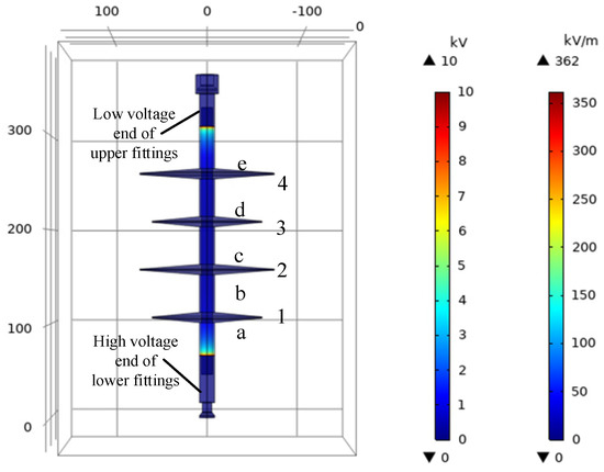
Figure 1.
Electric field potential distribution of the normal composite insulator.
As can be seen from Figure 1, the electric field distribution from the HV end to the LV end is not uniform, and the electric field on the surface of the composite insulator is higher at the HV and LV ends, while the field in the middle position is relatively lower. This is due to the fact that the electric field is mainly concentrated at the intersection of the root of the umbrella skirt with the hardware fittings. The maximum axial electric field is 361.899 kV/m, which occurs near the HV end of the fixture, and the maximum axial electric field near the LV end fixture is 333.587 kV/m. The HV and LV ends of the mandrel and sheath are in a long-term, high-field-strength electromagnetic environment, which can easily lead to partial discharges and, in severe cases, even insulator fracture and breakdown. Therefore, compared to the central part of the insulator, damage to the sheath at the HV and LV ends is more likely to lead to partial discharges, accelerating the aging of the insulating rubber and reducing the electrical strength of the insulator.
3.1. Electric Field on the Surface of a Damaged Composite Insulator
Considering that the damage of the composite insulator sheath is generally caused by bird pecking, wind erosion, rubber aging, etc., most of the damage is minor. On the other hand, the damaged area of the insulator sheath comes into contact with the air. Therefore, in the simulation, the damaged of the composite insulator sheath is established as an air gap with a length of 5 mm, width of 1 mm, and depth of 1 mm [2,3], as shown in Figure 2f. As shown in Figure 2a–e, in order to study the distribution characteristics of the electric field on the surface of the composite insulator with sheath damage at different locations, the damages are established at the “a–e” locations on the surface of the insulator. The cloud diagram of the electric field distribution on the surface of the composite insulator when the sheath is damaged at position “a” is shown in Figure 3. The axial and radial electric field distribution curves of the surface of the normal and damaged composite insulators are shown in Figure 4 and Figure 5. The x-axis stands for the distance along the axial field of the composite insulator, which starts with the intersection of the HV end with the sheath (at 66 mm) and ends with the intersection of the LV end with the sheath (at 310 mm).
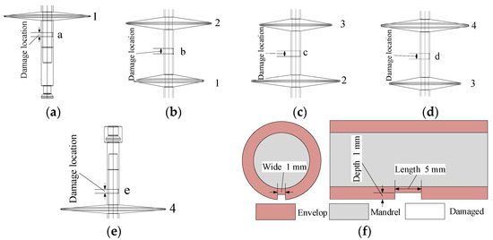
Figure 2.
Calculation model of the composite insulator damaged at: (a) position “a”; (b) position “b”; (c) position “c”; (d) position “d”; and (e) position “e”; (f) model of the damage zone.
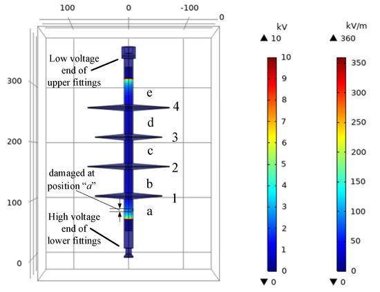
Figure 3.
Electric field potential distribution of the damaged composite insulator at position “a”.
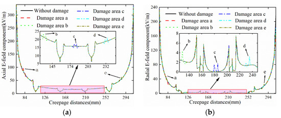
Figure 4.
Distribution curves of the surface of the damaged composite insulator: (a) axial electric field; (b) radial electric field.
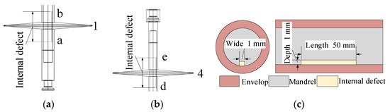
Figure 5.
Calculation model of the composite insulators with internal defects: (a) between “a” − “b”; (b) between “d” − “e”; (c) the internal defect model.
As shown in Figure 4a, when the sheath of the composite insulator is damaged at positions “a” to “e”, the higher axial electric field strength is located near the HV and LV ends of the insulator, while the electric field strength of the middle part of the insulator is relatively lower. The electric field of the whole insulator is distributed in a “U” shape on the surface, and there is a slight distortion in the axial electric field at the locations of the damaged sheath. Furthermore, when the sheath of the composite insulator is damaged on the HV and LV sides (such as the “d” and “e” positions), the increase in the electric field at the damage location is relatively obvious, while when the sheath is damaged in the middle (such as the “b”, “c”, and “d” positions), the electric field change is less significant.
As shown in Figure 4b, when the composite insulator sheath is damaged at positions “a” to “e”, the radial electric field of the composite insulator is higher near the HV end and LV end, while the field in the middle position is relatively lower, but there is a rising distortion at the damaged positions. Compared with the axial electric field on the surface of the composite insulator, the overall reduction in the electric field is evident in the radial electric field strength at the LV end of the damaged composite insulator.
Furthermore, the magnitudes of the axial and radial electric fields on the surface of the insulator at the HV end, LV end, and the damaged location are calculated when there is damage at positions “a” to “e”. The results are shown in Table 3.
Table 3.
Calculation results of the electric field on the surface of the damaged composite insulator.
As shown in Table 3, the maximum axial electric fields Emax(a) on the surface of a normal composite insulator are, respectively, 337.307 kV/m and 333.587 kV/m at the HV and LV ends. When a damaged fault occurs at position “a”, the Emax(a) on the surface of the HV and LV ends are, respectively, 334.327 kV/m and 328.908 kV/m, and the Emax(a) on the surface of the fault location is 96.31 kV/m, whereas the Emax(a) on the surface of the normal composite insulator at this location is 87.323 kV/m. Compared to the normal composite insulator, the maximum axial electric field strengths on the surface of the HV end and LV end are decreased by 0.88% and 1.40%, respectively, while the maximum axial electric field strength on the surface of the faulty position is increased by 10.29%.
When a damaged fault occurs at position “b”, the Emax(a) on the surface of the HV and LV ends are, respectively 336.542 kV/m and 333.347 kV/m, and the Emax(a) on the surface of the fault location is 23.512 kV/m, whereas the Emax(a) on the surface of the normal composite insulator at this location is 21.626 kV/m. Compared to the normal composite insulator, the maximum axial electric field strengths on the surface of the HV and LV ends are decreased, respectively, by 0.23% and 0.07%, and the maximum axial electric field strength on the surface of the fault location is increased by 8.72%.
When a damaged fault occurs at position “c”, the Emax(a) on the surface of the HV and LV ends are 336.849 kV/m and 334.831 kV/m, respectively, and the Emax(a) on the surface of the fault location is 17.213 kV/m, while the Emax(a) on the surface of the normal composite insulator at this location is 15.828 kV/m. Compared to the normal composite insulator, the Emax(a) on the surface of the HV and LV ends are decreased by 0.14% and increased by 0.37%, respectively, while the Emax(a) on the surface of the fault location is increased by 8.75%.
When a damaged fault occurs at position “d”, the Emax(a) on the surface of the HV and LV ends are 339.089 kV/m and 333.466 kV/m, respectively, and the Emax(a) on the surface of the fault location is 21.020 kV/m, whereas the Emax(a) on the surface of the normal composite insulator at this location is 19.153 kV/m. Compared to the normal composite insulator, the Emax(a) on the surface of the HV and LV ends are increased by 0.53% and decreased by 0.04%, respectively, and the Emax(a) on the surface of the fault location is increased by 9.75%.
When a damaged fault occurs at position “e”, the Emax(a) on the surface of the HV and LV ends are 339.067 kV/m and 328.160 kV/m, respectively, and the Emax(a) on the surface of the fault location is 62.424 kV/m, whereas the Emax(a) on the face of the normal composite insulator at this location is 55.672 kV/m. Compared to the normal composite insulator, the Emax(a) on the surface of the HV and LV ends are increased by 0.52% and decreased by 1.63%, respectively, while the maximum axial electric field intensity on the surface at the fault location is increased by 12.13%.
From the above, it can be seen that the change in the axial electric field intensity on the surface of the composite insulator at the HV and LV ends is not very obvious when the damage is slight. However, the electric field intensity at the damaged position is on the rise. The closer the damage is to the HV and LV ends, the more pronounced the change in the axial electric field strength will be.
Moreover, from Table 3, it can be concluded that the maximum radial electric fields Emax(r) on the surface of the normal composite insulator at the HV end and LV end are 212.661 kV/m and 216.942 kV/m, respectively.
When there is a damaged fault at position “a”, the Emax(r) on the surface of the HV end and LV end are 194.329 kV/m and 151.437 kV/m, respectively, and the Emax(r) on the surface of the fault position is 50.063 kV/m, while the Emax(r) on the surface of the normal composite insulator at this position is 47.138 kV/m. Compared to the normal composite insulator, the Emax(r) on the HV and LV ends are decreased by 8.62% and 30.19%, respectively, while the Emax(r) on the fault location is increased by 6.21%.
When a damaged fault occurs at location “b”, the Emax(r) on the surface of the HV and LV ends, respectively, are 235.036 kV/m and 184.974 kV/m, and the Emax(r) on the surface of the fault location is 4.3771 kV/m, while the Emax(r) on the surface of the normal composite insulator at this location is 2.356 kV/m. Compared to the normal composite insulator, the Emax(r) on the surface of the HV and LV ends, respectively, are increased by 10.52% and decreased by 14.74%, while the Emax(r) on the surface at the fault location is increased by 85.73%.
When a damaged fault occurs at position “c”, the Emax(r) on the surface of the HV and LV ends, respectively, are 234.650 kV/m and 183.868 kV/m, and the Emax(r) on the surface of the fault location is 1.8166 kV/m, whereas the Emax(r) on the surface of the normal composite insulator at this location is 0.085 kV/m. Compared to the normal composite insulator, the Emax(r) on the surface at the HV and LV ends, respectively, are increased by 10.34% and decreased by 15.25%, while the Emax(r) on the surface at the fault location is increased by 2029.88%.
When a damaged fault occurs at position “d”, the Emax(r) on the surface of the HV and LV ends, respectively, are 232.658 kV/m and 185.500 kV/m, and the Emax(r) on the surface of the fault location is 3.2196 kV/m, whereas the Emax(r) on the surface of the normal composite insulator at this location is 1.4448 kV/m. Compared to the normal composite insulator, the Emax(r) on the surface of the HV and LV ends, respectively, are increased by 9.40% and decreased by 14.49%, and the Emax(r) on the surface at the fault location is increased by 122.84%.
When a damaged fault occurs at position “e”, the Emax(r) on the surface of the HV end and LV end, respectively, are 232.681 kV/m and 170.861 kV/m, and the Emax(r) on the surface of the fault location is 25.370 kV/m, while the Emax(r) on the face of the normal composite insulator at this location is 21.269 kV/m. Compared to the normal composite insulator, the Emax(r) on the surface of the HV and LV ends are increased by 9.41% and decreased by 21.24%, respectively, while the Emax(r) on the surface at the fault location is increased by 19.28%.
It can be seen that the change in the radial electric field intensity on the surface of the composite insulator at the HV and LV ends is not very obvious when it is slightly damaged but increases at the damaged position. The radial electric field intensity changes the most when location “e” is damaged. This is due to the fact that the position “e” is the middle of the composite insulator, and the radial electric field at this position is very small.
3.2. Electric Field Distribution on the Surface of a Composite Insulator with Internal Defects
When the defects appear inside the composite insulator, its effective insulation distance will be reduced, which causes the insulation performance to decrease, thus leading to an increase in the probability of insulator discharge and flashover. The internal defects mainly appear in the contact position between the mandrel and the sheath of the umbrella skirt and the contact position between the metal fitting and the sheath of the umbrella skirt. The internal defects are most commonly generated at the HV and LV ends, where the mandrel and the sheath of the umbrella skirt are in contact, and are mainly manifested by water infiltration from the external environment, as shown in [7,8,9], which focus on the effect of water immersion on the electric field distribution characteristics of composite insulators.
The internal defects are usually located at the HV and LV ends, where the electric field strength is the highest, and it can be noted that the defect length is usually set as 1.5~20% of the length of the composite insulator [7,8]. As shown in Figure 5c, in this simulation, a water column with a length of 50 mm, a width of 1 mm, and a depth of 1 mm was used to simulate the internal defect of the composite insulator (the length was 13.6% that of the composite insulator). Internal defects were established to simulate the defects inside the composite insulator located between “a” and “b” and between “d” and “e”, respectively, as shown in Figure 5a,b.
Figure 6 shows the electric field distribution between the composite insulator “a” and “b” positions, where an internal defect occurs. The calculated axial and radial electric field intensity distribution curves of the composite insulator on the surface at the HV end, LV end, and the location of the internal defects are shown in Figure 7a,b.
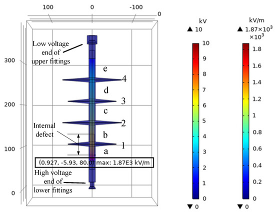
Figure 6.
Electric field potential distribution of the composite insulators with internal defects between “a” − “b”.
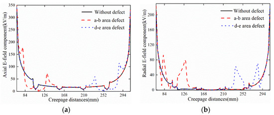
Figure 7.
Distribution curves of the surface of the composite insulator with internal defects: (a) axial electric field; (b) radial electric field.
As shown in Figure 7a, when the internal defects are present between the composite insulator sheath “a” and “b” positions and between the “d” and “e” positions, the axial electric field is higher at the HV and LV ends of the insulator and increases at the defect locations. A significant increase in the axial electric field strength can also be observed at the beginning and end of the defect, but there is a relatively lower field strength at the intermediate locations. This is due to the increased local electric field caused by the presence of the internal defect. The axial electric field intensity at the defect locations rises and then falls. In addition, it can also be observed that the axial electric field intensity is higher in the case of the defects on the HV side than the defects on the LV side. This is due to the fact that the electric field strength on the LV side is inherently low.
As shown in Figure 7b, when the internal defects appear between the composite insulator sheath “a” and “b” positions and between the “d” and “e” positions, the radial electric field at the HV end of the composite insulator has a slight increase, but at the LV end, it has a slight decrease. This is because there is a significant distortion at both ends of the defects, and the radial electric field intensity at the defect location is an “M”-type distribution, while the field intensity at the other locations is relatively lower.
The values of the axial and radial electric fields on the surface of the composite insulator at the HV end, the LV end, and location of the internal defects were calculated when the internal defects existed between “a” and “b” and between “d” and “e”. The results are shown in Table 4.
Table 4.
Calculation results of the electric field in the axial direction for the composite insulator with internal defects.
From Table 4, it can be concluded that the Emax(a) on the surface of the composite insulator, respectively, are 357.462 kV/m and 332.584 kV/m at the HV and LV ends when there is an internal defect between “a” and “b”. The Emax(a) on the surface of the defective zone is 180.064 kV/m, while the Emax(a) on the surface of the normal composite insulator in this zone is 92.136 kV/m. Compared to the normal composite insulator, the Emax(a) on the surface of the high-voltage HV and LV ends are increased, respectively, by 5.98% and decreased by 0.30%, while the Emax(a) on the surface of the defective zone is increased by 95.43%.
The Emax(a) on the surface of the composite insulator are 338.670 kV/m and 331.593 kV/m at the HV and LV ends, respectively, when an internal defect occurs between “d” and “e”. The Emax(a) on the surface of the defective zone is 114.394 kV/m, while the Emax(a) on the surface of the normal composite insulator in this zone is 59.523 kV/m. Compared to the normal insulators, the Emax(a) on the surface of the HV and LV ends are increased by 0.40% and decreased by 0.60%, respectively, and the Emax(a) on the surface of the defective zone is increased by 92.18%.
It can be seen that the change in the axial electric field intensity at the HV and LV ends is not significant when the internal defects are present, but the electric field intensity increases by more than 90% in the defective zone.
The Emax(r) on the surface of the composite insulator are 224.113 kV/m and 200.239 kV/m at the HV and LV ends, respectively, when an internal defect occurs between “a” and “b”. The Emax(r) on the surface of the defective zone is 92.612 kV/m, while the Emax(r) on the surface of the normal composite insulator in this zone is 39.76 kV/m. Compared to the normal composite insulator, the Emax(r) on the surface of the defective zone are increased by 5.39% and decreased by 7.70%, respectively. Compared to the normal composite insulator, the Emax(r) on the surface of the HV and LV ends, respectively, are increased by 5.39% and decreased by 7.70%, and the Emax(r) on the surface of the defective zone is increased by 132.91%.
The Emax(r) on the surface of the composite insulator are 206.118 kV/m and 224.029 kV/m at the HV and LV ends, respectively, when internal defects are present between “d” and “e”. The Emax(r) on the surface of the defective zone is 71.187 kV/m, while that on the surface of the normal composite insulator in this zone is 19.569 kV/m. Compared to the normal insulators, the Emax(r) on the surface of the HV and LV ends, respectively, are decreased by 3.08% and increased by 3.27%, and that on the surface of the defective interval is increased by 263.77%.
It can be seen that the radial electric field at the HV and LV ends varies within a 10% range when internal defects are present but increases by more than a factor of one in the defective zone.
3.3. Electric Field Distribution on the Surface of a Fouled Composite Insulator
The presence of the fouling layer changes the surface electrical conductivity of the insulator and causes charge build-up on the insulator surface, which results in the distortion of the electric field on the insulator surface. According to the Chinese national standard GB/T 4585-2004, for the artificial fouling testing of high-voltage insulators for AC systems, considering that NaCl is one of the main components of insulator surface fouling [15,16], the fouling layer is set in the simulation to be NaCl, with a conductivity of 1.28, uniformly covering the insulator sheath surface, with a thickness of 1 mm [14,15].
Figure 8 shows the electric field distribution on the surface of the insulator, with the NaCl covered. From Figure 8, it can be seen that there is a significant reduction in the electric field strength on the surface of the fouled composite insulator at the HV and LV ends.
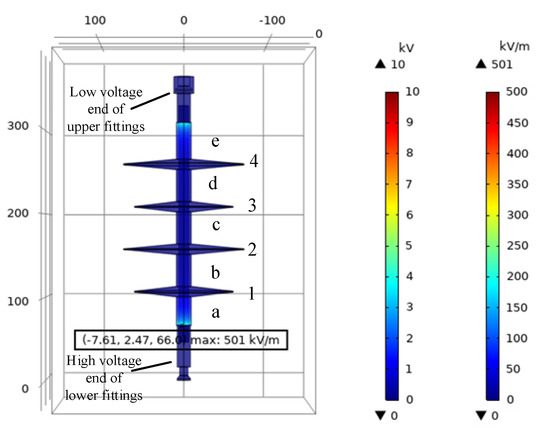
Figure 8.
Electric field potential distribution of the composite insulators covered with the NaCl fouling.
Figure 9a shows the axial electric field distribution curves of the normal and fouled composite insulators. As can be seen from Figure 9a, the Emax(a) on the surface of the HV end of the fouled composite insulator is 186.878 kV/m, which is 44.60% lower than that of the normal insulator. The Emax(a) on the LV end of the fouled composite insulator is 180.201 kV/m, which is 45.98% lower than that of the normal insulator. It is evident that when a fouled layer is present on the surface of the composite insulator, the Emax(a) on the surface of both the HV and LV ends is reduced by more than 40%.
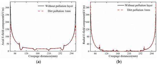
Figure 9.
Distribution curves on the surface of the fouled composite insulator: (a) axial electric field; (b) radial electric field.
Figure 9b shows the radial electric field distribution curves of the normal and fouled composite insulators. As can be seen from Figure 9b, the Emax(r) on the HV end of the fouled composite insulator is 269.725 kV/m, compared with the normal insulator, whose Emax(r) at the HV end is increased by 26.83%. The Emax(r) at the LV end of the fouled composite insulator is 267.746 kV/m, compared with the normal insulator, whose Emax(r) at the LV end is increased by 23.42%. It is clear that when the surface of the composite insulator is fouled, the Emax(r) on the surface of both the HV and LV ends increases by more than 20%.
3.4. Electric Field Distribution on the Surfaces of the Composite Insulators with Different Faults
Existing research has focused on the analysis of the axial electric field distribution on the surfaces of insulators, with little research on the radial electric field distribution. In this paper, the axial and radial electric fields on the surfaces of a normal composite insulator and faulty composite insulators with three different defects were compared and analyzed. The combination of the axial and radial electric field strengths of the composite insulators can be used to provide a basis for determining the faults of the composite insulators.
As shown in Table 5, the maximum differences in the electric field strength in the surface axial and radial directions of the normal composite insulators and faulty composite insulators were calculated. When the composite insulator has a damaged fault, the axial electric field varies between 0.14% and 0.88% and between 0.04% and 1.63%, respectively, at the HV and LV ends. The radial electric field varies between 8.62 and 10.52% and between 14.74 and 30.19%, respectively, at the HV and LV ends. At the damaged positions, the Emax(a) and Emax(r) increase, respectively, from 8.72% to 12.13% and from 6.21% to 2029.88%.
Table 5.
Difference in the axial and radial electric fields between normal composite insulators and faulty composite insulators.
When the composite insulator has an internal defect fault, the axial and radial electric field strengths on the surface at the HV and LV ends shows little change, but at the internal defect zone, the axial and radial electric field strengths increase, respectively, by more than 90% and 130%. The radial electric field data reflect the defect information more clearly. When a fouling fault occurs in a composite insulator, the Emax(a) on the surface of the HV and LV ends increases by more than 40%, while the Emax(r) decreases by more than 20%.
4. Conclusions
In this paper, the electric field distributions in the axial and radial directions of a 10 kV composite insulator under normal, damaged, internal defect, and fouled faults conditions were analyzed, calculated, and compared based on the finite element method. Three conclusions were obtained, as follows:
(1) When the composite insulator is damaged near the mandrel sheath, the Emax(a) and Emax(r) on the surface of the damaged locations, respectively, increase from 8.72% to 12.13% and from 6.21% to 2029.88%. The axial electric field at the HV and LV ends varies, respectively, from 0.14% to 0.88% and from 0.04% to 1.63%. The radial electric field varies, respectively, from 8.62% to 10.52% and 14.74% to 30.19% at the HV and LV ends. The Emax(a) variation at the LV end is up to 10 times higher than that at the HV end. The change in the radial electric field can reflect the damaged location more clearly.
(2) When the composite insulator has internal defects, the Emax(a) and Emax(r) on the surface of the defect areas, respectively, increase by 92.28–95.43% and 132.91–263.77%. When the defect is close to the HV end, the radial electric fields, respectively, increase by 5.39% and decreases by 7.70% at the HV and LV ends. When the defect is near the LV end, the radial fields at the HV and LV ends, respectively, decrease by 3.08% and increase by 3.27%. The radial electric field can reflect the defect information more clearly. The radial electric field intensity on the surface varies by up to 130% or more at the defect location. The variations in the axial and radial electric fields on the surface at the HV and LV ends are not significant.
(3) When the surface of the composite insulator is fouled with 1 mm of NaCl, the Emax(a) on the surface of both the HV and the LV end increases by more than 40%, and the Emax(r) decreases by more than 20%. The change in the axial electric field is more obvious.
Author Contributions
This paper was completed by the authors in cooperation. J.S. carried out the theoretical research, data analysis, simulation analysis, and writing of the paper. J.Z. (Jiahong Zhang) and J.Z. (Jing Zhang) revised the paper. All authors have read and agreed to the published version of the manuscript.
Funding
This work was supported by the National Natural Science Foundation of China (62162034), the basic research program general project of Yunnan province (202201AT070189), and the basic research program key project of Yunnan province (No. 202101AS070016).
Conflicts of Interest
The authors declare no conflict of interest.
References
- Lu, M.; Li, Y.Y.; Hu, J.L. Influence of Sheds Damage on the AC Pollution Flashover Performance of Different Voltage Class Composite Insulators. IEEE Access 2020, 8, 84713–84719. [Google Scholar]
- Kikuchi, T.; Nishimura, S.; Nagao, M.; Izumi, K.; Kubota, Y.; Sakata, M. Survey on the use of non-ceramic composite insulators. IEEE Trans. Dielectr. Electr. Insul. 1999, 6, 548–556. [Google Scholar] [CrossRef]
- Baker, A.C.; Bernstorf, R.A.; Cherney, E.A.; Christman, R.; Gorur, R.S.; Hill, R.J.; Lodi, Z.; Marra, S.; Powell, D.G.; Schwalm, A.E.; et al. High-Voltage Insulators Mechanical Load Limits—Part II: Standards and Recommendations. IEEE Trans. Power Deliv. 2012, 27, 2342–2349. [Google Scholar] [CrossRef]
- Zhang, Z.J.; Qiao, X.H.; Xiang, Y.Z.; Jiang, X.L. Comparison of Surface Pollution Flashover Characteristics of RTV (Room Temperature Vulcanizing) Coated Insulators Under Different Coating Damage Modes. IEEE Access 2019, 7, 40904–40912. [Google Scholar] [CrossRef]
- Tu, Y.P.; Zhang, H.; Xu, Z.; Chen, J.J.; Chen, C.H. Influences of Electric-Field Distribution Along the String on the Aging of Composite Insulators. IEEE Trans. Power Deliv. 2013, 28, 1865–1871. [Google Scholar]
- Wang, J.F.; Liang, X.D.; Gao, Y.F. Failure Analysis of Decay-like Fracture of Composite Insulator. IEEE Trans. Dielectr. Electr. Insul. 2014, 21, 2503–2511. [Google Scholar] [CrossRef]
- Gao, Y.F.; Liang, X.D.; Lu, Y.; Wang, J.F.; Bao, W.N.; Li, S.H.; Wu, C.; Zuo, Z. Comparative Investigation on Fracture of Suspension High Voltage Composite Insulators: A Review—Part I: Fracture Morphology Characteristics. IEEE Electr. Insul. Mag. 2021, 37, 7–17. [Google Scholar] [CrossRef]
- Kone, G.; Volat, C.; Ezzaidi, H. Numerical investigation of electric field distortion induced by internal defects in composite insulators. High Volt. 2017, 2, 253–260. [Google Scholar] [CrossRef]
- Kumosa, M.; Kumosa, L.; Armentrout, D. Can water cause brittle fracture failures of composite non-ceramic insulators in the absence of electric fields? IEEE Trans. Dielectr. Electr. Insul. 2004, 11, 523–533. [Google Scholar] [CrossRef]
- Xie, C.; Liu, S.; Liu, Q.; Hao, Y.; Li, L.; Zhang, F. Internal Defects Influence Field of 500 kV AC Composite Insulator on the Electric Distribution along the Axis. High Volt. Eng. 2012, 38, 922–928. [Google Scholar]
- Ramesh, M.; Cui, L.; Gorur, R.S. Impact of superficial and internal defects on electric field of composite insulators. Int. J. Electr. Power Energy Syst. 2019, 106, 327–334. [Google Scholar] [CrossRef]
- Nandi, S.; Reddy, B.S. Understanding field failures of composite insulators. Eng. Fail. Anal. 2020, 116, 104758. [Google Scholar] [CrossRef]
- El-Refaie, E.M.; Abd Elrahman, M.K.; Mohamed, M.K. Electric field distribution of optimized composite insulator profiles under different pollution conditions. Ain Shams Eng. J. 2018, 9, 1349–1356. [Google Scholar] [CrossRef]
- Zhang, Z.J.; Qiao, X.H.; Zhang, Y.; Tian, L.; Zhang, D.D.; Jiang, X.L. AC flashover performance of different shed configurations of composite insulators under fan-shaped non-uniform pollution. High Volt. 2018, 3, 199–206. [Google Scholar] [CrossRef]
- Zhang, D.D.; Zhang, Z.J.; Jiang, X.L.; Yang, Z.Y.; Liu, Y.C.; Bi, M.Q. Study on the Flashover Performance of Various Types of Insulators Polluted by Nitrates. IEEE Trans. Dielectr. Electr. Insul. 2017, 24, 167–174. [Google Scholar] [CrossRef]
- Zhang, Z.J.; Zhang, D.D.; Jiang, X.L.; Liu, X.H. Effects of Pollution Materials on the AC Flashover Performance of Suspension Insulators. IEEE Trans. Dielectr. Electr. Insul. 2015, 22, 1000–1008. [Google Scholar] [CrossRef]
- Wang, C.; Li, T.F.; Tu, Y.P.; Yuan, Z.K.; Li, R.H.; Zhang, F.Z.; Gong, B. Heating phenomenon in unclean composite insulators. Eng. Fail. Anal. 2016, 65, 48–56. [Google Scholar] [CrossRef]
- He, J.H.; He, K.; Gao, B.T. Modeling of Dry Band Formation and Arcing Processes on the Polluted Composite Insulator Surface. Energies 2019, 12, 3905. [Google Scholar] [CrossRef]
- Shen, Z.; Yuze, L.; Bo, Z. Electric Fields Distribution of EHV AC Transmission Line Composite Insulators with Internal Conductive Defects. In Proceedings of the 2019 Asia Power and Energy Engineering Conference, APEEC, Macao, China, 1–4 December 2019; pp. 115–120. [Google Scholar]
- Zhao, X.L.; Yang, X.; Hu, J.; Wang, H.; Yang, H.Y.; Li, Q.; He, J.L.; Xu, Z.L.; Li, X.X. Grading of Electric Field Distribution of AC Polymeric Outdoor Insulators Using Field Grading Material. IEEE Trans. Dielectr. Electr. Insul. 2019, 26, 1253–1260. [Google Scholar] [CrossRef]
- Li, X.; Zhang, S.; Chen, L.; Fu, X.; Geng, J.; Liu, Y.; Huang, Q.; Zhong, Z. A Study on the Influence of End-Sheath Aging and Moisture Absorption on Abnormal Heating of Composite Insulators. Coatings 2022, 12, 898. [Google Scholar] [CrossRef]
- Phillips, A.J.; Kuffel, J.; Baker, A.; Burnham, J.; Carreira, A.; Cherney, E.; Chisholm, W.; Farzaneh, M.; Gemignani, R.; Gillespie, A.; et al. Electric fields on AC composite transmission line insulators. IEEE Trans. Power Deliv. 2008, 23, 823–830. [Google Scholar] [CrossRef]
- Liu, Y.P.; Yang, X.H.; Liang, Y.; Zhang, R.F. Aging effect analysis of long period operating composite insulators in different electric field position. J. Ceram. Process. Res. 2012, 13, S422–S427. [Google Scholar]


Publisher’s Note: MDPI stays neutral with regard to jurisdictional claims in published maps and institutional affiliations. |
© 2022 by the authors. Licensee MDPI, Basel, Switzerland. This article is an open access article distributed under the terms and conditions of the Creative Commons Attribution (CC BY) license (https://creativecommons.org/licenses/by/4.0/).