
Deep Learning-Based Image Regression for Short-Term Solar Irradiance Forecasting on the Edge

 ,
, 
Abstract
:1. Introduction
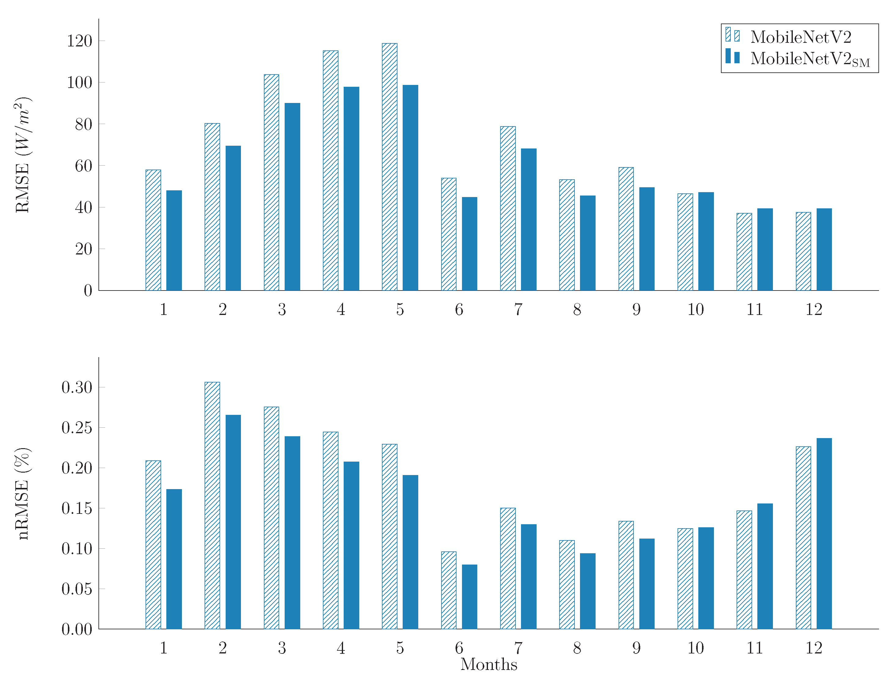
- To improve the performance of image regression CNN models, an image processing method based on sun localization is proposed which improves the accuracy of the irradiance values that the models produce, by up to 13.75% for the MobileNetV2 model.
- To showcase the applicability of the proposed method for many CNN models and for both irradiance estimation and forecasting, a study on four popular CNN models is conducted, where the method improves the results in all cases.
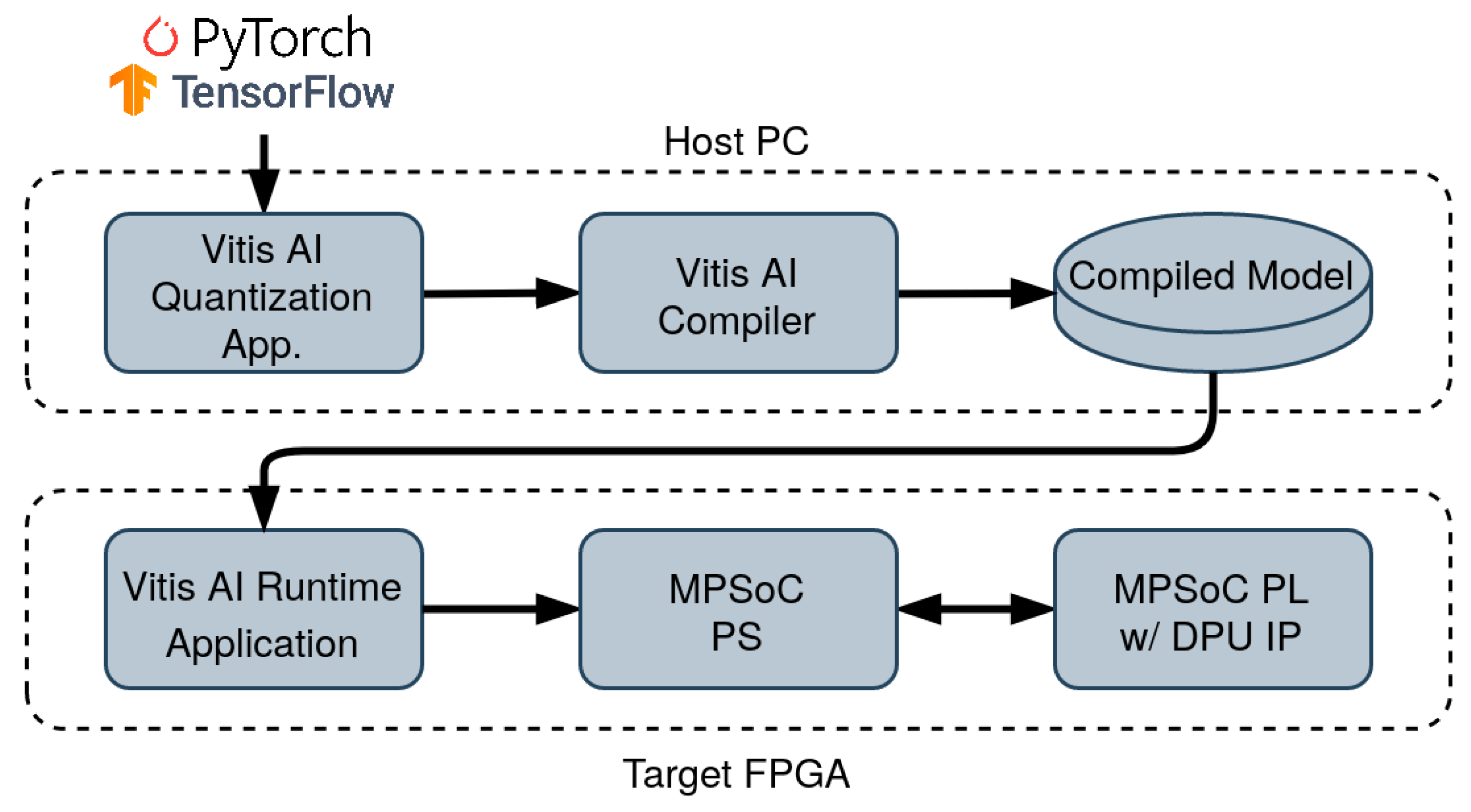
- To demonstrate the concept of a smart PV park with edge computing capabilities, we deploy the image regression CNN models on an edge FPGA using the Xilinx Vitis AI framework, achieving real-time processing rates.
2. Related Work
3. Problem Formulation & Image Dataset Analysis
3.1. Image Regression for Irradiance Forecasting Problem Formulation
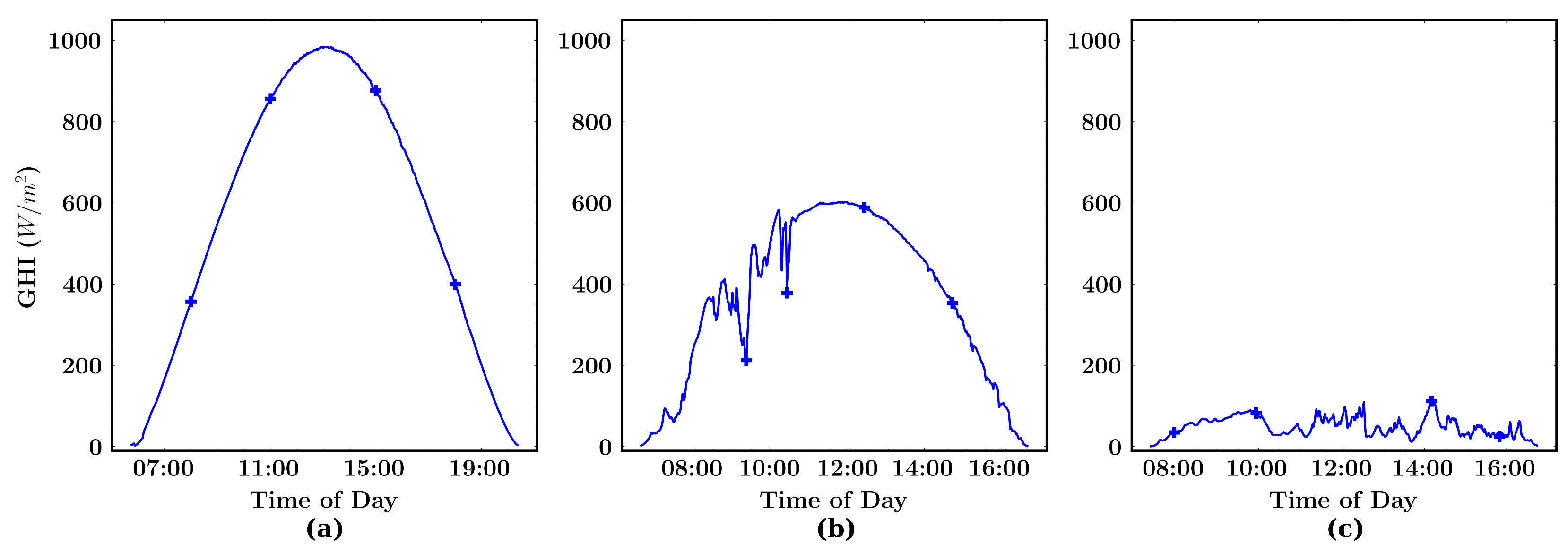
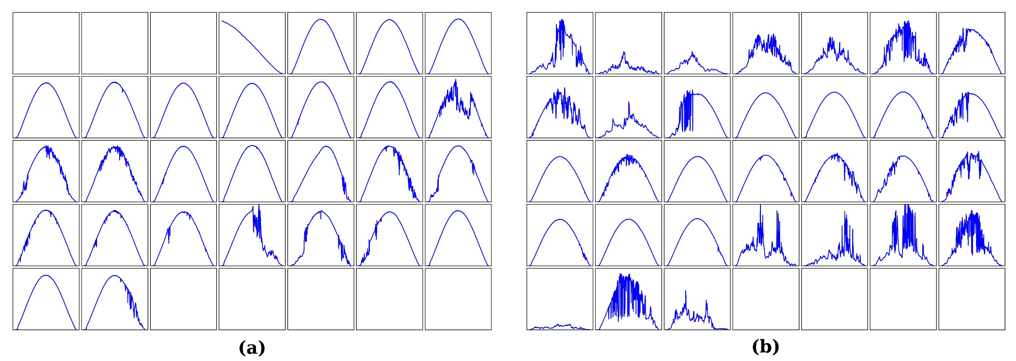
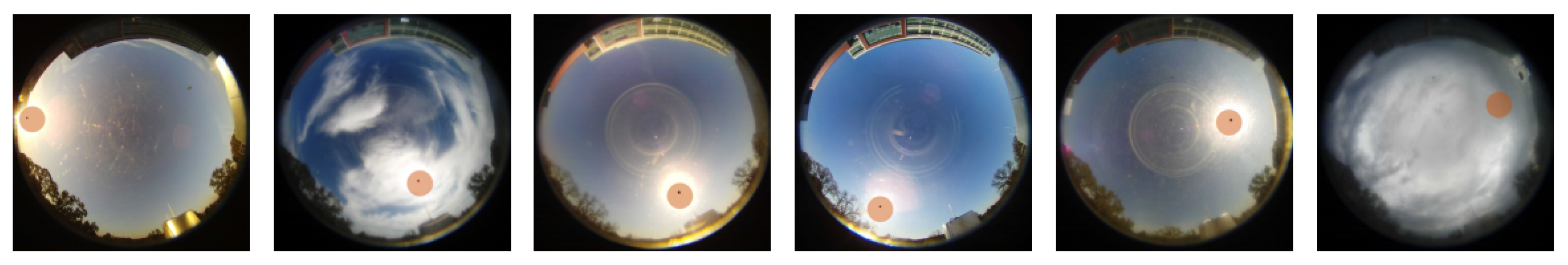
3.2. Folsom, CA Dataset Analysis
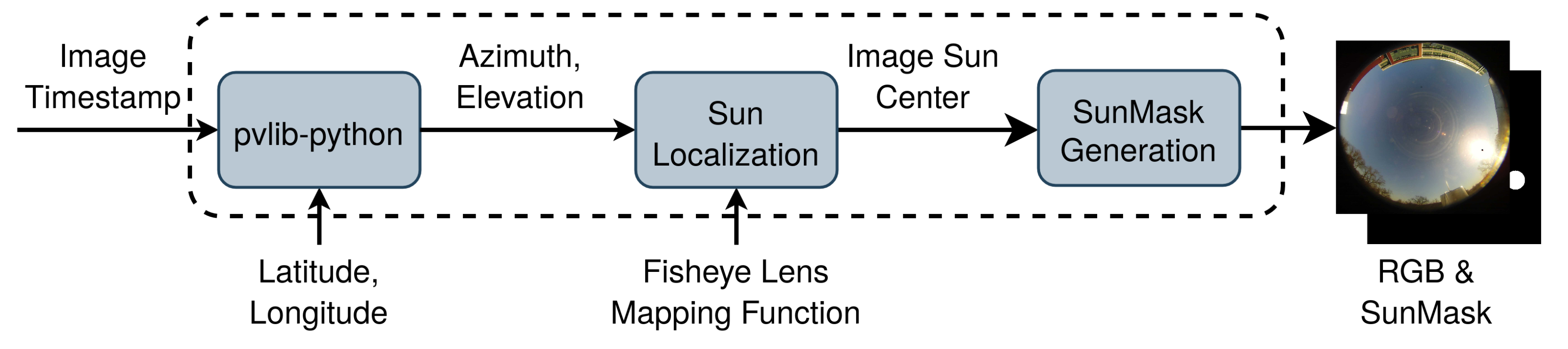
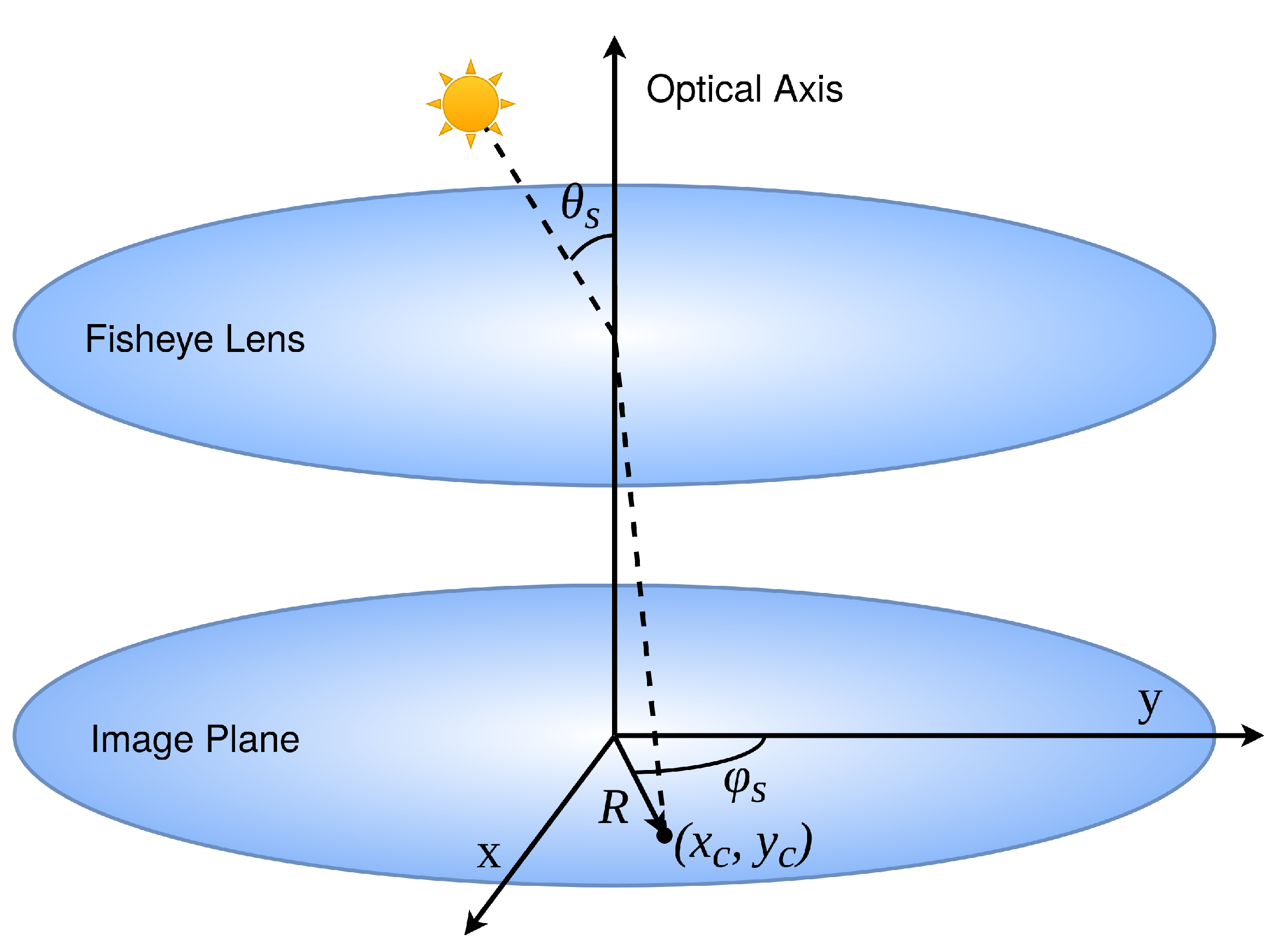
4. SunMask Generation Image Processing Method
5. Porting and Acceleration on Edge FPGA
6. Model Evaluation and Implementation Results
6.1. Image Regression Models Training and Performance Evaluation
6.2. Edge FPGA Porting and Acceleration Results
7. Conclusions
Author Contributions
Funding

Data Availability Statement
Conflicts of Interest
Abbreviations
| AI | Artificial Intelligence |
| CV | Computer Vision |
| ConvLSTM | Convolutional LSTM |
| CNN | Convolutional Neural Network |
| DL | Deep Learning |
| DPU | Deep Learning Processor Unit |
| DSP | Digital Signal Processing |
| DHI | Diffuse Horizontal Irradiance |
| DNI | Direct Normal Irradiance |
| FF | Fast Fine-tuning |
| FPGA | Field-Programmable Gate Array |
| FFs | Flip-Flops |
| FPS | Frames per Second |
| FS | Forecast Skill |
| GHI | Global Horizontal Irradiance |
| HLS | High-Level Synthesis |
| HYTA | Hybrid Thresholding Algorithm |
| IoT | Internet of Things |
| LSTM | Long Short-Term Memory |
| LUT | Lookup Table |
| ML | Machine Learning |
| MAE | Mean Absolute Error |
| MLP | Multilayer Perceptron |
| MSE | Mean Square Error |
| NRBR | Normalized Red–Blue Ratio |
| PM | Persistence Model |
| PV | Photovoltaic |
| PTQ | Post-Training Quantization |
| PS | Processing Subsystem |
| PL | Programmable Logic |
| QAT | Quantization-Aware Training |
| RBD | Red–Blue Difference |
| RBR | Red–Blue Ratio |
| RES | Renewable Energy Sources |
| RMSE | Root Mean Square Error |
| SG | Smart Grid |
| SI | Sky Imager |
| SVR | Support Vector Regression |
| SoC | System-on-Chip |
| UTC | Universal Time Coordinated |
References
- Mehmood, M.Y.; Oad, A.; Abrar, M.; Munir, H.M.; Hasan, S.F.; Muqeet, H.A.u.; Golilarz, N.A. Edge Computing for IoT-Enabled Smart Grid. Secur. Commun. Netw. 2021, 2021, 5524025. [Google Scholar] [CrossRef]
- Feng, C.; Liu, Y.; Zhang, J. A taxonomical review on recent artificial intelligence applications to PV integration into power grids. Int. J. Electr. Power Energy Syst. 2021, 132, 107176. [Google Scholar] [CrossRef]
- Zsiborács, H.; Baranyai, N.H.; Vincze, A.; Zentkó, L.; Birkner, Z.; Máté, K.; Pintér, G. Intermittent Renewable Energy Sources: The Role of Energy Storage in the European Power System of 2040. Electronics 2019, 8, 729. [Google Scholar] [CrossRef] [Green Version]
- Chen, X.; Du, Y.; Lim, E.; Fang, L.; Yan, K. Towards the applicability of solar nowcasting: A practice on predictive PV power ramp-rate control. Renew. Energy 2022, 195, 147–166. [Google Scholar] [CrossRef]
- Lin, F.; Zhang, Y.; Wang, J. Recent advances in intra-hour solar forecasting: A review of ground-based sky image methods. Int. J. Forecast. 2022. [Google Scholar] [CrossRef]
- Juncklaus Martins, B.; Cerentini, A.; Mantelli, S.L.; Loureiro Chaves, T.Z.; Moreira Branco, N.; von Wangenheim, A.; Rüther, R.; Marian Arrais, J. Systematic review of nowcasting approaches for solar energy production based upon ground-based cloud imaging. Sol. Energy Adv. 2022, 2, 100019. [Google Scholar] [CrossRef]
- Pickering, T.E. The MMT all-sky camera. In Ground-Based and Airborne Telescopes; Stepp, L.M., Ed.; International Society for Optics and Photonics, SPIE: Bellingham, WA, USA, 2006; Volume 6267, pp. 448–454. [Google Scholar] [CrossRef]
- Carreira Pedro, H.; Larson, D.; Coimbra, C. A Comprehensive Dataset for the Accelerated Development and Benchmarking of Solar Forecasting Methods; Zenodo, 2019. [Google Scholar] [CrossRef]
- Andreas, A.; Stoffel, T. REL Solar Radiation Research Laboratory (SRRL): Baseline Measurement System (BMS); NREL Report No. DA-5500-56488; NREL: Golden, CO, USA, 2019. [Google Scholar] [CrossRef]
- Véstias, M.P.; Duarte, R.P.; de Sousa, J.T.; Neto, H.C. Moving Deep Learning to the Edge. Algorithms 2020, 13, 125. [Google Scholar] [CrossRef]
- Sandler, M.; Howard, A.G.; Zhu, M.; Zhmoginov, A.; Chen, L. Inverted Residuals and Linear Bottlenecks: Mobile Networks for Classification, Detection and Segmentation. arXiv 2018, arXiv:1801.04381. [Google Scholar] [CrossRef]
- Iandola, F.N.; Moskewicz, M.W.; Ashraf, K.; Han, S.; Dally, W.J.; Keutzer, K. SqueezeNet: AlexNet-level accuracy with 50x fewer parameters and <1MB model size. arXiv 2016, arXiv:1602.073600. [Google Scholar] [CrossRef]
- Pedro, H.T.C.; Larson, D.P.; Coimbra, C.F.M. A comprehensive dataset for the accelerated development and benchmarking of solar forecasting methods. J. Renew. Sustain. Energy 2019, 11, 036102. [Google Scholar] [CrossRef] [Green Version]
- Richardson, W.; Krishnaswami, H.; Vega, R.; Cervantes, M. A Low Cost, Edge Computing, All-Sky Imager for Cloud Tracking and Intra-Hour Irradiance Forecasting. Sustainability 2017, 9, 482. [Google Scholar] [CrossRef] [Green Version]
- Miller, S.D.; Rogers, M.A.; Haynes, J.M.; Sengupta, M.; Heidinger, A.K. Short-term solar irradiance forecasting via satellite/model coupling. Sol. Energy 2018, 168, 102–117. [Google Scholar] [CrossRef]
- Ayet, A.; Tandeo, P. Nowcasting solar irradiance using an analog method and geostationary satellite images. Sol. Energy 2018, 164, 301–315. [Google Scholar] [CrossRef] [Green Version]
- Ordoñez Palacios, L.E.; Bucheli Guerrero, V.; Ordoñez, H. Machine Learning for Solar Resource Assessment Using Satellite Images. Energies 2022, 15, 3985. [Google Scholar] [CrossRef]
- Kim, B.Y.; Cha, J.W.; Chang, K.H. Twenty-four-hour cloud cover calculation using a ground-based imager with machine learning. Atmos. Meas. Tech. 2021, 14, 6695–6710. [Google Scholar] [CrossRef]
- Li, Q.; Lu, W.; Yang, J. A Hybrid Thresholding Algorithm for Cloud Detection on Ground-Based Color Images. J. Atmos. Ocean. Technol. 2011, 28, 1286–1296. [Google Scholar] [CrossRef]
- Rajagukguk, R.A.; Kamil, R.; Lee, H.J. A Deep Learning Model to Forecast Solar Irradiance Using a Sky Camera. Appl. Sci. 2021, 11, 5049. [Google Scholar] [CrossRef]
- Zuo, H.M.; Qiu, J.; Jia, Y.H.; Wang, Q.; Li, F.F. Ten-minute prediction of solar irradiance based on cloud detection and a long short-term memory (LSTM) model. Energy Rep. 2022, 8, 5146–5157. [Google Scholar] [CrossRef]
- Chu, Y.; Li, M.; Coimbra, C.F. Sun-tracking imaging system for intra-hour DNI forecasts. Renew. Energy 2016, 96, 792–799. [Google Scholar] [CrossRef]
- Niccolai, A.; Nespoli, A. Sun Position Identification in Sky Images for Nowcasting Application. Forecasting 2020, 2, 488–504. [Google Scholar] [CrossRef]
- Paletta, Q.; Lasenby, J. A Temporally Consistent Image-based Sun Tracking Algorithm for Solar Energy Forecasting Applications. In Proceedings of the NeurIPS 2020 Workshop on Tackling Climate Change with Machine Learning, Virtual, 11–12 December 2020. [Google Scholar]
- Paletta, Q.; Arbod, G.; Lasenby, J. Benchmarking of deep learning irradiance forecasting models from sky images—An in-depth analysis. Sol. Energy 2021, 224, 855–867. [Google Scholar] [CrossRef]
- Wen, H.; Du, Y.; Chen, X.; Lim, E.; Wen, H.; Jiang, L.; Xiang, W. Deep Learning Based Multistep Solar Forecasting for PV Ramp-Rate Control Using Sky Images. IEEE Trans. Ind. Inform. 2021, 17, 1397–1406. [Google Scholar] [CrossRef]
- Jiang, H.; Gu, Y.; Xie, Y.; Yang, R.; Zhang, Y. Solar Irradiance Capturing in Cloudy Sky Days–A Convolutional Neural Network Based Image Regression Approach. IEEE Access 2020, 8, 22235–22248. [Google Scholar] [CrossRef]
- Wang, F.; Zhang, Z.; Chai, H.; Yu, Y.; Lu, X.; Wang, T.; Lin, Y. Deep Learning Based Irradiance Mapping Model for Solar PV Power Forecasting Using Sky Image. In Proceedings of the 2019 IEEE Industry Applications Society Annual Meeting, Baltimore, MD, USA, 29 September–3 October 2019; pp. 1–9. [Google Scholar] [CrossRef]
- Song, S.; Yang, Z.; Goh, H.; Huang, Q.; Li, G. A novel sky image-based solar irradiance nowcasting model with convolutional block attention mechanism. Energy Rep. 2022, 8, 125–132. [Google Scholar] [CrossRef]
- Paletta, Q.; Hu, A.; Arbod, G.; Lasenby, J. ECLIPSE: Envisioning CLoud Induced Perturbations in Solar Energy. Appl. Energy 2022, 326, 119924. [Google Scholar] [CrossRef]
- Tran, Q.K.; Song, S.k. Computer Vision in Precipitation Nowcasting: Applying Image Quality Assessment Metrics for Training Deep Neural Networks. Atmosphere 2019, 10, 244. [Google Scholar] [CrossRef]
- Le Guen, V.; Thome, N. A Deep Physical Model for Solar Irradiance Forecasting with Fisheye Images. In Proceedings of the 2020 IEEE/CVF Conference on Computer Vision and Pattern Recognition Workshops (CVPRW), Seattle, WA, USA, 14–19 June 2020; pp. 2685–2688. [Google Scholar] [CrossRef]
- Holmgren, W.F.; Hansen, C.W.; Mikofski, M.A. pvlib python: A python package for modeling solar energy systems. J. Open Source Softw. 2018, 3, 884. [Google Scholar] [CrossRef] [Green Version]
- Xilinx. Zynq UltraScale+ MPSoC. Available online: https://www.xilinx.com/products/silicon-devices/soc/zynq-ultrascale-mpsoc.html (accessed on 15 October 2022).
- Xilinx. Please Confirm if This Author Name Is Correct? Vitis AI User Guide UG1414 (v2.5). 2022. Available online: https://docs.xilinx.com/r/en-US/ug1414-vitis-ai (accessed on 15 October 2022).
- Nagel, M.; Baalen, M.V.; Blankevoort, T.; Welling, M. Data-Free Quantization through Weight Equalization and Bias Correction. In Proceedings of the 2019 IEEE/CVF International Conference on Computer Vision (ICCV), Seoul, Republic of Korea, 27 October–2 November 2019; pp. 1325–1334. [Google Scholar] [CrossRef] [Green Version]
- Hubara, I.; Nahshan, Y.; Hanani, Y.; Banner, R.; Soudry, D. Improving Post Training Neural Quantization: Layer-wise Calibration and Integer Programming. arXiv 2020, arXiv:2006.10518. [Google Scholar] [CrossRef]
- Simonyan, K.; Zisserman, A. Very Deep Convolutional Networks for Large-Scale Image Recognition. arXiv 2014, arXiv:1409.1556. [Google Scholar] [CrossRef]
- He, K.; Zhang, X.; Ren, S.; Sun, J. Deep Residual Learning for Image Recognition. arXiv 2015, arXiv:1512.03385. [Google Scholar] [CrossRef]
- Naushad, R.; Kaur, T.; Ghaderpour, E. Deep Transfer Learning for Land Use and Land Cover Classification: A Comparative Study. Sensors 2021, 21, 8083. [Google Scholar] [CrossRef] [PubMed]


| Model | # Parameters | # OPs (Mult-Adds) |
|---|---|---|
| VGG11 | 128.77 Mil. | 2.57 G |
| ResNet-50 | 23.51 Mil. | 1.33 G |
| MobileNetV2 | 2.23 Mil. | 0.10 G |
| SqueezeNet | 0.74 Mil. | 0.23 G |
| Model | RMSE (W/m) | nRMSE (%) | MAE (W/m) |
|---|---|---|---|
| VGG11 | 65.25 | 15.88 | 38.31 |
| VGG11SM | 59.03 | 14.36 | 32.93 |
| ResNet-50 | 64.83 | 15.77 | 37.23 |
| ResNet-50SM | 60.31 | 14.67 | 36.02 |
| MobileNetV2 | 75.95 | 18.48 | 47.74 |
| MobileNetV2SM | 65.51 | 15.94 | 39.53 |
| SqueezeNet | 70.18 | 17.08 | 44.65 |
| SqueezeNetSM | 62.93 | 15.31 | 38.56 |
| Horizon | Model | RMSE (W/m) | nRMSE (%) | FS (%) |
|---|---|---|---|---|
| Persistence | 72.64 | 17.32 | - | |
| 5-min | Resnet-50 | 73.18 | 17.44 | −0.75 |
| Resnet-50SSM | 66.79 | 15.93 | 8.04 | |
| Persistence | 86.77 | 20.26 | - | |
| 10-min | Resnet-50 | 78.06 | 18.23 | 10.04 |
| Resnet-50SSM | 73.06 | 17.06 | 15.80 | |
| Persistence | 94.52 | 21.67 | - | |
| 15-min | Resnet-50 | 80.87 | 18.54 | 14.44 |
| Resnet-50SSM | 75.78 | 17.37 | 19.83 |
| Model | Quantization Method | RMSE (W/m) | nRMSE (%) | MAE (W/m) |
|---|---|---|---|---|
| VGG11 | PTQ | 176.48 | 42.94 | 38.31 |
| PTQ & FF | 69.51 | 16.91 | 41.04 | |
| ResNet-50 | PTQ | 68.37 | 16.63 | 40.39 |
| PTQ & FF | 67.01 | 16.30 | 39.18 | |
| MobileNetV2 | PTQ | 88.42 | 21.51 | 59.91 |
| PTQ & FF | 88.78 | 21.60 | 60.67 | |
| SqueezeNet | PTQ | 89.94 | 21.89 | 63.24 |
| PTQ & FF | 77.02 | 18.74 | 50.30 | |
| PTQ & QAT | 72.27 | 17.58 | 45.84 |
| Resource | 2-Core DPU IP | 1-Core DPU IP |
|---|---|---|
| LUTs | 108K (47%) | 50K (22%) |
| FFs | 204K (44%) | 98K (21%) |
| DSPs | 1394 (81%) | 690 (40%) |
| RAMBs | 203 (65%) | 145 (46%) |
Publisher’s Note: MDPI stays neutral with regard to jurisdictional claims in published maps and institutional affiliations. |
© 2022 by the authors. Licensee MDPI, Basel, Switzerland. This article is an open access article distributed under the terms and conditions of the Creative Commons Attribution (CC BY) license (https://creativecommons.org/licenses/by/4.0/).
Share and Cite
Papatheofanous, E.A.; Kalekis, V.; Venitourakis, G.; Tziolos, F.; Reisis, D. Deep Learning-Based Image Regression for Short-Term Solar Irradiance Forecasting on the Edge. Electronics 2022, 11, 3794. https://doi.org/10.3390/electronics11223794
Papatheofanous EA, Kalekis V, Venitourakis G, Tziolos F, Reisis D. Deep Learning-Based Image Regression for Short-Term Solar Irradiance Forecasting on the Edge. Electronics. 2022; 11(22):3794. https://doi.org/10.3390/electronics11223794
Chicago/Turabian StylePapatheofanous, Elissaios Alexios, Vasileios Kalekis, Georgios Venitourakis, Filippos Tziolos, and Dionysios Reisis. 2022. "Deep Learning-Based Image Regression for Short-Term Solar Irradiance Forecasting on the Edge" Electronics 11, no. 22: 3794. https://doi.org/10.3390/electronics11223794
APA StylePapatheofanous, E. A., Kalekis, V., Venitourakis, G., Tziolos, F., & Reisis, D. (2022). Deep Learning-Based Image Regression for Short-Term Solar Irradiance Forecasting on the Edge. Electronics, 11(22), 3794. https://doi.org/10.3390/electronics11223794