Inverse Dynamics Modeling and Analysis of Healthy Human Data for Lower Limb Rehabilitation Robots

Abstract

Bio-controllers inspired by the characteristics of the human lower limb play an important role in the study of lower limb rehabilitation robots (LLRRs). However, the inverse dynamics modeling of robots for human lower limb rehabilitation remains a challenging issue due to the non-linear and strong coupling characteristics of the bio-controller. To further improve the inverse dynamics model’s accuracy, this paper proposes the use of a non-parametric modeling approach in order to learn it. In detail, the main idea is to use the motion data of the main joints of the lower limbs of healthy people as an input and the corresponding joint moments as an output, which are learned through the training of a neural network. To ensure that the learned model can be used on LLRRs, all data collected in this paper are real data from human lower limbs. In addition, since the type of data collected is time series, this paper proposes the use of the long short-term memory (LSTM) and gated recurrent unit (GRU) networks to learn the inverse dynamics model of the robot-like human lower limb and to compare the learning effects of the two networks. The evaluation metric for both network models is the root mean square error (RMSE). The experimental results show that both networks have sound learning effects, and that the GRU network has a more significant learning ability than the LSTM network.

1. Introduction

In recent years, there has been an increasing number of hemiplegic patients due to stroke or paraplegic patients due to spinal cord injury [1,2], accompanied by the intensification of global population aging. Lower limb rehabilitation robots (LLRRs) (Figure 1) can help patients to gradually regain their ability to walk, and are currently a hot topic in the medical robotics research field [3]. The LLRR is Fourier X2, which has two degrees of freedom in the sagittal plane for the hip and knee joints. Some rehabilitation robots have been studied with some progress, such as LOPES [4], ALEX [5], WalkTrainer [6], Lokomat [7], and MINDWALKER [8], which have been tested and verified to assist sufferers in recovering their exercise ability by allowing patients to effectively complete repetitive activities [9,10].

Using inverse dynamics modeling on LLRR to achieve a high control accuracy is still a challenging issue. The learning problem of the inverse dynamics model based on the inspiration of the dynamics of the human lower limb requires further investigation. The robot’s inverse dynamics problem entails that the robot’s motion state at each instant (joint angle, angular velocity, angular acceleration, etc.) is known, and that the joint torque required by the robot at the corresponding moment should be obtained. In fact, many aspects of a robot may be affected by inaccurate inverse dynamics models. For example, in the process of a human–computer interaction, accurate robot dynamics are required to achieve the tracking control of the target trajectory [11]. In torque control, precise torque is required to efficiently drive the joints of the LLRRs [12]. A slight error will not only fail to achieve a good rehabilitation effect but is also extremely likely to cause secondary injury to patients. Therefore, accurate inverse dynamics models are essential for the investigation of the motion control of LLRRs.

Currently, there are three main types of inverse dynamics learning methods: parametric [13,14,15,16], non-parametric [17,18,19,20,21,22], and semi-parametric [23,24]. Here, whether the inverse dynamic model is parameterized depends on whether the physical parameters of the robot are used. The parametric-based model usually uses the classical rigid body kinematics equation to model the robot. For example, the Lagrangian equations and the Newton–Euler are two commonly parametric methods [13,14]. These two methods solve the physical parameters via recursion, and the derivation process involves a detailed understanding of the physical properties of the robots and expresses them in mathematical formulas. As a result, solving these equations usually takes time, and the resultant LLRRs generally run at a low speed, which will cause jitter and other situations during their run-time. To improve the model’s accuracy, it is also required to identify the derived model so that a more accurate model can be developed. In summary, the parametric modeling approaches need to deal with uncertainties [15,16], such as friction, non-linearity, and noise, which cannot be modeled in a parametric way but lead to significant inaccuracies in the model.

On the other hand, the non-parametric models solve inverse dynamics using machine learning methods, which learn the physical parameters directly from data. This method allows the model to learn any nonlinear structures, including friction, noise, and other uncertainties in parametric models. For example, the inverse dynamics model of a manipulator is learned using a recurrent neural network (RNN) in [17]. The inverse dynamics model is learned using an O(n)-based LSTM network in [18], and it is assessed on a KUKA robot arm. The hierarchical recurrent network is used to learn the manipulator’s inverse dynamics model in [19]. The above three methods [17,18,19] are datasets or data collected from the sensors of the robot. In addition, their application objects are robotic arms. The data used in this paper are real human data, and the application objects are LLRRs. In addition to studies based on non-parametric inverse dynamics models, other studies on predicting lower limb joint moments from LLRRs have been conducted in recent years. For example, in [20], it is based on the LSTM neural network and transfers learning to predict the joint torque of the lower limbs of the human body. The data are derived from the electromyography (EMG) signals and joint angles of the lower limbs of the human body, and each time step’s data contain thirteen EMG signals and four joint angles. However, the EMG signals can be affected by the secretions on the skin surface or the offset of the sensor position, which can affect the accuracy of EMG signals acquisition. In [21], four types of neural networks are utilized to predict ankle joint torque and the learning effects of the four types of regression models are compared. The data come from the EMG signals and accelerometer data of the lower limbs of the human body, but only the torque prediction of the ankle joint is made. In [22], the predictive ability of mechanomyography (MMG) and EMG for assist-as-needed lower-limb-exoskeleton-controlled human knee torque was compared by various interaction conditions. In [20,21,22], both the combination of EMG signals and other signals are used to predict the joint moments of human lower limbs, but the data used are not the joint angles, angular velocities, and angular accelerations of human lower limbs. In a physical sense, there is no interpretability and it can only be considered a black box model, and so cannot be considered as a method of learning the inverse dynamics model. However, the method of the non-parametric model also has its limitations: if the data are of poor quality or limited in quantity, this can affect the accuracy of the model.

The semi-parametric model combines the parametric model and the non-parametric model. Generally, the parameterizable design deals with the traditional inverse dynamics of the rigid body, and the non-parametric part is used for the nonlinear error that cannot be accurately defined by the parametric part [23]. However, the semi-parametric model’s learning process is biased towards the parametric component, which reduces the contribution of the non-parametric component [24]. In addition, the semi-parametric model incorporates many more computational steps than the other two methods, since not only parametric but also non-parametric models need to be built.

To avoid the drawback of using non-parametric methods to estimate the inverse dynamics, which will be further applied in LLRR, the data in this paper were obtained from the motion data of the major joints of the lower extremities in healthy individuals. Because the purpose of lower extremity rehabilitation is mainly to enable patients with lower extremity motor dysfunction to walk like healthy people [25], this set of gait data obtained from healthy people will guarantee the LLRR bio-inspired controller to work as the desired human gait trajectory so that the humanoid motion of the LLRR can be realized and, in turn, a good rehabilitation effect can be achieved [26]. Specifically, the collected angles, angular velocity, and angular acceleration of each joint of the lower limbs of the human body that can be used for LLRRs were input into the trained model to predict the torque of the joints corresponding to LLRRs. More importantly, in terms of generalizability, we can predict the required motion trajectory of the patient from the physical parameters of the patient’s body (height, weight, stride length, thigh and calf length, etc.) and then predict the joint moments by the method proposed in this paper [27,28]. In addition, the mapping relationship between the motion data of each joint of the human lower limb and the moment data of the corresponding joint is also crucial for the study of the LLRRs controller [29].

To address the aforementioned problems, an inverse dynamic model of the human lower limb using LLRRs based on variants of RNNs is proposed in this paper. Considering that the data in this article were directly derived from the three-dimensional optical motion capture system and three-dimensional force measuring platform, the data quality can be ensured. In addition, the number of available data that we collected was 27,608, which is large enough. Therefore, we adopted a non-parametric learning method to learn the inverse dynamics model.

This article’s main contributions are threefold:

• This paper proposes the use of a non-parametric modeling approach (long short-term memory (LSTM) and gated recurrent unit (GRU) network) to learn the inverse dynamics model of a robot-like human lower limb.
• Comparing the learning effects of the two neural networks, we can obtain that, under the same number of iterations, the GRU network requires a shorter training time than the LSTM network, and the learned model works better.
• The motion data of the lower limbs of a healthy person were captured by a 3D motion capture system, and the captured data were processed to obtain data that can be used for model learning.

The structure of the remainder of the paper is described below. Section 2 focuses on the research framework and the formulaic definition of the research question. Section 3 is the research methodology and confirmed effectiveness. Here, first, the experimental subject and the collection and processing of data are described. Second, the basic concepts of the two network learning models and the proposed learning model framework are introduced. Finally, the empirical results are presented. Section 4 mainly discusses the research of this paper and gives the future development direction of the experiment.

2. Methodology

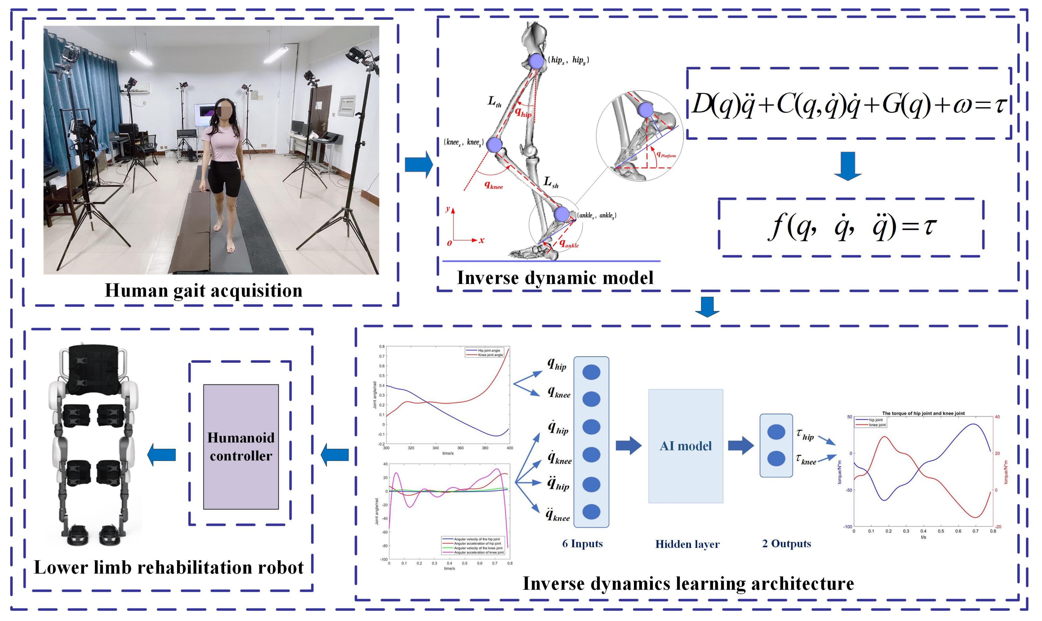
2.1. Framework

The overall framework of this model is shown in Figure 2. Firstly, gait and plantar force data sets were collected from a healthy person during normal walking of the lower limbs using a 3D motion capture system and a 3D force measuring platform. Then, an inverse dynamics model of the human body was built for LLRRs. Next, the collected data were processed, and their model was learned through the established inverse dynamics model learning architecture. Finally, the derived model could then be applied to the bio-controller of LLRRs.

2.2. Problem Formulation

In this section, we will analyze the problem of learning the inverse dynamic model of the human lower limb during normal walking. According to [30,31], a traditional parametric model of inverse dynamics can be deduced. Typically, the inverse dynamics equation for the lower limb can be represented as:

$$\begin{array}{c}\hfill D\left(q\right)\ddot{q}+C(q,\dot{q})\dot{q}+G\left(q\right)+\omega =\tau \end{array}$$

(1)

where q, $\dot{q}$ and $\ddot{q}$, respectively, denote the joint angle, joint angular velocity, and joint angular acceleration of each joint of the human lower limbs that can be used for LLRRs. $\tau$ represents the joint torque. $D\left(q\right)\in R^{2\times 2}$ represents the inertia matrix of positive definite. $C(q,\dot{q})\in R^{2\times 2}$ is the matrix of the force of Coriolis and centrifugal force. $G\left(q\right)\in R^{2\times 1}$ is the gravity matrix. $\omega$ is various errors and perturbations.

The main objective of this paper is to solve the inverse dynamic model (Equation (1)) without explicitly including the physical parameters. Given three input vectors q, $\dot{q}$, $\ddot{q}$ and an output vector $\tau$, the target learning function is:

$$f(q,\dot{q},\ddot{q})=\tau$$

(2)

We will solve the problem through a data-driven method. This approach can not only eliminate the errors induced by the terms that cannot be modeled by the traditional parametric model but also saves efforts by avoiding the tedious derivation of mathematical formulae in the modeling process.

2.3. Inverse Dynamics Model Learning

The data-driven method is realized by neural network learning. In this section, we will first introduce two learning methods, namely long short-term memory (LSTM) and gated recurrent unit (GRU), for inverse dynamics modeling of the lower limb. Since LSTM and GRU networks are variants of RNNs, they are both proposed to handle temporal sequence problems. The signals obtained from gait classification [32,33], motion prediction [34,35], and learning dynamics models [36,37] are temporal sequences that have been widely applied in RNN methods. Therefore, in this paper, both networks were used to learn the inverse dynamics model, and the learning effects of the two networks were compared. The third section presents the proposed learning architecture for the bio-controller of LLRRs.

2.3.1. Long Short Term Memory

Hochreiter and Schmidhuber (1997) proposed LSTM as a specific form of a RNN [38]. In the traditional RNN model, there are no memory cells. Therefore, if the sequence is too long, it tends to lead to vanishing gradient or exploding gradient problems. On the other hand, LSTM networks have memory cells that selectively remember important information and filter other useless information, reducing their memory burden and speeding up the training of the model. There are three gating units in the LSTM network that play a role in the overall network: from highest to lowest, forget gate $f_t$, input gate $i_t$, and output gate $o_t$. Figure 3 depicts the gates in an LSTM network, and Equations (3)–(7) illustrate how to calculate it.

$$f_t=\sigma \left(W_f{x}_t+U_f{h}_{t-1}+b_f\right)$$

(3)

$$i_t=\sigma \left(W_i{x}_t+U_i{h}_{t-1}+b_i\right)$$

(4)

$$o_t=\sigma \left(W_o{x}_t+U_o{h}_{t-1}+b_0\right)$$

(5)

$$c_t=f_t\odot c_{t-1}+i_t\odot tanh\left(W_c{x}_t+U_c{h}_{t-1}+b_c\right)$$

(6)

$$h_{t}a=o_t\odot tanh\left(c_t\right)$$

(7)

2.3.2. Gated Recurrent Unit

Cho (2014) proposed the GRU network [39]. The GRU network is an improvement on the LSTM network because it has a more straightforward structure. The GRU network has only two gates: the update gate $z_t$, and the reset gate $r_t$, respectively. In addition, GRU networks reduce the risk of over-fitting [40]. Similar to LSTM, the reset gate is used to adjust the degree to which the state information from the previous instant and the current moment are combined. The larger the reset gate value, the greater the degree of combination. Compared with the LSTM network, the simplified GRU network reduces the training parameters, reduces the learning time requirement, and predicts better than the LSTM network in most of the predictions [41]. Figure 4 depicts the GRU architecture, and Equations (8)–(11) illustrate how to calculate it.

$$z_t=\sigma \left(W_z{x}_t+U_z{h}_{t-1}+b_z\right)$$

(8)

$$r_t=\sigma \left(W_r{x}_t+U_r{h}_{t-1}+b_r\right)$$

(9)

$${\tilde{h}}_t=tanh\left(W_{\tilde{h}}{x}_t+U_{\tilde{h}}\left(r_t\otimes h_{t-1}\right)+b_{\tilde{h}}\right)$$

(10)

$$h_t=\left(1-z_t\right)\otimes h_{t-1}+z_t\otimes {\tilde{h}}_t$$

(11)

The weight matrices for the two networks above are denoted by W and U. The related bias vector is denoted by b. The sigmoid activation function is represented by $\sigma$. The hyperbolic tangent activation function is denoted by the symbol ‘tanh’.

2.3.3. Proposed Learning Architecture

The LSTM or GRU was then plugged into the predictive architecture as shown in Figure 5, with five layers, including an input layer, a hidden layer, a loss layer, a fully connected layer, and a regression output layer.

The joint angles, joint angular velocity, and joint angular acceleration of the human hip and knee joints were entered into the input layer. Each joint has three parameters, and there are six parameters in total; see Figure 6. The input parameters were then processed for outliers, normalized, and adjusted before being sent into the neural network’s hidden layer. The output layer is the moment where we want to predict the hip and knee joints of the human lower limbs.

A network model was normalized to improve the accuracy and to speed up the convergence to speed up the training. The input data’s maximum and minimum values were limited to stay within the hidden layer function and output layer function’s bounds. This approach (Equation (12)) is commonly used in machine learning:

$$\widetilde{x_i}=\frac{x_i-x_{min}}{x_{max}-x_{min}}i=1,2,\cdots ,n$$

(12)

where $x_{min}$ and $x_{max}$ are the minimum and maximum values of $x_i$, respectively. ‘Tanh’ is the state activation function of the network cell (Equation (13)). ‘Sigmoid’ is the gate activation function (Equation (14)). ‘Glorot’ is used as the initial value to initialize the input weights. The recurrent weights initializer was set with orthogonal as the initial value, and the bias with zeros was initialized. It is defined as follows.

Hyperbolic tangent activation function:

$$tanh\left(x\right)=\frac{e^x-e^{-x}}{e^x+e^{-x}}$$

(13)

Sigmoid activation function:

$$\sigma \left(x\right)=\frac{1}{1+e^x}$$

(14)

To avoid overfitting, the dropout layer was set to 0.2 [42]. The regression output layer was immediately linked by the fully connected layer. The dropout layer used ‘glorot’ as the initial value to initialize the input weight. Zeros were used to initialize the bias. Joint moments are required for the output of LLRRs in the regression layer. The root mean square error (RMSE) was used as an evaluation metric to determine the predictive performance of robot-like human lower limb inverse dynamics. The smaller the RMSE value, the better the prediction performance of the model. It is defined as follows:

$$RMSE=\sqrt{\frac{1}{N}\sum _{i=1}^N{\left(p_i-y_i\right)}^2}$$

(15)

where $p_i$ and $y_i$ are the $i-th$ anticipated and actual values, respectively, and N denotes the total number of data points.

3. Experiment

3.1. Experimental Subject

The research subject of this paper was a healthy woman with a height of 168 cm, an age of 25, and a weight of 52 kg, who had no history of nerve damage or muscle disease. The experimental protocol was approved by the Ethics Committee of Zhongyuan Institute of Technology, Zhengzhou City, Henan Province, and informed consent was obtained from the participants.

3.2. Data Collection

The gait data were obtained from the NOKOV 3D optical motion capture system (Figure 7), which consists of six infrared cameras sampling at 120 Hz. The infrared cameras capturing three-dimensional data of human lower limb movements were collected by eight reflex marker points, which were affixed to the main joints of the subject’s lower limbs. Marker focuses were put by the Helen Hayes placement protocol (Figure 8) [43]. At the same time, we acquired the 3D plantar force data of a healthy person through 4 Bertec 3D force measurement platforms (Figure 7), and the sampling frequency was 120 Hz. The 3D plantar force data were acquired simultaneously to keep the data synchronized with the motion capture system, which was convenient for subsequent data processing.

In the experimental stage, the subject naturally swung her hands and looked at the markers on the wall to ensure a natural gait when walking. To ensure the accuracy of the plantar force collection during walking, the tester was required to measure barefoot so that the plantar could be in full contact with the force measuring platform.

The subject was asked to constantly and naturally walk around the data collection site, eventually screening the data for 70 gait cycles. Due to the symmetry of the two legs, all data from the subject’s right leg during these 70 cycles were selected for this paper. After a series of data processing, 3451 time series of data were obtained. There were 8 joint data (hip and knee joint angles, angular velocities, angular accelerations, joint moments) per time series, and a total of 27,608 data were utilized to learn the robot-like of human lower limb inverse dynamics model.

Table 1. Details of the datasets.

Input Value	Data Bulk	Target Value	Data Bulk
Hip joint angle	3451	Moment of hip joint	3451
Hip joint angular velocity	3451
Angular acceleration of hip joint	3451
Knee joint angle	3451	Moment of knee joint	3451
Knee joint angular velocity	3451
Angular acceleration of Knee joint	3451

presents the real-world motion data sets for hip and knee joint angles, angular velocities, angular accelerations, and joint moments for the subject’s lower extremities. There are 3451 data points for each joint.

Since most LLRRs only support movement in the sagittal plane, the motion trajectories of the human lower extremity joints in this paper are expressed as: flexion and extension of the hip, and flexion and extension of the knee in the sagittal plane.

3.3. Preprocessing of Collected Data

Whether the gait data acquired are good or not will directly affect the learning effectiveness of the robot-like inverse dynamics model of human lower limb. The original gait data of the major joints of the lower limbs and the original plantar force data collected from the 3D motion collection system must be further processed in order to generate good training data and accelerate the training of the neural network.

• Filtering and fitting:
  To reduce the noise disturbance of the raw signal, we must filter the data using the acquisition system’s software Seeker. If the data frame is lost during processing, the cubic spline difference needs to be performed to ensure the accuracy of the data. If the data frame is lost too much, this set of data is directly discarded.
• Removing invalid data:
  Data can be lost or misplaced if the marker point is obscured by a swinging arm or if the foot is off the force measuring platform when collecting data. Additionally, there are four force plates, with a space between each couple. If the subject walks between the force plates, the gait data and plantar force data acquired will be erroneous, particularly the sole force data. Therefore, not all gait and plantar force data are valid and we need to delete these invalid data and remove them manually.
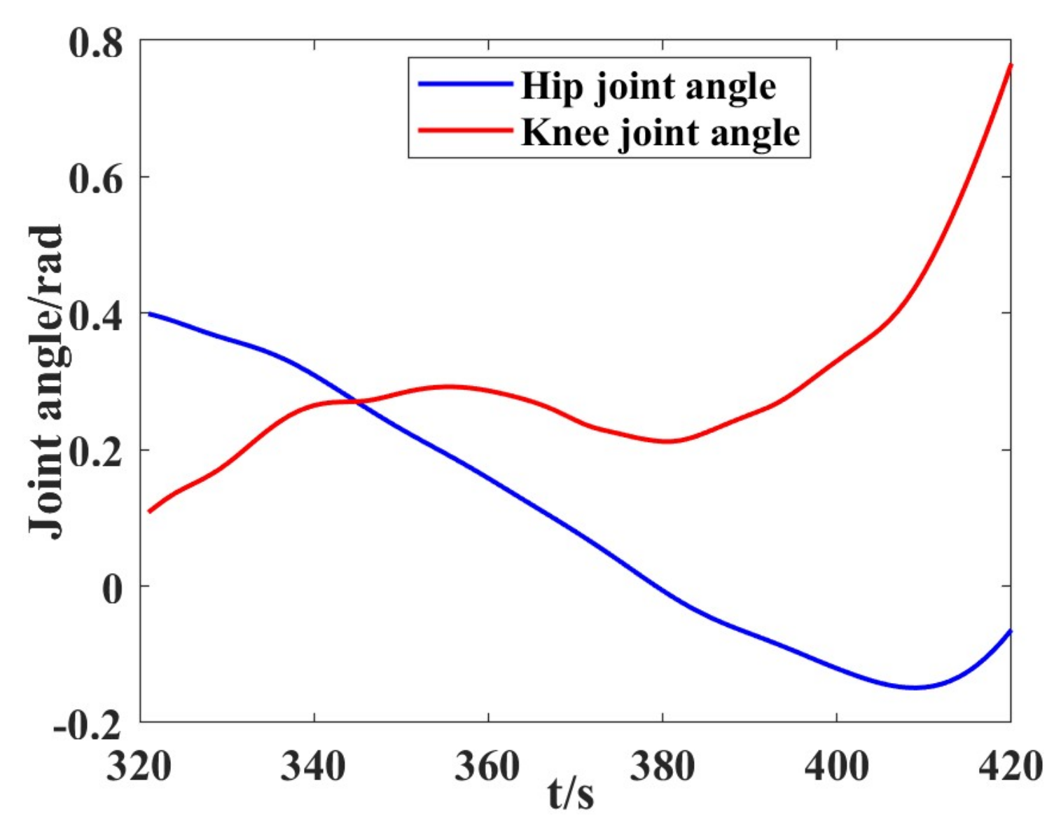
• Data processing of human lower limb joint angles, angular velocities, and angular accelerations:
  In this paper, an inverse dynamics analysis was used to model the human lower limb as a two-linked rod (Figure 9) using data on the position of the ends of individual joints at different moments in time, captured by a 3D motion capture system during human movement. Equations (16) and (17) calculate the joint angles of the hip and knee at different moments (Figure 10). To ensure that the derived trajectory data can be used directly in LLRRs, the derived joint angles were fitted by Fourier function curves (Equation (18)). The fitted Fourier function was derived to obtain the joint angular velocities of the hip and knee joints, and the quadratic derivative was used to acquire the corresponding accelerations (Figure 11).
• Human gait force data processing:
  The force data $f_{\mathrm{x}}$ and $f_{\mathrm{y}}$ of the joint end position of the subject’s lower limb were measured by the 3D force measurement platform. The moment components $M_x$ and $M_y$ of the two joints end positions were calculated (Equation (19)). Finally, the two joint moments (Figure 12) were derived from the Jacobian matrix (Equation (20)).

$$q_{hip}=arctan\frac{kne{e}_x-{hip}_x}{{knee}_y-hi{p}_y}$$

(16)

$$q_{knee}=q_{hip}-arctan\frac{{ankle}_x-{knee}_x}{{ankle}_y-{knee}_y}$$

(17)

$$f\left(x\right)=a_0+\sum _{i=1}^n\left\{a_{i}cos\left(wx\right)+b_{i}sin\left(wx\right)\right\}$$

(18)

$$M_x=f_{\mathrm{x}}\left({ankle}_y-hi{p}_y\right),M_y=f_y\left({ankle}_x-hi{p}_x\right)$$

(19)

$$\left[\begin{array}{c}{\tau }_{\mathrm{hip}}\\ {\tau }_{\mathrm{knee}}\end{array}\right]={\left[\begin{array}{cc}{L}_{rh}cos{q}_{hip}+L_{sh}cos\left(q_{hip}-q_{\mathrm{knee}}\right)& -L_{sh}cos\left(q_{hip}-q_{\mathrm{knee}}\right)\\ -L_{rh}sin{q}_{hip}-L_{sh}sin\left(q_{\mathrm{hip}}-q_{\mathrm{knee}}\right)& L_{sh}sin\left(q_{hip}-q_{\mathrm{knee}}\right)\end{array}\right]}^{\mathrm{T}}\left[\begin{array}{c}{M}_x\\ M_y\end{array}\right]$$

(20)

3.4. Experimental Results

In this paper, we processed data and learned the inverse dynamics model on a laptop using MATLAB R2022a. The experiment first divided the training and test sets into 9:1 and then divided the training and test sets into 8:2 under the same conditions. “MaxEpochs” was set to 100. “GradientThreshold” was set to 1. “InitialLearnRate” was set to 0.005. “LearnRateDropPeriod” was set to 100. “LearnRateDropFactor” was set to 0.8. “ValidationFrequency” was set to 5. Comparing the experimental results by changing the number of iterations several times, it was found that the two networks with neither over-fitting nor under-fitting had the smallest and most stable values of the loss function at nearly 100 iterations. The comparative results of the data trained by this model are shown in

Table 2. Comparison of the RMSE of several RNN versions.

	Train Ratio	Method	Epoch	Time (s)	RMSE
27,608 samples	0.9	LSTM	100	3.12 s	0.19334
		GRU	100	1.54 s	0.16905
	0.8	LSTM	100	4.23 s	0.17525
		GRU	100	1.59 s	0.1571

. The GRU network is smaller than the LSTM network when the train ratio is equal to 0.9 or 0.8, with the other parameters being the same. When the train ratio is equal to 0.8, both networks take less time than when the train ratio is equal to 0.9.

As shown in Figure 13, Figure 14, Figure 15 and Figure 16, the training results of the two models represent the actual and predicted values of joint moments of the hip and knee joints, respectively, which almost overlap. This indicates that both networks have good learning effects.

4. Discussion

Although LSTM and GRU networks were used to learn the inverse dynamics model, the proposed method has its limitations. Learning inverse dynamics models with non-parametric modeling methods requires a very high data quality. Although the data in this paper were collected and processed by highly accurate experimental equipment, the data for the joint moments required for LLRR were not sufficient for one movement cycle, resulting in some errors in the results. In detail, the motion of the subject’s right leg was used to collect data for this paper. The joint moments were calculated only when data were available from both the force measurement platform and the motion capture system (Section 3.3). However, as we walk with both legs crossed, it is not possible to have plantar forces present at every moment, so the inverse dynamics model’s limitation is that the moment data are not a complete gait cycle. LLRRs are needed if the patient is unable to provide force for themselves in the early stages of rehabilitation, but the torque is missing from the moment the foot leaves the ground until it returns to the ground.

Therefore, there are several possible extensions to the approach proposed in this paper. Firstly, a relevant method of measuring torque, or other more accurate methods of calculating joint moments, needs to be found to solve the question of insufficient torque for one gait cycle in this paper; for example, with a relevant and more accurate torque sensor. Secondly, the torque of many gait cycles is resampled so that the amount of data in each cycle is equal and then the inverse dynamics model is learned. Due to the incomplete data of each gait cycle in this paper, if the method of resampling is used, it will lead to fewer data, and the beginning value of the joint torque in the previous cycle and the following cycle cannot be guaranteed to be the same. Therefore, in this paper, no resampling method was used. Finally, due to the need to delete all gait data that are not on the force platform in the early stage, it is also necessary to screen and process each group of raw data, where one group needs to be processed on the MATLAB software, and finally all processed data needs to be merged. Therefore, it took a large amount of time to process the data in the early stage. In the future, we hope to find a faster and better way to process the data and train a better inverse dynamics model.

For example, ref. [44] presents a statistical analysis of the human activity CSL-SHARE dataset, which is based on wearable sensors. In the future, experiments can be complemented with similar data sets. Using such a dataset saves time in preliminary data collection, processing, and modeling and provides a complete gait cycle. Although the quality of the data obtained with the sensor is inferior to that captured with the optical motion capture system, the amount of data is large and the gait cycle is complete, which can be used to compare with the method in this paper. In addition, there are already nearly 20 studies on gait analysis, activity recognition, rehabilitation applications, feature extraction, etc., applying the CSL-SHARE dataset [45,46]. Literature [47] has implications for the future data collection and processing of human activities.

5. Conclusions

To further address the inaccuracy of the robot-like human lower limb inverse dynamic model, this paper firstly established a two-link model for the unilateral leg of LLRR, designed an experiment of healthy people walking at normal speed, and processed a large amount of gait data through the Fourier function and Jacobian matrix. Then, an inverse dynamic model of the robot-like human lower limb was proposed to be learned using a non-parametric model approach based on the processed gait data. The experimental results showed that the GRU network took less time to learn the inverse dynamics model than the LSTM network, and the learned model was more accurate. However, our method still has certain limitations. For example, the experimental equipment can only collect the plantar force data of the stance phase, and the plantar force data of the swing phase are missing during walking, so the experimental results have certain errors. In the later stage, we will improve the experimental method to ensure that the model is applied in a wider range.

References

- Bortole, M.; Venkatakrishnan, A.; Zhu, F.; Moreno, J.C.; Francisco, G.E.; Pons, J.L.; Contreras-Vidal, J.L. The H2 robotic exoskeleton for gait rehabilitation after stroke: Early findings from a clinical study. J. Neuroeng. Rehabil. 2015, 12, 1–14. [Google Scholar] [CrossRef] [PubMed] [Green Version]
- Mekki, M.; Delgado, A.D.; Fry, A.; Putrino, D.; Huang, V. Robotic rehabilitation and spinal cord injury: A narrative review. Neurotherapeutics 2018, 15, 604–617. [Google Scholar] [CrossRef] [PubMed] [Green Version]
- Shih, T.Y.; Wu, C.Y.; Lin, K.C.; Cheng, C.H.; Hsieh, Y.W.; Chen, C.L.; Lai, C.J.; Chen, C.C. Effects of action observation therapy and mirror therapy after stroke on rehabilitation outcomes and neural mechanisms by MEG: Study protocol for a randomized controlled trial. Trials 2017, 18, 1–8. [Google Scholar] [CrossRef] [PubMed] [Green Version]
- Veneman, J.F.; Kruidhof, R.; Hekman, E.E.; Ekkelenkamp, R.; Van Asseldonk, E.H.; Van Der Kooij, H. Design and evaluation of the LOPES exoskeleton robot for interactive gait rehabilitation. IEEE Trans. Neural Syst. Rehabil. 2007, 15, 379–386. [Google Scholar] [CrossRef] [Green Version]
- Banala, S.K.; Kim, S.H.; Agrawal, S.K.; Scholz, J.P. Robot assisted gait training with active leg exoskeleton (ALEX). IEEE Trans. Neural Syst. Rehabil. 2008, 17, 2–8. [Google Scholar] [CrossRef] [PubMed]
- Stauffer, Y.; Allemand, Y.; Bouri, M.; Fournier, J.; Clavel, R.; Métrailler, P.; Brodard, R.; Reynard, F. The walktrainer—A new generation of walking reeducation device combining orthoses and muscle stimulation. IEEE Trans. Neural Syst. Rehabil. 2008, 17, 38–45. [Google Scholar] [CrossRef]
- Riener, R.; Lünenburger, L.; Maier, I.C.; Colombo, G.; Dietz, V. Locomotor training in subjects with sensori-motor deficits: An overview of the robotic gait orthosis lokomat. J. Healthc. Eng. 2010, 1, 197–216. [Google Scholar] [CrossRef] [Green Version]
- Wang, S.; Wang, L.; Meijneke, C.; Van Asseldonk, E.; Hoellinger, T.; Cheron, G.; Ivanenko, Y.; La Scaleia, V.; Sylos-Labini, F.; Molinari, M.; et al. Design and control of the MINDWALKER exoskeleton. IEEE Trans. Neural Syst. Rehabil. 2014, 23, 277–286. [Google Scholar] [CrossRef]
- French, B.; Thomas, L.H.; Leathley, M.J.; Sutton, C.J.; McAdam, J.; Forster, A.; Langhorne, P.; Price, C.; Walker, A.; Watkins, C.L. Does repetitive task training improve functional activity after stroke? A Cochrane systematic review and meta-analysis. J. Rehabil. Med. Off. J. UEMS Eur. Board Phys. Rehabil. Med. 2010, 42, 9–14. [Google Scholar] [CrossRef] [Green Version]
- King, A.; McCluskey, A.; Schurr, K. The time use and activity levels of inpatients in a co-located acute and rehabilitation stroke unit: An observational study. Top. Stroke Rehabil. 2011, 18, 654–665. [Google Scholar] [CrossRef]
- Dimeas, F.; Aspragathos, N. Online stability in human-robot cooperation with admittance control. IEEE Trans. Haptics 2016, 9, 267–278. [Google Scholar] [CrossRef] [PubMed]
- Xu, D.; Liu, X.; Wang, Q. Knee exoskeleton assistive torque control based on real-time gait event detection. IEEE Trans. Med. Robot. Bionics 2019, 1, 158–168. [Google Scholar] [CrossRef]
- Sciavicco, L.; Siciliano, B.; Villani, L. Lagrange and Newton-Euler dynamic modeling of a gear-driven robot manipulator with inclusion of motor inertia effects. Adv. Robot. 1995, 10, 317–334. [Google Scholar] [CrossRef]
- De Luca, A.; Ferrajoli, L. A modified Newton-Euler method for dynamic computations in robot fault detection and control. In Proceedings of the 2009 IEEE International Conference on Robotics and Automation, Kobe, Japan, 12–17 May 2009; pp. 3359–3364. [Google Scholar]
- Spong, M.W.; Hutchinson, S.; Vidyasagar, M. Robot Modeling and Control; Wiley: New York, NY, USA, 2006; Volume 3. [Google Scholar]
- Gautier, M. Dynamic identification of robots with power model. In Proceedings of the International Conference on Robotics and Automation, Albuquerque, NM, USA, 25–25 April 1997; Volume 3, pp. 1922–1927. [Google Scholar]
- Polydoros, A.S.; Nalpantidis, L.; Krüger, V. Real-time deep learning of robotic manipulator inverse dynamics. In Proceedings of the 2015 IEEE/RSJ International Conference on Intelligent Robots and Systems (IROS), Hamburg, Germany, 28 September–3 October 2015; pp. 3442–3448. [Google Scholar]
- Rueckert, E.; Nakatenus, M.; Tosatto, S.; Peters, J. Learning inverse dynamics models in o (n) time with lstm networks. In Proceedings of the 2017 IEEE-RAS 17th International Conference on Humanoid Robotics (Humanoids), Birmingham, UK, 15–17 November 2017; pp. 811–816. [Google Scholar]
- Sun, P.; Shao, Z.; Qu, Y.; Guan, Y.; Tan, J. Inverse dynamics modeling of robotic manipulator with hierarchical recurrent network. In Proceedings of the 2019 IEEE/RSJ International Conference on Intelligent Robots and Systems (IROS), Macau, China, 3–8 November 2019; pp. 751–756. [Google Scholar]
- Soselia, D.; Wang, R.; Gutierrez-Farewik, E.M. Lower-Limb Joint Torque Prediction Using LSTM Neural Networks and Transfer Learning. IEEE Trans. Neural Syst. Rehabil. 2022, 30, 600–609. [Google Scholar]
- Siu, H.C.; Sloboda, J.; McKindles, R.J.; Stirling, L.A. A neural network estimation of ankle torques from electromyography and accelerometry. IEEE Trans. Neural Syst. Rehabil. 2021, 29, 1624–1633. [Google Scholar] [CrossRef]
- Caulcrick, C.; Huo, W.; Hoult, W.; Vaidyanathan, R. Human joint torque modelling with MMG and EMG during lower limb human-exoskeleton interaction. IEEE Robot. Autom. Lett. 2021, 6, 7185–7192. [Google Scholar] [CrossRef]
- Cheng, C.A.; Huang, H.P.; Hsu, H.K.; Lai, W.Z.; Cheng, C.C. Learning the inverse dynamics of robotic manipulators in structured reproducing kernel Hilbert space. IEEE Trans. Cybern. 2015, 46, 1691–1703. [Google Scholar] [CrossRef]
- Smith, J.; Mistry, M. Online simultaneous semi-parametric dynamics model learning. IEEE Robot. Autom. Lett. 2020, 5, 2039–2046. [Google Scholar] [CrossRef]
- Sariyildiz, E.; Chen, G.; Yu, H. An acceleration-based robust motion controller design for a novel series elastic actuator. IEEE Trans. Ind. Electron. 2015, 63, 1900–1910. [Google Scholar] [CrossRef]
- Shi, D.; Zhang, W.; Zhang, W.; Ding, X. A review on lower limb rehabilitation exoskeleton robots. Chin. J. Mech. Eng. 2019, 32, 1–11. [Google Scholar] [CrossRef] [Green Version]
- Zhou, Z.; Liang, B.; Huang, G.; Liu, B.; Nong, J.; Xie, L. Individualized Gait Generation for Rehabilitation Robots Based on Recurrent Neural Networks. IEEE Trans. Neural Syst. Rehabil. 2020, 29, 273–281. [Google Scholar] [CrossRef] [PubMed]
- Hong, J.; Chun, C.; Kim, S.J.; Park, F.C. Gaussian process trajectory learning and synthesis of individualized gait motions. IEEE Trans. Neural Syst. Rehabil. 2019, 27, 1236–1245. [Google Scholar] [CrossRef] [PubMed]
- Liu, Y.; Liu, Y.; Song, Q. Continuous Prediction of Lower-Limb Joint Torque Based on IPSO-LSTM. In Proceedings of the 2022 4th International Conference on Intelligent Control, Measurement and Signal Processing (ICMSP), Hangzhou, China, 8–10 July 2022; pp. 45–49. [Google Scholar]
- McKinnon, C.D.; Schoellig, A.P. Learning multimodal models for robot dynamics online with a mixture of Gaussian process experts. In Proceedings of the 2017 IEEE International Conference on Robotics and Automation (ICRA), Singapore, 29 May–3 June 2017; pp. 322–328. [Google Scholar]
- Meier, F.; Kappler, D.; Ratliff, N.; Schaal, S. Towards robust online inverse dynamics learning. In Proceedings of the 2016 IEEE/RSJ International Conference on Intelligent Robots and Systems (IROS), Daejeon, Republic of Korea, 9–14 October 2016; pp. 4034–4039. [Google Scholar]
- Li, Q.; Wang, Y.; Sharf, A.; Cao, Y.; Tu, C.; Chen, B.; Yu, S. Classification of gait anomalies from kinect. Vis. Comput. 2018, 34, 229–241. [Google Scholar] [CrossRef]
- Nguyen, T.N.; Huynh, H.H.; Meunier, J. Skeleton-based abnormal gait detection. Sensors 2016, 16, 1792. [Google Scholar] [CrossRef] [PubMed] [Green Version]
- Tanghe, K.; De Groote, F.; Lefeber, D.; De Schutter, J.; Aertbeliën, E. Gait trajectory and event prediction from state estimation for exoskeletons during gait. IEEE Trans. Neural Syst. Rehabil. 2019, 28, 211–220. [Google Scholar] [CrossRef] [PubMed]
- Wang, L.; van Asseldonk, E.H.; van der Kooij, H. Model predictive control-based gait pattern generation for wearable exoskeletons. In Proceedings of the 2011 IEEE International conference on rehabilitation robotics, Zurich, Switzerland, 29 June–1 July 2011; pp. 1–6. [Google Scholar]
- Mukhopadhyay, R.; Chaki, R.; Sutradhar, A.; Chattopadhyay, P. Model learning for robotic manipulators using recurrent neural networks. In Proceedings of the TENCON 2019-2019 IEEE Region 10 Conference (TENCON), Kochi, India, 17–20 October 2019; pp. 2251–2256. [Google Scholar]
- Liu, N.; Li, L.; Hao, B.; Yang, L.; Hu, T.; Xue, T.; Wang, S. Modeling and simulation of robot inverse dynamics using LSTM-based deep learning algorithm for smart cities and factories. IEEE Access 2019, 7, 173989–173998. [Google Scholar] [CrossRef]
- Hochreiter, S.; Schmidhuber, J. Long short-term memory. Neural Comput. 1997, 9, 1735–1780. [Google Scholar] [CrossRef]
- Cho, K.; Van Merriënboer, B.; Gulcehre, C.; Bahdanau, D.; Bougares, F.; Schwenk, H.; Bengio, Y. Learning phrase representations using RNN encoder-decoder for statistical machine translation. arXiv 2014, arXiv:1406.1078. [Google Scholar]
- Yao, K.; Cohn, T.; Vylomova, K.; Duh, K.; Dyer, C. Depth-gated recurrent neural networks. arXiv 2015, arXiv:1508.03790. [Google Scholar]
- Liu, X.; Lin, Z.; Feng, Z. Short-term offshore wind speed forecast by seasonal ARIMA-A comparison against GRU and LSTM. Energy 2021, 227, 120492. [Google Scholar] [CrossRef]
- Srivastava, N.; Hinton, G.; Krizhevsky, A.; Sutskever, I.; Salakhutdinov, R. Dropout: A simple way to prevent neural networks from overfitting. J. Mach. Learn. Res. 2014, 15, 1929–1958. [Google Scholar]
- Collins, T.D.; Ghoussayni, S.N.; Ewins, D.J.; Kent, J.A. A six degrees-of-freedom marker set for gait analysis: Repeatability and comparison with a modified Helen Hayes set. Gait Posture 2009, 30, 173–180. [Google Scholar] [CrossRef] [PubMed]
- Liu, H.; Schultz, T. How Long Are Various Types of Daily Activities? Statistical Analysis of a Multimodal Wearable Sensor-based Human Activity Dataset. In Proceedings of the HEALTHINF, Online Streaming, 9–11 February 2022; pp. 680–688. [Google Scholar] [CrossRef]
- Hartmann, Y.; Liu, H.; Lahrberg, S.; Schultz, T. Interpretable High-level Features for Human Activity Recognition. In Proceedings of the BIOSIGNALS, Online Streaming, 9–11 February 2022; pp. 40–49. [Google Scholar] [CrossRef]
- Hartmann, Y.; Liu, H.; Schultz, T. Feature Space Reduction for Multimodal Human Activity Recognition. In Proceedings of the Proceedings of the 13th International Joint Conference on Biomedical Engineering Systems and Technologies—BIOSIGNALS, INSTICC; SciTePress: Setúbal, Portugal, 2020; pp. 135–140. [Google Scholar] [CrossRef]
- Liu, H.; Schultz, I.T. Biosignal Processing and Activity Modeling for Multimodal Human Activity Recognition. Ph.D. Thesis, Universität Bremen, Bremen, Germany, 2021. [Google Scholar]