
An Adaptive Rational Fitting Technique of Sommerfeld Integrals for the Efficient MoM Analysis of Planar Structures

Abstract
:1. Introduction
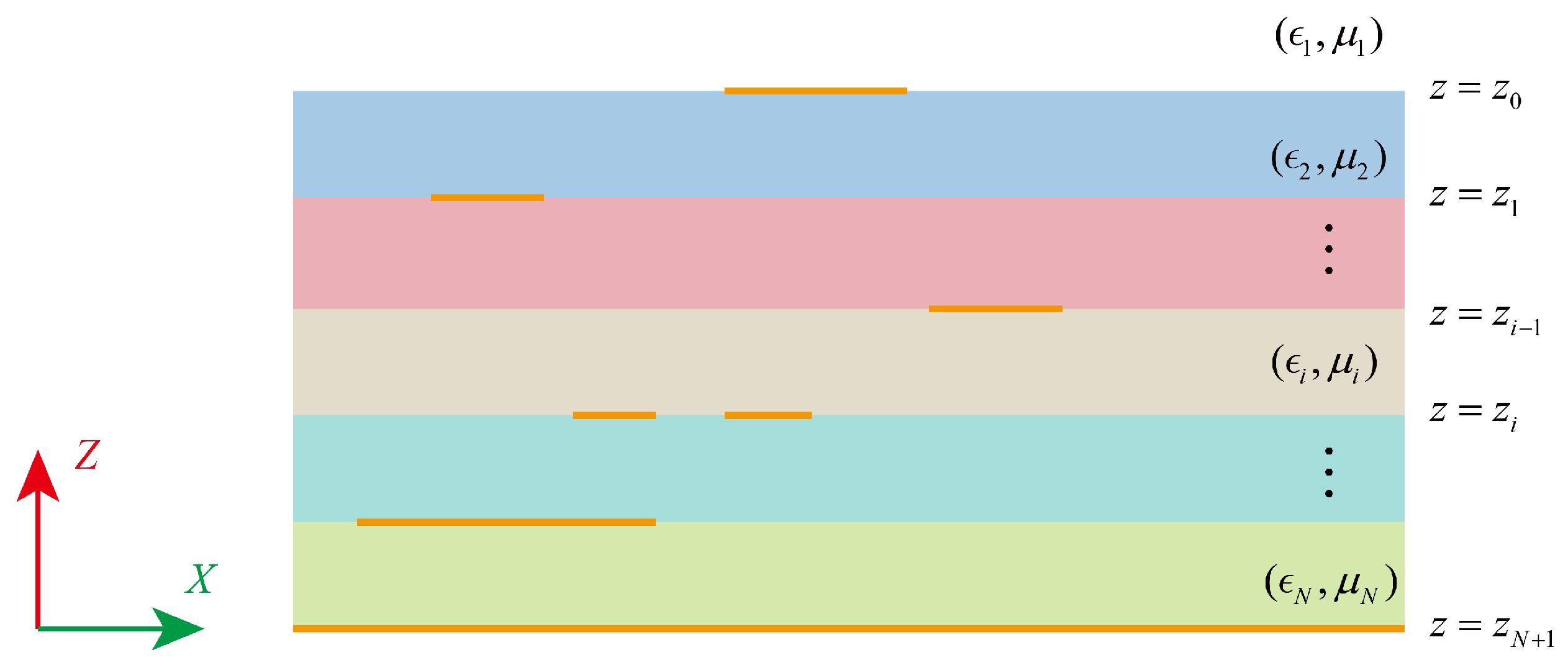
2. Theory and Formulations
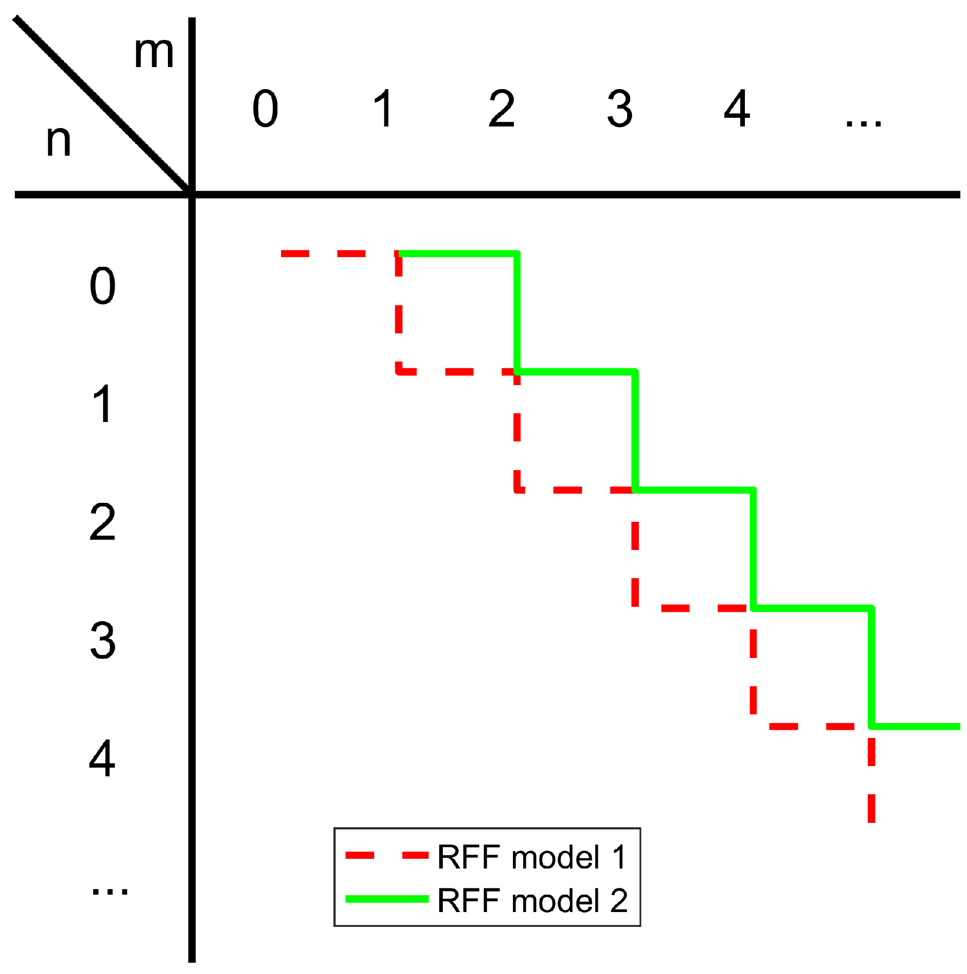
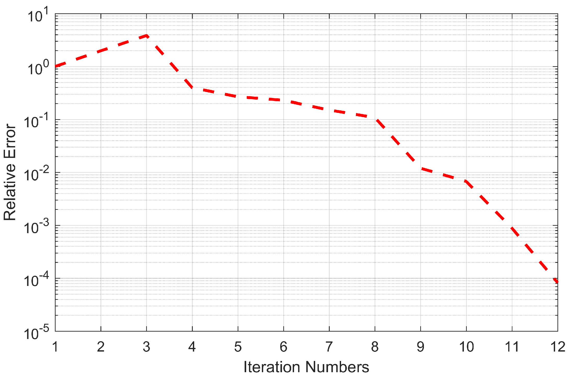
2.1. Proposed Adaptive RFFT
| Algorithm 1: Adaptive RFF for SIs |
 |
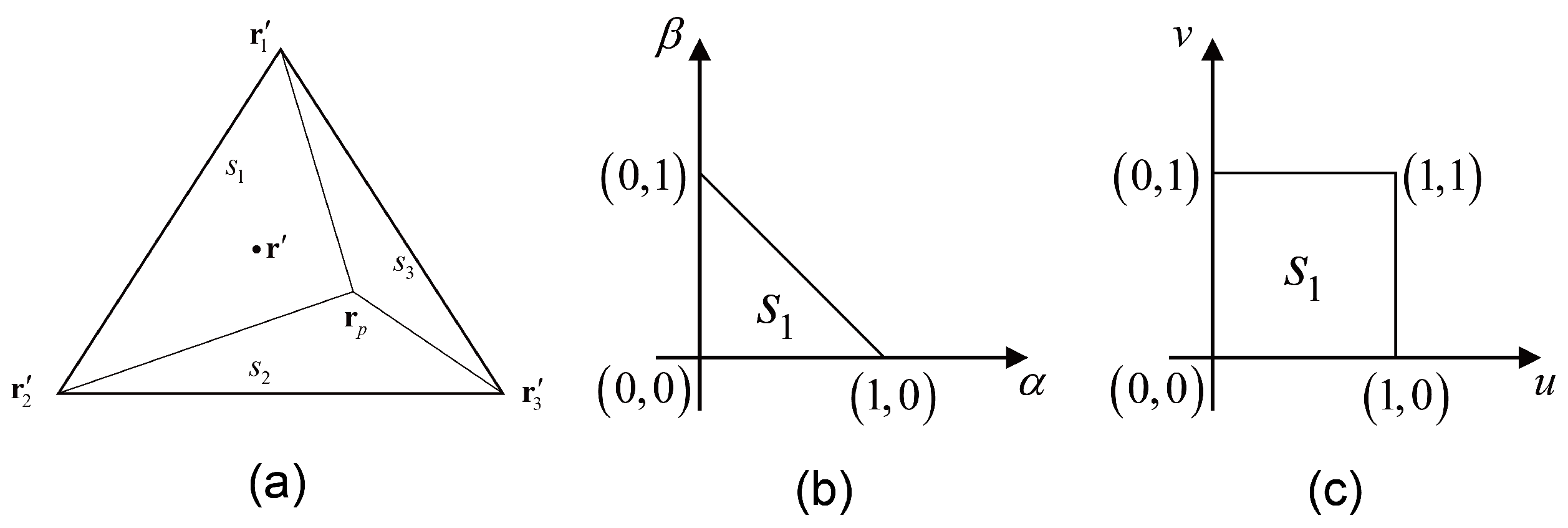
2.2. Singularity Treatment
- If lies on the direction vector , i.e., , we can define scalar , and the integral can be analytically evaluated. The detailed expressions given in Appendix B depend on the value of p.
- If is far from vector , the above integral has to be evaluated numerically using adaptive Gaussian integration.
- If is close to vector but not lies on it, to avoid the numerical integration for almost singular integrand as approx to zero, here we use the approximated conditionthen derive the approximated analytical expression for as shown in Appendix B.
3. Numerical Validation
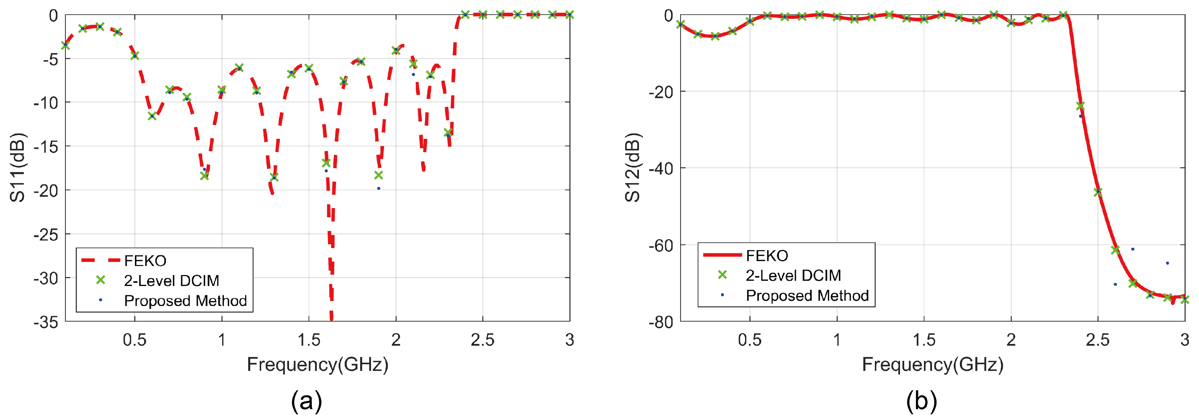
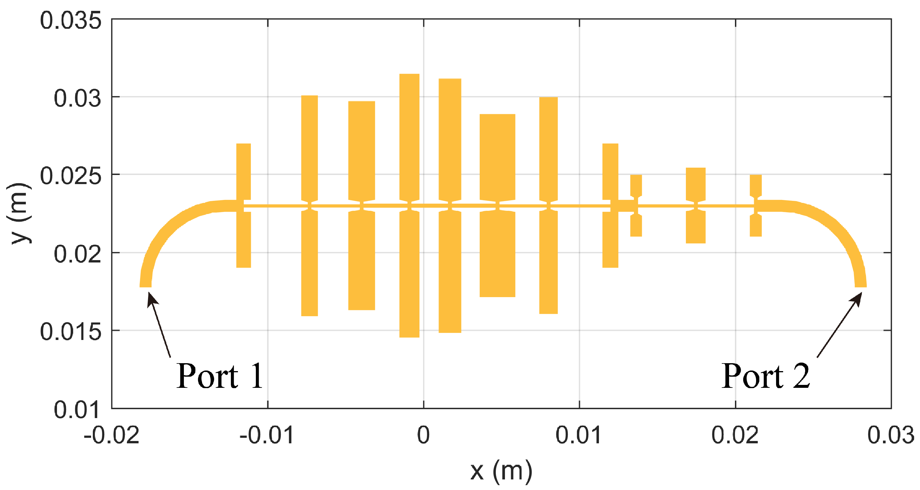
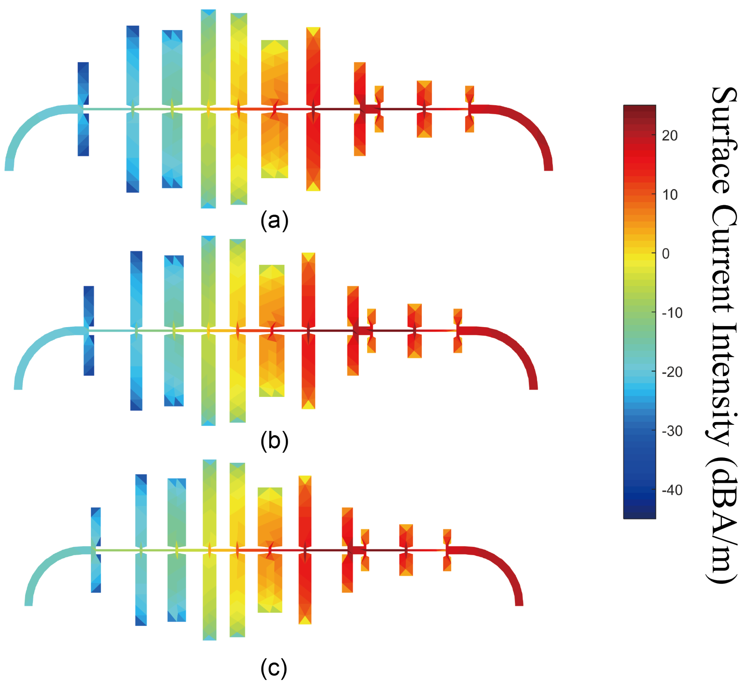
3.1. A Microstrip Low-Pass Filter
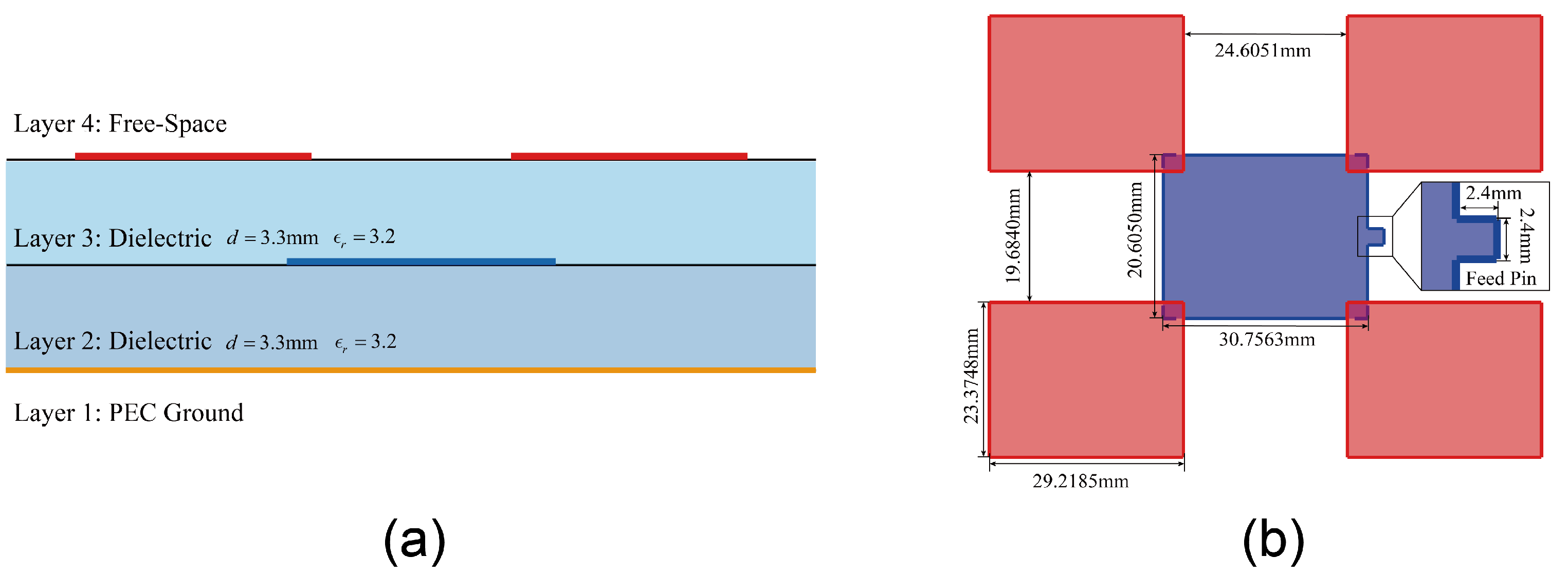
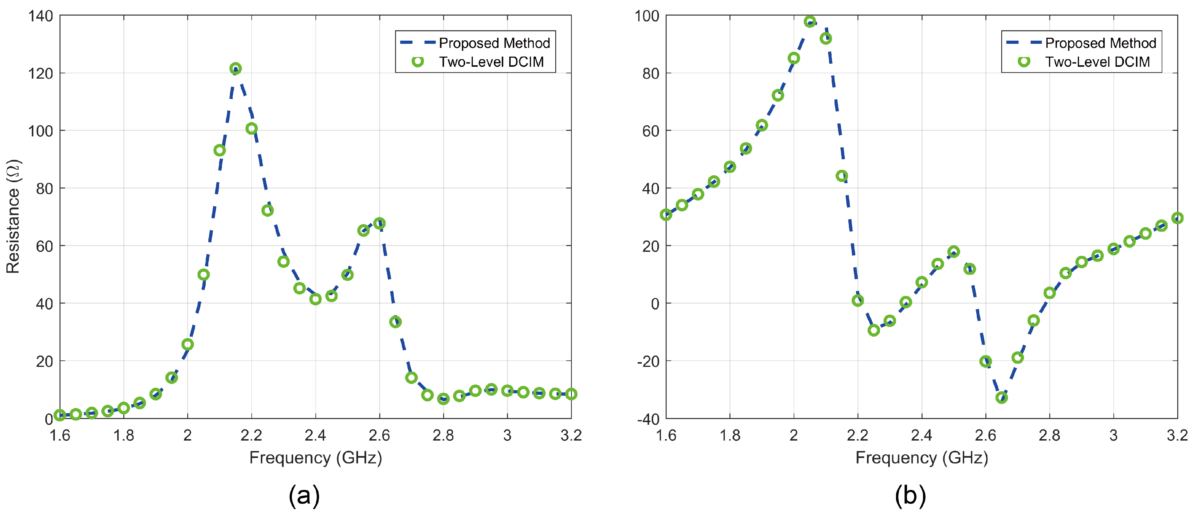
3.2. A Stacked Antenna
4. Conclusions
Author Contributions
Funding
Data Availability Statement
Acknowledgments
Conflicts of Interest
Appendix A
Appendix B
Appendix C
References
- Garg, R.; Bhartia, P.; Bahl, I.J.; Ittipiboon, A. Microstrip Antenna Design Handbook; Artech House: Norwood, MA, USA, 2001. [Google Scholar]
- Peixeiro, C. Microstrip patch antennas: An historical perspective of the development. In Proceedings of the 2011 SBMO/IEEE MTT-S International Microwave and Optoelectronics Conference (IMOC 2011), Natal, Brazil, 29 October–1 November 2011; pp. 684–688. [Google Scholar]
- Edwards, T.C.; Steer, M.B. Foundations for Microstrip Circuit Design; John Wiley & Sons: Hoboken, NJ, USA, 2016. [Google Scholar]
- MOSIG, J.R.; MICHALSKI, K.A. Sommerfeld integrals and their relation to the development of planar microwave devices. IEEE J. Microwaves 2021, 1, 470–480. [Google Scholar] [CrossRef]
- Mittra, R.; Ozgun, O.; Li, C.; Kuzuoglu, M. Efficient Computation of Green’s Functions for Multilayer Media in the Context of 5G Applications. In Proceedings of the 2021 15th European Conference on Antennas and Propagation (EuCAP), Dusseldorf, Germany, 22–26 March 2021; pp. 1–5. [Google Scholar]
- Winton, S.C.; Kosmas, P.; Rappaport, C.M. FDTD simulation of TE and TM plane waves at nonzero incidence in arbitrary layered media. IEEE Trans. Antennas Propag. 2005, 53, 1721–1728. [Google Scholar] [CrossRef]
- Zhang, K.; Goddard, L.L.; Jin, J.M. Efficient large-scale scattering analysis of objects in a stratified medium. Int. J. Numer. Model. Electron. Netw. Devices Fields 2020, 33, e2656. [Google Scholar] [CrossRef]
- Sercu, J.; Fache, N.; Libbrecht, F.; Lagasse, P. Mixed potential integral equation technique for hybrid microstrip-slotline multilayered circuits using a mixed rectangular-triangular mesh. IEEE Trans. Microw. Theory Tech. 1995, 43, 1162–1172. [Google Scholar] [CrossRef]
- Michalski, K.A.; Mosig, J.R. Multilayered media Green’s functions in integral equation formulations. IEEE Trans. Antennas Propag. 1997, 45, 508–519. [Google Scholar] [CrossRef]
- Tarricone, L.; Mongiardo, M.; Cervelli, F. A quasi-one-dimensional integration technique for the analysis of planar microstrip circuits via MPIE/MoM. IEEE Trans. Microw. Theory Tech. 2001, 49, 517–523. [Google Scholar] [CrossRef]
- De Donno, D.; Esposito, A.; Monti, G.; Tarricone, L. MPIE/MoM acceleration with a general-purpose graphics processing unit. IEEE Trans. Microw. Theory Tech. 2012, 60, 2693–2701. [Google Scholar] [CrossRef]
- Michalski, K.A. On the scalar potential of a point charge associated with a time-harmonic dipole in a layered medium. IEEE Trans. Antennas Propag. 1987, 35, 1299–1301. [Google Scholar] [CrossRef]
- Michalski, K.A.; Zheng, D. Electromagnetic scattering and radiation by surfaces of arbitrary shape in layered media. I. Theory. IEEE Trans. Antennas Propag. 1990, 38, 335–344. [Google Scholar] [CrossRef]
- Chen, Y.P.; Jiang, L.; Qian, Z.G.; Chew, W.C. An augmented electric field integral equation for layered medium Green’s function. IEEE Trans. Antennas Propag. 2010, 59, 960–968. [Google Scholar] [CrossRef]
- Ren, Y.; Zhao, S.W.; Chen, Y.; Hong, D.; Liu, Q.H. Simulation of Low-Frequency Scattering From Penetrable Objects in Layered Medium by Current and Charge Integral Equations. IEEE Trans. Geosci. Remote. Sens. 2018, 56, 6537–6546. [Google Scholar] [CrossRef]
- Ren, Y.; Zhao, X.; Lin, Z.; Chen, Y.; Meng, M.; Liu, Y.; Zhao, H. A Quasi-Mixed-Potential Layered Medium Green’s Function for Non-Galerkin Surface Integral Equation Formulations. IEEE Trans. Antennas Propag. 2022, 70, 2070–2081. [Google Scholar] [CrossRef]
- Michalski, K.A. Extrapolation methods for Sommerfeld integral tails. IEEE Trans. Antennas Propag. 1998, 46, 1405–1418. [Google Scholar] [CrossRef]
- Michalski, K.A.; Mosig, J.R. Efficient computation of Sommerfeld integral tails–methods and algorithms. J. Electromagn. Waves Appl. 2016, 30, 281–317. [Google Scholar] [CrossRef]
- Fang, D.; Yang, J.; Delisle, G. Discrete image theory for horizontal electric dipoles in a multilayered medium. In Proceedings of the IEE Proceedings H-Microwaves, Antennas and Propagation; IET: Stevenage, UK, 1988; Volume 135, pp. 297–303. [Google Scholar]
- Dural, G.; Aksun, M.I. Closed-form Green’s functions for general sources and stratified media. IEEE Trans. Microw. Theory Tech. 1995, 43, 1545–1552. [Google Scholar] [CrossRef] [Green Version]
- Okhmatovski, V.I.; Cangellaris, A.C. Evaluation of layered media Green’s functions via rational function fitting. IEEE Microw. Wirel. Components Lett. 2004, 14, 22–24. [Google Scholar] [CrossRef]
- Valerio, G.; Baccarelli, P.; Paulotto, S.; Frezza, F.; Galli, A. Regularization of mixed-potential layered-media Green’s functions for efficient interpolation procedures in planar periodic structures. IEEE Trans. Antennas Propag. 2009, 57, 122–134. [Google Scholar] [CrossRef]
- Wu, B.Y.; Sheng, X.Q. A complex image reduction technique using genetic algorithm for the MoM solution of half-space MPIE. IEEE Trans. Antennas Propag. 2015, 63, 3727–3731. [Google Scholar] [CrossRef]
- Alatan, L.; Aksun, M.; Mahadevan, K.; Birand, M.T. Analytical evaluation of the MoM matrix elements. IEEE Trans. Microw. Theory Tech. 1996, 44, 519–525. [Google Scholar] [CrossRef]
- Alparslan, A.; Aksun, M.I.; Michalski, K.A. Closed-form Green’s functions in planar layered media for all ranges and materials. IEEE Trans. Microw. Theory Tech. 2010, 58, 602–613. [Google Scholar] [CrossRef]
- Stoer, R.B.J. Introduction to Numerical Analysis, 3rd ed.; Texts in Applied Mathematics 12; Springer: New York, NY, USA, 2002. [Google Scholar]
- Press, W.H.; Teukolsky, S.A.; Vetterling, W.T.; Flannery, B.P. Numerical Recipes: The Art of Scientific Computing, 3rd ed.; Cambridge University Press: Cambridge, UK, 2007. [Google Scholar]
- Khayat, M.A.; Wilton, D.R. Numerical evaluation of singular and near-singular potential integrals. IEEE Trans. Antennas Propag. 2005, 53, 3180–3190. [Google Scholar] [CrossRef]


| Spatial Region | Proposed Method | DCIM | |||
|---|---|---|---|---|---|
| Execution | 0.53 | 0.53 | 0.18 | 0.16 | |
| CPU time (ms) | 0.62 | 0.66 | |||
| Number of terms | 9 | 8 | 13 | 10 | |
| 11 | 11 | ||||
| CPU time (ms) | 4.34 | 4.40 | 37.6 | 29.0 | |
| for SI evaluation | 4.87 | 5.32 | 37.4 | 28.4 | |
| Relative error 1 | 9.9 × 10⁻⁴ | 1.4 × 10⁻⁴ | 1.0 × 10⁻³ | 2.6 × 10⁻⁴ | |
| 2.8 × 10⁻⁵ | 2.5 × 10⁻⁵ | 6.7 × 10⁻⁵ | 6.5 × 10⁻⁵ | ||
| Spatial Region | Proposed Method | DCIM | |||
|---|---|---|---|---|---|
| Execution | 0.55 | 0.56 | 0.15 | 0.16 | |
| CPU time (ms) | 0.35 | 0.36 | |||
| Number of terms | 8 | 10 | 45 | 45 | |
| 5 | 5 | ||||
| CPU time (ms) | 4.18 | 4.47 | 95.4 | 101.0 | |
| for SI evaluation | 4.05 | 4.01 | 99.2 | 102.9 | |
| Relative error 1 | 2.6 × 10⁻³ | 3.8 × 10⁻³ | 2.7 × 10⁻³ | 3.8 × 10⁻³ | |
| 4.9 × 10⁻⁴ | 6.9 × 10⁻⁶ | 7.2 × 10⁻³ | 8.9 × 10⁻⁵ | ||
| Proposed Method | DCIM | |||
|---|---|---|---|---|
| Fill Matrix | Total Time | Fill Matrix | Total Time | |
| Low-Pass Filter | 1445 | 1599 | 9659 | 9818 |
| Stacked Antenna | 1104 | 1227 | 7056 | 7161 |
Publisher’s Note: MDPI stays neutral with regard to jurisdictional claims in published maps and institutional affiliations. |
© 2022 by the authors. Licensee MDPI, Basel, Switzerland. This article is an open access article distributed under the terms and conditions of the Creative Commons Attribution (CC BY) license (https://creativecommons.org/licenses/by/4.0/).
Share and Cite
Zhao, Z.-H.; Wu, B.-Y.; Li, Z.-L.; Yang, M.-L.; Sheng, X.-Q. An Adaptive Rational Fitting Technique of Sommerfeld Integrals for the Efficient MoM Analysis of Planar Structures. Electronics 2022, 11, 3940. https://doi.org/10.3390/electronics11233940
Zhao Z-H, Wu B-Y, Li Z-L, Yang M-L, Sheng X-Q. An Adaptive Rational Fitting Technique of Sommerfeld Integrals for the Efficient MoM Analysis of Planar Structures. Electronics. 2022; 11(23):3940. https://doi.org/10.3390/electronics11233940
Chicago/Turabian StyleZhao, Zi-Hao, Bi-Yi Wu, Ze-Lin Li, Ming-Lin Yang, and Xin-Qing Sheng. 2022. "An Adaptive Rational Fitting Technique of Sommerfeld Integrals for the Efficient MoM Analysis of Planar Structures" Electronics 11, no. 23: 3940. https://doi.org/10.3390/electronics11233940