Article

Location Based Indoor and Outdoor Lightweight Activity Recognition System

1
DeustoTech Institute of Technology, University of Deusto, Av. Universidades 24, 48007 Bilbao, Spain
2
Department of Engineering for Innovation, University of Salento, Via Monteroni snc, 73100 Lecce, Italy
*
Author to whom correspondence should be addressed.
These authors contributed equally to this work.
Electronics 2022, 11(3), 360; https://doi.org/10.3390/electronics11030360
Submission received: 31 December 2021 / Revised: 19 January 2022 / Accepted: 21 January 2022 / Published: 25 January 2022

Abstract

:
In intelligent environments one of the most relevant information that can be gathered about users is their location. Their position can be easily captured without the need for a large infrastructure through devices such as smartphones or smartwatches that we easily carry around in our daily life, providing new opportunities and services in the field of pervasive computing and sensing. Location data can be very useful to infer additional information in some cases such as elderly or sick care, where inferring additional information such as the activities or types of activities they perform can provide daily indicators about their behavior and habits. To do so, we present a system able to infer user activities in indoor and outdoor environments using Global Positioning System (GPS) data together with open data sources such as OpenStreetMaps (OSM) to analyse the user’s daily activities, requiring a minimal infrastructure.

1. Introduction

In smart environments one of the most relevant information that can be gathered about users is their position. Continuous monitoring of user’s location is crucial when it comes to the development of accurate activity recognition and behavior modeling systems. Nowadays, it is very common to see applications for different purposes using indoor and outdoor positioning systems, including data-driven and knowledge-based methods for monitoring the behavior of elderly people. Therefore, user behavior modeling is one of the most important tasks in intelligent environments [1]. To be aware of what the user is doing and how it is performing the different tasks is essential to be able to properly adapt to their need. Behavior modeling has been used to address problems in different tasks: to adapt and control the energy consumption of the intelligent environments [2], create context-aware smart cities [3,4] or early risk detection related to different pathologies [5,6].
One of the main issues when applying behavior modeling techniques is the required underlaying sensor infrastructure to infer the activities they are performing. Most of the activity recognition and behavior modeling approaches rely on dense sensing environments that rely either in physical sensors (passive infrared sensors, contact sensors, smart plugs…) or video to recognize the activities that are being performed by the users, increasing the initial requirements and overall costs of such systems, becoming even more demanding if the final objective is to also recognize the behavior in outdoors, like in a smart city scenario. Accordingly, there are situations where an environment has been adapted to users with special needs or pathologies where having a dense sensor infrastructure is justified.
To address those situations, we propose an extension of our previous work [7] on location-based activity recognition systems in two environments: indoor and outdoor. When it comes to the outdoor positioning system, we exploit the semantic location data exposed in services like OSM to identify the activities that the user is performing. Even though the developed behavior model is simpler and less granular than those that need a more complex infrastructure, in this case the hardware requirements are minimal, only a mobile device. Furthermore, one additional benefit of the system we propose is that reduces the burden for the users, getting advantage of the mobile phone, a device that most users are already have with them all the time, not requiring of additional gadgets. To do so, the proposed system consists of two modules: the Point of Interests (POI) identification and semantic location extraction modules. The first one gets as input the location history of a user (GPS coordinates gathered every minute) and applies some data cleaning and clustering processes that are described in depth in the corresponding section, in order to identify those POIs that the user has visited. Then, the semantic location extraction module analyses the previously identified POIs so that we can infer the activities that the user has carried out. To do so, we have developed a building partitioning method in order to improve the performance of the reverse geocoding tool provided by Nominatim (https://github.com/osm-search/Nominatim (accessed on 19 January 2022)), the public Application Programming Interface (API) of OSM.
Secondly, the indoor positioning system is mainly based on Bluetooth Low Energy (BLE) technology that can provide information about the user’s location in different places (home, stores, malls, etc.). The system requires minimal infrastructure at low cost. Such a system can extend the proposed method to provide a more comprehensive solution in mixed environments where the indoor positioning in places like a home is also needed.
The rest of the paper is organized as follows. Section 2 summarizes the related work on indoor and outdoor activity recognition. Section 3 describes the developed outdoor activity recognition system and Section 4 the indoor activity recognition system. In Section 5 we discuss about the developed approaches. Finally, Section 6 presents our conclusions and lines of future work.

2. Related Work

Due to the high spread of services offered by innovative technologies, such as the one introduced by the Internet of Things (IoT) domain, during the last decade the research community has started to investigate and propose techniques, tools and solutions to predict users’ behavior and recognize their current and future activities. Nowadays, the city and its facilities have been enhanced by services that allow users to live more fruitful days and enjoy their lives. The possibility of knowing the exact current position of the bus to reach the city center or avoiding the traffic while we are driving a car are only some examples of all the advantages for citizens brought thanks the new services introduced in the smart cities. Nonetheless, most of these duties base their functionalities on the monitoring of both the environment and the users themselves and sometimes fail simply because they cannot interpret the next actions of the user (e.g., a system could suggest to avoid a road that seems to be full but it is exactly the destination of all the cars that are occupying and so it could cause a delay that would have been avoided by predicting the destination of the occupants). These reasons motivate the research conducted to predict users’ behavior and recognize their current and future activities [8,9,10,11,12]. As demonstrated by the various works presented in the literature, thanks to such predictions it is possible to enhance a multitude of existing services, such as improving logistics in different domains [13,14,15], reimagine and dynamically repurpose built environment or customize services [16,17], prevent and manage dangerous situations [18,19,20,21,22], but also their provision. Related to this last aspect, the works proposed in [23,24] demonstrate how the prediction of the user behavior and activities could help in predicting and consequently mitigate the resource demand in a particular moment to distribute the network bandwidth and the processor load dedicated to that service.
Different techniques have already been proposed in the literature aimed to recognize the user behavior [25,26,27,28] but only a few of them exploit innovative techniques based on POIs or semantic location as done in the proposed paper, and, to the best of our knowledge, none of them combine both techniques as part of our previous works that inspired the present one [7]. Therefore, the present paragraph will be divided into two main parts: the first one is dedicated to the techniques that exploit POI while the second one is focused on the one handling semantic location.
In [29], the work proposed by authors is based on the Location-Based Social Network (LBSN) concept. A LBSN is a new social structure made up of individuals connected by the interdependency derived from their physical locations as well as their location-tagged media content, such as photos, video, and texts, that is created by adding a location to an existing social network so that people in the social structure can share location embedded information. The physical location in this context consists of an individual’s instant location at a given timestamp and the location history that an individual has accumulated over a given period. Furthermore, interdependence encompasses not only the fact that two people co-occur in the same physical location or share similar location histories, but also knowledge, such as common interests, behavior, and activities, inferred from an individual’s location (history) and location-tagged data. In particular, the authors propose an algorithm based on tree-based hierarchical graph (TBHG) and Hyperlink-Induced Topic Search (HITS) algorithm considering GPS trajectories model to infer users’ travel experiences and interest of a location within a region. By analyzing the POI of the selected scene perception task, authors are capable to find that those users have similar POI and rank them by the location and experience using the proposed algorithm.
The concept presented in [30] is to use existing Location-Based Services (LBS) infrastructure to track the user and achieve other system navigation goals. The information source is the freely available and up-to-date internet infrastructure. Initially, conventional methods are used to determine the user’s location. The semantic labels are used and associated with the underlying location in order to relate the location with the web content. The semantic labels are obtained through reverse geocoding, which returns the names of local attractions, streets, cities, states, and countries, etc. The labels are then used to search for the associated detailed content in the web. The region data is kept in two places: a locally populated database and a web database. In the LBSN, community detection techniques are useful for social media algorithms to discover people with common interests and keep them tightly connected. Community detection can be used in machine learning to detect groups with similar properties and extract groups for various reasons.
In [31] community detection is applied to explore the friendship circles among the users and within each friendship circle recommend POI for each user. In [32] a model of human mobility that reliably predicts the locations and dynamics of future human movement using cell phone location data, as well as data from two online location-based social networks is presented.
With regard to the use of the meanings of the locations, in [33] an effective POI recommendation method for LBSNs based on collaborative filtering is described. The proposed method focuses on inferring user’s check-in behaviors from user’s location history to make a high-quality recommendation of POIs to a user based on the current location and opinions of similar users. The model is validated using two real-world datasets collected from Foursquare.
To enable analysis of movement behavior, in [34,35] authors present an approach to enrich trajectory data with semantic POI information and show how additional insights can be gained. In particular, a stepwise approach to generate insights from recorded vehicle movements is presented. Authors first processed a massive movement dataset and extracted frequent and dense destination areas. Then, they enriched the data with context information using Foursquare. The proposed model is evaluated with two case studies on a large electric scooter data set and tested on data with known ground truth.
In [36] an automatic Semantic Location History (SLH) construction system is presented, named iManer. It consists of an improved Kalman filter-based approach to obtain accurate location and heading estimation from inertial sensor readings of smartphones. The collected users’ location and heading histories are further mined to estimate Areas of Interaction (AoI).
In order to integrate heterogeneous location aware systems into ubiquitous computing environment, in [37] authors present a novel semantic location-aware model based on ontology. The proposed model can share, reason, and manage context information and services in a spatial containment relationship and adjusting the usage policies of services dynamically. In [38] addresses location issues in ubiquitous mobile computing and presents a semantic location model that incorporates query and context semantics in a user-centered model to support context-aware cooperative mobile events. To recognize and use semantics, an event-reasoning mechanism based on semantic matching is established. A natural language query is defined, and a prototype is discussed as a scenario for evaluating the location model, resolving the perplexing problem of converting from linguistics to semantics, and then to pragmatics.
The approach proposed in [39] extends that used in semantic GIServices to LBSs, while keeping context in mind. Contextual information is linked to information, action, and user spaces. It is composed of five elements: user, location, time, event, and object. A framework is presented based on the context model to accommodate semantics in both LBS and GIServices. In LBS, the context-aware framework facilitates information discovery, access, and composition.
In terms of indoor localization systems based on wireless access points, these approaches measure the intensity of the received signal [40] and the fingerprinting method [41,42] used to infer the user’s location. Because of its low cost, small form factor, and ability to communicate without a battery, Radio Frequency Identification (RFID) has been considered an IoT enabler technology. This technology enables people and smart objects to connect digitally, be identified, and tracked [43]. Furthermore, it is primarily employed for supply chain traceability [44], including some critical supply chains such as [45,46,47]. However, this is not their only use, nowadays RFID is also used for localization in several contexts. For example, in the medical field, this IoT enabler can be used to collect information on patients who require home care, allowing them to be located within their homes and analyzing their behavior [48].
Furthermore, in recent years, Bluetooth has become one of the most popular indoor location technologies. Bluetooth positioning technologies among others [49,50], depending on its configuration and enhancements, can provide accuracy down to meters or even centimeters. Consequently, it adapts better to tasks where pinpoint accuracy is not necessary. Moreover, aside from its low cost and ease of use, BLE-based positioning technology can produce reliable results. For instance, BLE has been used in museums and galleries to guide the visitors and provide information about the artworks [51,52]. This method of indoor positioning is based on Bluetooth Low Energy beacons that are attached to objects, walls, and other surfaces and emit radio signals at predetermined intervals. These battery-powered devices communicate with other Bluetooth-enabled devices, such as smartphones. An application on the user’s device (e.g., smartphone, tablet, smartwatch) detects Bluetooth signals and uses the Received Signal Strength Indicator (RSSI) to calculate the distance to the BLE beacon.
Furthermore, newer Bluetooth versions have improved location services. The new Bluetooth 5.1 direction-finding feature, which uses the Angle of Arrival (AoA) and Angle of Departure (AoD), improves accuracy down to the centimeter level [53], allowing the development of a diverse range of reliable and accurate indoor positioning solutions and applications. In Table 1, an overview of methods and technologies used in the related studies is presented.

3. Outdoor Activity Recognition System

To address this task, we have developed a location-based activity modeling mechanism that exploits the semantic location data exposed in OSM to identify the activities that the user is performing. The designed outdoor activity recognition system is divided into two steps or modules: the Point of Interests identification module and the semantic location extraction module.

3.1. POI Identification Mechanism

In this section, we are going to introduce the developed POI identification system. This module gets as input the daily points of the user that the used mobile application has been able to gather. The application collects location information every 1 min, therefore, in a single day we would have to process 1440 sequential GPS coordinates (60 min × 24 h). Once this module receives the daily location data, it pre-processes the raw data to handle any GPS inaccuracies and time intervals without any data (the smartphone was switched off or without internet connection for various days). Then, we take advantage of the Density-Based Spatial Clustering of Applications with Noise (DBSCAN) [54] clustering algorithm, adapting it to this specific task. Finally, we start the creation of a location-based daily activity timeline for the user. This module has gone through two iterations that we are going to explain in the following sections in order to clarify the reasoning behind this decision, giving some insight about how and why we have implemented the proposed changes in the second iteration.

3.1.1. First Iteration

First, the GPS data is cleaned to fix some of the issues found when it comes to smartphone’s GPS accuracy. The first issue is the GPS drifts, when suddenly the smartphone reports for an unspecified period (usually a few minutes) a location that is far away from the real one and then returns to the real location. During the development of the data cleaning process we found that there can be different types of GPS drifts which sometimes can be mistaken for actual coordinates. To fix this, for each consecutive three points we check if the following three conditions are true. These conditions were defined after analyzing the pattern of several GPS drifts found in the data gathered from different volunteers. Therefore, if the three conditions are fulfilled, a GPS drift is found (see in Figure 1 the three points that form the marked triangle):
  • The angle formed by connecting the three points is less than 40 degrees.
  • The ratio between the two sides of the angle (longest side/shortest side) is less than 2.
  • The angles formed by the first point and its previous point, or the angle formed by the third point and its next point, are greater than 145 degrees and less than 215 degrees.
The second issue detected is that there are some cases where the phone stops updating the coordinates and therefore, the coordinates are the same for a few minutes. When this happens, all the points will be unified in a single one with a larger duration.
After the raw data has been properly cleaned, DBSCAN clustering algorithm has been used to identify the most relevant clusters and analyze if those clusters can be selected as a POI. The parameters used in this case are eps (the maximum distance between two samples to be considered as neighbors) of 25 m, minimum samples (the minimum number of points each cluster should have) to one, ball tree as algorithm and haversine as metric. DBSCAN returns a label per each of the points fed into it. Therefore, those points belonging to the same cluster would have the same label, whereas those points that do not belong to any cluster would have a unique label. Until this point, only the geographical data have been taken into account. However, there is also temporal data that should be used too. To do so, the GPS data is analysed in temporal order checking if the next point’s label is the same as the previous one, unifying all consecutive points with the same cluster label until a point with a different label is found. Therefore, those consecutive points, which belong to the same cluster, are grouped together being the duration of the cluster the addition of all points’ durations. Finally, a cluster is considered a POI if the user has been there more than 5 min.
Testing and validation. Using the algorithm described above, a first prototype is implemented and tested with data from real mobile devices from some volunteers. These tests were created after manually annotating specific days of the gathered data that we considered could help in the evaluation of the proposed system due to their characteristics: high mobility days or large number of GPS inaccuracies that were found after a manual analysis of the data. In general terms, the obtained results were acceptable, but there were occasions in which the mobile devices, especially when they were indoors, captured erroneous GPS points that showed erratic results and the implemented data cleaning algorithm was not able to correct them. Including the errors identified before, the GPS errors detected are summarized into three types:
1.
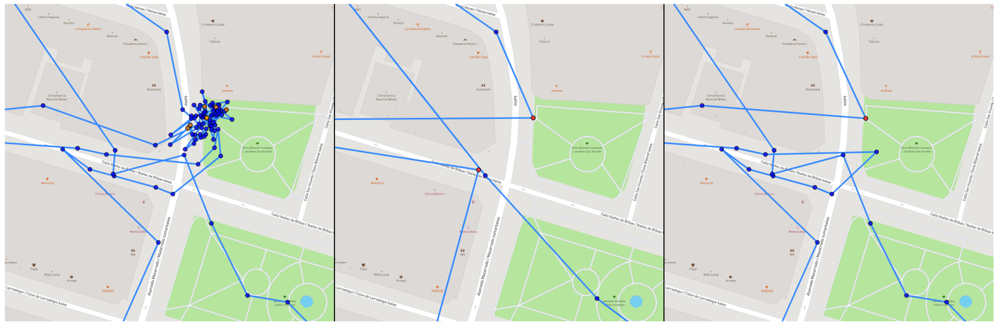
Static jumps: already identified during the data cleaning phase of the first iteration. They are points that have exactly the same coordinates. It is not common for the points to have the same coordinates; therefore, they may indicate that there are errors in the GPS data (See Figure 2).
2.
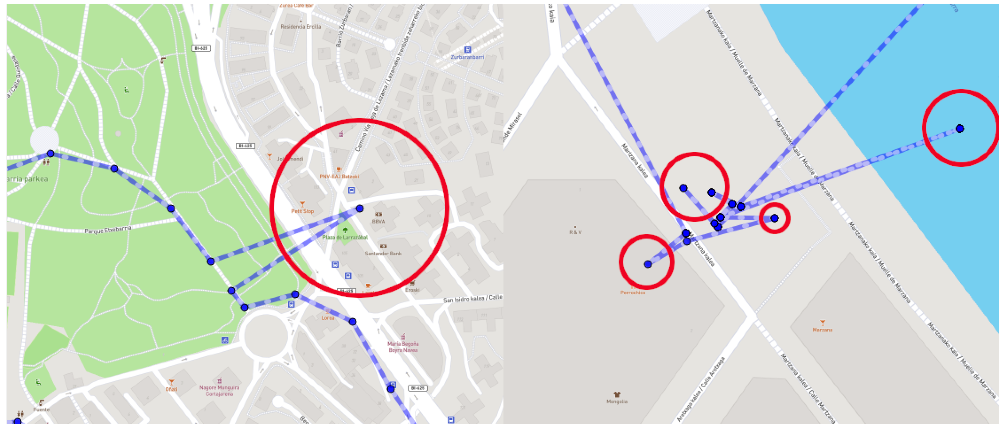
GPS drifts: also addressed during the first iteration. However, the data cleaning algorithm was mainly oriented to motion-related GPS drifts. After analysis of results, another more problematic type of GPS drift associated with static points was detected (See Figure 3).
3.
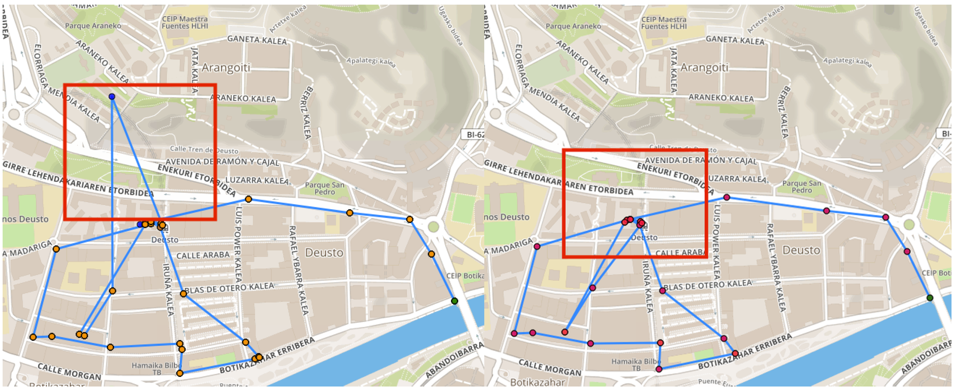
Multi-clustering: even though it is directly related to the two previous errors, multi-clustering is so relevant that it has to be addressed in a different way. Sometimes, due to GPS errors, although the user remains in the same place, spatial jumps (in the form of drifts or static-jumps) occur, resulting in false clusters, when in fact all the points belong to the same unique cluster (see Figure 4 where all the points belong to a single cluster).
The data cleaning algorithm developed for the first iteration was suitable for GPS drifts that take place when there is motion, so it can detect and clean points that appear anomalously in the current user’s trajectory. However, when the GPS drifts take place statically (i.e., when the user is at home), this algorithm is not reliable. These kinds of drifts usually have a zigzag shape (going and returning several times) so the algorithm is unable to determine which of the points is the correct one and which one is the drift. A clear example of this problem can be seen in Figure 5.
Also, the detected multi-clustering problem invalidated the clustering system developed during the first iteration, since all those false clusters generated by GPS errors were considered real clusters, reducing the reliability and accuracy of the algorithm.

3.1.2. Second Iteration

Due to the issues detected in the testing phase, we decided to re-evaluate the process and implement a new clustering algorithm using the lessons learned in the first iteration but trying to correct the problems detected. First, it was decided not to use the initial cleaning step implemented in the first iteration because we detected that it was not able to deal with all the different types of GPS drifts that we have identified during the development of the system. Consequently, using the output route of this process could have led to an error that would have been spread throughout the following steps of the process.
The new procedure could be divided into three phases: pre-processing, where the necessary data for clustering is obtained, the multi-clustering algorithm itself, and a final post-processing phase where the route is cleaned.
Pre-processing. First, we run the DBSCAN algorithm to identify high quality clusters. In this step, the parameters used in the first iteration are modified. We used a more restrictive eps of just 9 m (instead of 25 m), and a minimum of five samples are required for a cluster to be considered as such. In this way, the detected clusters receive a numerical label and the points that do not belong to any cluster receive the label ‘−1’.
Next, the quality of the clusters obtained is evaluated. As discussed during the explanation of the POI detection system of the first iteration, DBSCAN is particularly suitable for detecting clusters from a geographical point of view, but in our case, as a user may walk several times through a geographical area at different times of the day, DBSCAN may erroneously identify those points as belonging to the same cluster. Therefore, we analyze each detected cluster and determine if it can be considered as ‘good’ (indeed, it is going to be a cluster), or ‘bad’ (either because it is not really a cluster, or because it is composed of several temporal clusters sharing geographic space).
The following characteristics are obtained for this evaluation:
  • The standard deviation of the distances from the cluster points to the cluster centroid. In general, a good cluster should not have values that are too high (something that is already taken care of by DBSCAN itself), but not too small either as it would imply a “static jump”.
  • The variability representing the average number of different coordinates with respect to the total number of points in the cluster. In a good cluster it is not normal that coordinates are repeated, therefore, it is normal to have values close to 1. If they are closer to 0, it implies a “static jump”.
  • Number of inputs and outputs. The number of inputs and outputs occurring in that cluster is checked. A good cluster should have 2, if it is in the middle of the route, or 1 if it is the start or the end of the route (home, for example). A larger number may imply that the same cluster is crossed by the user several times throughout the day, although it could also be the result of a GPS drift that goes outside the cluster boundaries.
  • Time jumps inside the cluster. The time difference between consecutive points in the cluster is calculated and those exceeding 125 s are considered as “time jumps” (GPS samples are usually obtained every 60 s, so we give a margin of slightly more than two samples).
With the available data, we manually evaluated our approach and based on the results obtained, we established the different thresholds that determine whether a cluster is ‘good’ or ‘bad’. These thresholds are intended to reduce the number of false positives so, when a cluster is considered ‘good’ we can have a high certainty that it is a real cluster.
  • First, those clusters that have two or less inputs and outputs are checked. When these clusters have a variability of less than 0.5 and the standard deviation of the distances is greater than 1.8, these clusters are considered as ‘good’. On the contrary, they are considered ‘bad’ when the standard deviation of the distances is less than 0.1 (regardless of the variability). For all other cases, the cluster is considered as ‘good’.
  • For those clusters that have more than two inputs and outputs, only the clusters that have no time jumps are considered ‘good’.
  • The clusters are considered as ‘bad’ for all other cases.
Once the stratification of the clusters has been performed, the labels assigned by DBSCAN are updated. Consecutive numerical labels (starting from the last detected cluster) are assigned to all points that have not been assigned to a cluster by DBSCAN. If several points have the same coordinates, they are considered part of the same cluster (this cluster is a ‘static jump’). A single GPS point that is not part of another cluster because it is a transition within the route will form a single point cluster. Then, the clusters are analyzed to verify if they are ‘static jumps’ (all points of the cluster have the same coordinates). Finally, a map of relationships between the different clusters is generated based on the inputs/outputs between the clusters. This information is especially relevant to try to detect the multi-clustering error described above.
Clustering. The points of the route are iteratively processed and we check if they are the starting point of a cluster based on the following algorithm (see Figure 6). In this algorithm, it is considered that a multi-cluster can have a maximum of 5 levels.
  • Level 1: The cluster analysis starts from level 1, so the label of the first point to check is considered the initial label of this level. Then, we get the next point and check if it belongs to the first level (it has a label that belongs to level 1). If not, it would go to level 2 (the label of this new point will be the initial label of level 2).
  • Level 2: The next point of the route is taken and its label is checked. If it is a label belonging to level 1, it is returned to level 1. As we consider that all the points until now are part of the same cluster, we add the labels of level 2 as valid levels for level 1. If the label is not part of level 1, we check if it belongs to the labels of level 2, in that case, we consider that the point still belongs to level 2. Otherwise, we check if the label is part of ‘good’ labeled cluster, since a good cluster cannot belong to a multi-cluster, the process is considered completed and the actual cluster is considered with only those points belonging to level 1. If the cluster is not labeled as ‘good’, it would go to level 3 (the label of the new point being the initial label of level 3).
  • Level 3: Again, we get the next point of the route and its label is checked. If it is a label belonging to level 1, it is returned to this level and the labels of levels 2 and 3 are added to level 1. On the contrary, if it is a label of level 2, it is returned to this level and the labels of level 3 are added to level 2. Otherwise, a preliminary check is made before moving to level 4. The centroids of the three levels are calculated and it is checked if any of them form an angle less than 45º, or level 3 has been labeled as a bad cluster, or it is a static point, in which case it is moved to level 4 (the label of the new point being the initial label of level 4). If the condition is not fulfilled, the process is finished and only the points belonging to level 1 would be part of the actual cluster.
  • Level 4: As in the other levels, the label of the next point on the route is checked. If it is a level 1 label, it is returned to this level and the labels of levels 2, 3, and 4 are added to level 1. If it is a level 2 label, it is returned to this level and the labels of levels 3 and 4 are added to it. Otherwise, and as long as the point label is not part of a cluster labeled as ’good’ (in which case the process ends directly), a previous check is made again before passing to level 5, if the current point label belongs to a cluster related to any of the clusters (labels) belonging to level 4, or if the current point is static, it is passed to level 5 (as always, using the label of this point as the initial label of level 5). If the condition is not fulfilled, the process ends, the rest of the levels do not belong to the cluster, and only the points belonging to level 1 are part of the real cluster.
  • Level 5: As in the previous case, the different levels are checked and the corresponding level is passed by updating the labels. If the tag belongs to level 5, it remains at the same level. Otherwise, the analysis is finished and only the level 1 points are part of the cluster.
The points obtained from the previous method can belong to more than one level, which implies clusters with different geographical coordinates but which are considered to belong to the same cluster. To determine the real centroid of this cluster, two DBSCAN calculations are performed on the points obtained, one with an eps of 5 m and the other one with 25 m, both with a minimum sample size of 1. In both cases, it is calculated which cluster agglutinates the highest number of points (ignoring static points), and the centroid is calculated from the points of this cluster. The ratio of the number of points represented by the centroid of eps05 and eps25 is checked. If the ratio is less than 0.5, the eps25 centroid is used (eps05 is too small and has lost precision), otherwise, esp05 is used. Once this process is finished, the route has been clustered. Now it is time to clean the static points and the GPS motion-drifts from the route (following the same algorithm that was used to clean the path in the first iteration).
Post-processing. After that, the small deviations from the user’s home are cleaned up. First, the home of the user is inferred clustering with DBSCAN the GPS coordinates between 1 AM and 6 AM and selecting as home the largest cluster. The points (or clusters) of the route are iteratively processed and, if the distance is less than a given threshold (30 m) and it is not a good cluster, the user is considered to be at home and the coordinates of the point (or cluster) are replaced by those of his home. This way, any time the user is at home, the points have homogeneous coordinates.
Then, a final pass of the clustering algorithm of the initial interaction is made as a final cleaning of the route, aggregating the different static points generated after analyzing the small deviation from the user’s home. Finally, we consider that a point of interest has been found if the user has stayed in the same place for a minimum of five minutes.
Testing and validation. Once the new algorithm developed in the second iteration has been completed, it is evaluated to measure its accuracy and efficiency. For this purpose, the samples with real mobiles obtained during the testing and evaluation phase of the first iteration are used. As expected, the previous results are improved without detecting any decrease in the efficiency of the previously corrected results. Next, we will see some examples comparing what is obtained directly from the mobiles, the result of the cleaning and clustering algorithm of the first iteration, and the result of the second iteration.
In Figure 7 we can see the same example (left) of static-related GPS drifts that was shown when we presented the different kinds of static drifts that we have detected. As it can be seen, there are several drifts (that are also static-jumps, indicated by the yellow dots). Both algorithms can correctly clusterize this kind of drift into one place (that will be a point of interest as the user has been there for more than five minutes).
In the example of Figure 8, we can see a big cluster of points (the big cloud of points on the left). Both algorithms can clusterize it correctly thanks to the underlying DBSCAN algorithm that both interactions use. However, the first-iteration erroneously clusterizes some other points that are not a real cluster but a change of trajectory of the user. Reducing the eps of the initial DBSCAN from 25 m to 9 m allows the second iteration to avoid making this mistake.
In Figure 9, we also see an example previously shown. In this case, we see (left) an example of zig-zag shaped static GPS drift that the data cleaning algorithm of the first iteration (center) is unable to remove. These kinds of drifts are really cumbersome and they need to be processed differently from other drifts. The multi-clustering algorithm developed in the second-iteration (right) can cope with these drifts correctly.
In the route that can be seen in Figure 10, we have a clear example of multi-clustering. At first, it seems it is a normal route, but after a thorough analysis we realize that the user has not really left the home and the rest all the points are a mix between GPS drifts and static-jumps. The first iteration (center) is able to deal with some of the drifts, but the static-jumps confuse this algorithm and it is unable to clear the route correctly. Thanks to the multi-clustering method of the second iteration, the route is perfectly cleaned and it marks just the point that identifies the user’s home.
Finally, another example of multi-clustering (left) is shown in Figure 11. This is the worst example of multi-clustering that we have detected in all the analyzed samples. Although you might think it is a route through the old town, it is actually a terrible mix of drifts and static-jumps of the GPS while the user is working in his office. The algorithm of the first iteration (center) is able to do some cleaning in that point cloud (eliminating the main drifts) but the result is far from acceptable, erroneously detecting five POIs (the red dots). In contrast, the multi-clustering method of the second iteration (right) neatly clusters all points into one (red dot) which is the actual user’s office.

3.2. Semantic Location Extraction

Once the POI identification module explained in the previous section has identified the potential POIs (those clusters or places where the user has spent 5 min or more), the reverse geocoding process starts in order to obtain from the coordinates the name and category of the POI.
We have opted to use OpenStreetMaps (OSM) as our main data source for the reverse geocoding process. There have been two main reasons to select OSM as the main data source for the semantic location extraction. First, unlike other Geographical Data Providers such as Google Maps or Foursquare, all the data in OSM is publicly available in different forms such as database dumps of precise locations or various public APIs (Nominatim, Overpass, etc.). Second, OSM provides the geometry of the buildings, a data that we have used in order to enhance the reverse geocoding process, as it will be explained in Section 3.2.2. In addition to these two main reasons, OSM provides:
  • A high granularity place categorization taxonomy.
  • It does not only provide a large database of coordinates related to places with semantic meaning, but also provides other kinds of information such as the area of the buildings, if a facility is adapted for disabled people, if a restaurant provides the takeaway option and so on.
  • Anyone can contribute to OSM adding new places or updating old ones.
  • Allows the retrieval of the nearest places to the coordinates providing the radius of the circumference.
  • Accurate transformation from coordinates to a street address.
With regards to the access to OSM data, we have used two different public endpoints:
  • Nominatim (https://nominatim.org/ (accessed on 19 January 2022)): is the geocoding and reverse geocoding endpoint of OSM. Providing the coordinates of a location, it returns the characteristics (name, address, category, etc.) of a place if there is one in those exact coordinates (with a very small search radius); otherwise, it returns the street address associated with those coordinates.
  • Overpass (https://wiki.openstreetmap.org/wiki/Overpass_API (accessed on 19 January 2022)): allows the retrieval of all the information that OSM has in a specific location delimited by a bounding box. Unlike Nominatim where the logic is on the server side, with Overpass we retrieve all the data that we consider that is necessary for the semantic location extraction (nodes, buildings’ polygons, roads, etc.) and we process it locally.

3.2.1. Semantic Location Extraction Process

Therefore, once the candidates to point of interests have been selected as it has been explained in Section 3.1, the semantic location extraction process starts. First, a reverse geocoding request is made to Nominatim’s API with coordinates of the POI’s centroid. However, it only returns the name of the place if the exact coordinates of the circle that represents the place are given (see Figure 12 to see the size of the circle); otherwise, it will return the address of the coordinates. If so, Overpass is used to request the nearby elements that we have considered useful for this task: amenities, shops, buildings, public transport stations, etc. An example of the data that is requested can be seen in the following figure.
Then, the nearby elements are sorted according to the distance between POI’s cluster centroid and the node of each of the retrieved elements, to later choose the nearest one. However, this approach has an issue, each of the places are modeled as a single node or point with a very small surface that does not match their real size. Therefore, it may occur that in some cases where the user has been inside a shop, the extracted centroid is not exactly in the node of the shop or has other places within a similar distance.
In order to address this issue, we have developed a building partitioning method that distributes the surface of each of the buildings in smaller portions based on their shape, size and number of nodes. Consequently, the retrieved data is processed in order to transform the circle representing the place into an estimation of the geographical space or surface that the place could occupy as it can be seen in Figure 13. Then, the distances between the centroid and the surface of each of the elements are compared.

3.2.2. Building Partitioning Method

The workflow of the building partitioning method is the following. First of all, the edges of the buildings’ polygon are obtained. To do so, the nearby buildings are also requested in case a block is composed of different buildings surrounding the area. We are interested in the external edges of the building, so if a wall is shared between different buildings, there cannot be placed the entrance to the shops. In the example that we are going to use (see Figure 14), all the edges are external as the block is the whole building. The geometry of the building is simplified to minimize the number of edges. Then, those edges which length surpass a threshold are only considered. The rest of them are expanded to complete the geometry of the building.
Then, the neighbour nodes are obtained (see Figure 15). The node with the red point is the target shop whose surface is going to be computed. We do not consider neighbors the following nodes:
  • Nodes that only have informative tags.
  • Nodes that represent elements with no surface (such as telephone booths or cash machines).
  • Hotels (if a hotel is marked as a node it implies that there are floors in that building functioning as a hotel, but there could be some ground floor stores).
After that, the edge is selected and a point projected onto it (see Figure 16). We obtain the edge closest to the point that represents the node we are analyzing. Then, the store is projected on that edge. In the following figure, the blue line represents the selected edge and the white dot the projected node.
Next, we create the initial surface of the amenity (see Figure 17). A circle of an area of 15 m2 is created on the previously projected point. If the distance between the store and the projected point is bigger than the threshold (15 m), the store would be used as the center of the circle.
After, the remaining edges are assigned (see Figure 18). Each of the neighboring nodes are linked with the nearest edge. In the following image, linked nodes and edges share the same color.
Then, the two nearest neighbors per edge are selected (see Figure 19). If the analyzed store were the middle of an edge, it would have had one neighbor on both sides.
Later, the limit between the store and the neighbor is computed. This process can vary depending on the edge to which each of the neighbors belong.
1.
When both points are on the same edge. In this particular case (see the green edge in Figure 20), the projections on the edge of both nodes are used. Then, the perpendicular bisector of the projections of both points on the edge is calculated.
2.
Neighbours on consecutive edges. It is checked which of the two points is closest to another edge (see Figure 21). That edge is used as a basis for the same procedure shown in 1.
3.
Points in non-consecutive edges. In this case, the dots are used instead of the projections. We use the nearest neighbor in the red edge (see Figure 22).
Next, the boundaries of the polygon are created (see Figure 23 and Figure 24). Starting from the limits calculated in the previous step, a polygon that contains neighbors’ points is created and subtracted from the initial circular surface. The resulting surface is subtracted by the limit of the next neighbor, and so on. Then, the perimeter of the building is subtracted, and we compute the minimum rotated rectangle circumscribing the resulting surface.
In order to normalize polygons with atypical shapes, the convex hull of the polygon is calculated, obtaining the smallest convex polygon that contains all the points of the initial polygon [55] (see Figure 25).
After that, the previously calculated limits are again subtracted from the surface (see Figure 26).
Finally, the edge of the building is subtracted from the building (see Figure 27).

3.2.3. Activity Recognition through Semantic Location Mapping

After the POIs visited by the users have been identified, and the semantic location extraction process has extracted the semantic meaning of each of those places, a mapping is performed from the OSM category taxonomy to activities. Therefore, based on that taxonomy it is possible to recognize the following activities based on location data:
1.
Related to the instrumental activities of daily living: Go to the shop, Go to clothing store, Go to the department store, Go to the shopping mall, Go to shoe store, Go to the home goods store, Go to jewelry store, Go to the hardware store, Go to flower store, Go to laundry shop, Go to Sports shop, Cooking, Go to the pharmacy, Go to the drugstore, Doing housework, Doing laundry at home, Driving or using public, transportation, Take plane, Take train, International travel, Use taxi, Going to work, Go to the accountant, Go to the ATM, Go to the Bank.
2.
Related to eating habits: Going to the restaurant, Going to the food shop, Going to the bar, Going to the cafe, Going to the liquor store, Order food in person, Go to the bakery, Buy food, Buy fish, Buy frozen food, Buy ice cream, Go to the butcher, Go to the deli.
3.
Related to physical activity: Go to the gym, Walking more than a mile, Walking several blocks, Walking one block, Still time, Swimming, Dancing, Golf.
4.
Related to socialization: Going to the restaurant, Visiting Family, Visiting Friends, Go to the bar, Go out in public.
5.
Related to hobbies: Rent a movie, Go to the cinema, Go to the aquarium, Go to the amusement park, Go to the bowling alley, Go to the gambling shop, Go camping, Go to the zoo, Go to the stadium, Go to the nightclub, Go to tourist attraction, Go to the beach, Nature, Go to the Spa/Sauna, Go to the beauty salon, Go to the hairdresser, Go to cosmetics store.
6.
Doctor related activities: Go to the doctor, Go to the dentist, Go to the physiotherapist, Got to the hospital, Go to the gym.
7.
Related to cognition: Spirituality, Education, Go to cinema, Go to museum, Go to the art gallery, Go to bookshop, Go to library.
8.
Other: Lodging, Take children to school, Take children to the playground, Go to the kindergarten, Buy baby products.
Additionally, the home of the user is also inferred clustering with DBSCAN the GPS coordinates between 1 a.m. and 6 a.m. and selecting as home the largest cluster. Using this method, it is possible to detect days where the user has slept away from home or even if the user has moved. Providing more insight about user’s habits.

4. Indoor Activity Recognition System

The proposed indoor location system consists of a monitoring device used to gather positioning data inside a building, several Bluetooth Low Energy (BLE) beacons arranged in the monitored indoor environment, and a Cloud server for data collection and processing (see Figure 28). To maintain a low-cost infrastructure, a smartphone or a smartwatch has been chosen as a monitoring device. Moreover, another advantage of these devices is that they are now commonly used by all users, making them ideal candidates for location monitoring in different environments. In particular, a smartwatch can be worn by a user for the whole day ensuring continuous detection. Furthermore, the use of such devices allows to capture also other data using on board sensors and to transmit them using available communication interfaces (e.g., GPS, BLE or Wi-Fi). In the proposed solution, the BLE interface is employed, together with BLE beacons, for indoor localization, whereas the GPS is used to retrieve information about the outdoor position of a user. Finally, the data is sent to the Cloud server for its storage and analysis through the Wi-Fi or Long-Term Evolution (LTE) interfaces.
BLE beacons can be easily placed within an environment even without the need for any physical connection using battery-powered devices. Then, the BLE interface integrated in the monitoring device allows to detect the beacons placed in the indoor environment in order to identify the user’s position inside the building.
To explain how the indoor tracking system works, a building with multiple rooms has been considered as an indoor environment, where each room is identified by one or more appropriately installed BLE beacons in order to generate as uniform a signal as possible in the room. Each of those rooms could be considered a POI. Figure 29 shows an example of an environment consisting of four rooms with five beacons placed. The monitoring device runs an application that performs repeated Bluetooth scans and detects nearby beacons. When the user moves inside the building, the application will perform at least three consecutive scans, each of them lasting about 10 s. Moreover, the device needs a few seconds so that the integrated BLE interface can detect all nearby beacons. Then, the result of each scan includes a list of detected nearby BLE beacons stored in the device memory. These information is analyzed through an algorithm that performs an approximation based on the measured Received Signal Strength Indication (RSSI) value of each detected beacon.
Considering that each room is identified by multiple BLE beacons, the POI is approximated by calculating the average of the measured RSSI values and grouped by the POIs identified by them. After that, the application allows to identify the user’s entry and exit from each single POI by comparing the results obtained within one minute. Once POI entry and exit events are identified, they are stored in a local database within the device. Every 30 min, if the Internet connection on the device is available (using Wi-Fi or LTE), the latest unsent event will be sent to the web server through the RESTful API interface.
The web server processes these events and determines the user’s behavior inside the indoor environment. The communication with the server is based on a JavaScript Object Notation (JSON) encoded data structure composed of a list of objects, each of them representing a detected event characterized by: (i) timestamp; (ii) user identifier; (iii) location identifier.

5. Discussion

During this manuscript we have proposed an innovative solution in order to address the task of recognizing users’ activities with a minimal infrastructure: a mobile application installed in an smartphone or smartwatch and some BLE beacons. Our approach has advantages and disadvantages. On the positive side, our system is minimally intrusive and very cost-effective. The patients do not need to incorporate any additional device to their routine, using only the smartphones that they already own and some non-intrusive beacons. In this way, we do not impose additional burdens to the users and they use a device that are already familiarized with. This approach obviously has its drawbacks. Using only the inputs gathered from the smartphone limits the richness of the data available to model the behavior of the users, since there are some activities that cannot be recognized without additional sensors in the patients’ homes (have a shower, wash the dishes, etc.). Also, using GPS data to analyze the places the user is visiting to later infer their activity has a limitation, multi-story buildings where different amenities may share the same GPS coordinates.
However, even with this limitations, this approach could allow researchers to analyse people’s daily habits in search of behavioral patterns using the activities performed by the user (that our system has been able to recognize) during days or even months. Several studies have already verified that analysing people’s out of home behavior (which activities they perform, which are their mobility patterns, etc.) could provide insights about their cognitive status [56,57], quality of life [58] or even mood [59].
As we have already explained in Section 3.2, one of the most important obstacles we have faced is the quality of the GPS data. Even though in most of the cases its quality is acceptable, when issues such as the static jumps or GPS drifts appear we may have the risk of detecting activities that have not occurred. To address this issue, we have developed a data cleaning system that is able to handle most of the GPS quality problems we have detected so far. However, this does not mean that new problems that we have not been able to identify may surface. Therefore, the data cleaning process is an essential part of the system that we should continue to improve.
Regarding the developed activity recognition system, we chose OSM because of its flexibility and open data policy, allowing us to analyze almost in real time each of the places that users visit without any additional cost. However, since OSM is a collaborative project supported by volunteers, it also has some limitations: less densely populated or less traveled areas may not have enough annotated places or the annotations are outdated. In this field, Google Maps has the largest and probably best dataset of annotated places. However, it has one major drawback, its cost. Google charges per each query to collect the nearby places to a coordinate. One possible way to avoid this would be to use the Google Takeout service, where Google allows us to download all the location data they have about us. Still, this would add additional burden to the users since this is an information that must be requested by the user and then sent to the researchers for further analysis and therefore not allowing its analysis in real time. However, even though using the Google Takeout service would not allow us to analyze in real time users’ activities, it could be very useful to use that service to generate a test dataset with which we could perform an extra evaluation of our POI identification system, comparing their performance and learning new aspects that we could improve.
We believe that a possible solution to overcome the limitations of OSM could be to combine the collaborative dataset with other geographic data sources such as the one provided by FourSquare, that although it has some restrictions (the number of free calls per day to the API), we believe this could help us in case we have to deal with some specific areas such as rural areas where there can be less annotated places, or in some occasions when the result obtained with OSM may be ambiguous and the extra information given by FourSquare could help. To do so, both taxonomies of places should be combined and set of rules should be defined in order to decide when to use each of the data sources.

6. Conclusions

In this paper we have proposed a system that is able to infer the activities performed by the users using exclusively location data. To do so, we have designed a data fusion workflow that is able to recognize the daily activities of the user’s analyzing in which geographical places the user has been. To do so, first we have developed a POI identification system that is able to identify the most relevant locations the users’ have visited. Then, those relevant locations are mapped into more than 60 activities in several domains using external open datasets such as OSM. Moreover, we have developed building partitioning method in order to improve the accuracy of the default reverse geocoding tool provided by OSM. Also, an indoor location system that can extend the proposed approach to provide a more holistic solution has been presented, providing the possibility to apply the developed activity recognition system in indoor environments with a simple beacon labeling.
As future work, we would like to exploit the inferred activities to create behavioral markers that could helps us analyzing the user conduct. In addition, we are currently working on how we could combine the data available on OSM about amenities with the data of similar characteristics provided by Foursquare’s public API. Also, we would like to work on adapting the indoor location system to multi-story buildings.

Author Contributions

Conceptualization, A.A., A.B.-J., I.S. and L.P.; methodology, A.B.-J., A.A., I.S., T.M., L.F., X.C. and L.P.; software, A.B.-J., A.A., T.M., I.S. and L.F., X.C.; validation, A.B.-J., A.A., I.S., T.M., L.F., X.C. and L.P.; formal analysis, A.B.-J., A.A., I.S., T.M., L.F., X.C. and L.P.; writing, A.B.-J., L.F., I.S., A.A. and L.P.; supervision, A.A. and L.P. All authors have read and agreed to the published version of the manuscript.

Funding

This work was carried out with the financial support of FuturAAL-Ego (RTI2018-101045-A-C22) granted by Spanish Ministry of Science, Innovation and Universities and the BD4QoL (875192) H2020 project.

Data Availability Statement

Not applicable.

Conflicts of Interest

The authors declare no conflict of interest.

References

  1. Irizar-Arrieta, A.; Gómez-Carmona, O.; Bilbao-Jayo, A.; Casado-Mansilla, D.; Lopez-De-Ipina, D.; Almeida, A. Addressing behavioural technologies through the human factor: A review. IEEE Access 2020, 8, 52306–52322. [Google Scholar] [CrossRef]
  2. Onile, E.; Machlev, R.; Petlenkov, E.; Levron, Y.; Belikov, J. Uses of the digital twins concept for energy services, intelligent recommendation systems, and demand side management: A review. IEEE Energy Rep. 2021, 7, 997–1015. [Google Scholar] [CrossRef]
  3. Guo, K.; Lu, Y.; Gao, H.; Cao, R. Artificial intelligence-based semantic internet of things in a user-centric smart city. Sensors 2018, 18, 1341. [Google Scholar] [CrossRef] [Green Version]
  4. Mulero, R.; Urosevic, V.; Almeida, A.; Tatsiopoulos, C. Towards ambient assisted cities using linked data and data analysis. J. Ambient. Intell. Hum. Comp. 2018, 9, 1573–1591. [Google Scholar] [CrossRef] [Green Version]
  5. Almeida, A.; Mulero, R.; Rametta, P.; Urošević, V.; Andrić, M.; Patrono, L. A critical analysis of an IoT—Aware AAL system for elderly monitoring. Future Gener. Comput. Syst. 2019, 97, 598–619. [Google Scholar] [CrossRef]
  6. Mulero, R.; Aitor, A.; Azkune, G.; Abril-Jiménez, P.; Waldmeyer, M.T.A.; Castrillo, M.P.; Patrono, L.; Rametta, P.; Sergi, I. An IoT-aware approach for elderly-friendly cities. IEEE Access 2018, 6, 7941–7957. [Google Scholar] [CrossRef]
  7. Bilbao Jayo, A.; Cantero, X.; Almeida, A.; Fasano, L.; Montanaro, T.; Sergi, I.; Patrono, L. A lightweight semantic-location system for indoor and outdoor behavior modelling. In Proceedings of the 6th International Conference on Smart and Sustainable Technologies (SpliTech), Bol and Split, Croatia, 8–11 September 2021. [Google Scholar] [CrossRef]
  8. Bilbao-Jayo, A.; Almeida, A.; Sergi, I.; Montanaro, T.; Fasano, L.; Emaldi, M.; Patrono, L. Behavior Modeling for a Beacon-Based Indoor Location System. Sensors 2021, 21, 4839. [Google Scholar] [CrossRef]
  9. Almeida, A.; Azkune, G.; Bilbao, A. Embedding-Level Attention and Multi-Scale Convolutional Neural Networks for Behaviour Modelling. In Proceedings of the IEEE SmartWorld, Ubiquitous Intelligence and Computing, Advanced and Trusted Computing, Scalable Computing and Communications, Cloud and Big Data Computing, Internet of People and Smart City Innovation (SmartWorld/SCALCOM/UIC/ATC/CBDCom/IOP/SCI), Guangzhou, China, 8–12 October 2018. [Google Scholar] [CrossRef]
  10. Hao, C.; Zhou, Y. Design and Implementation of User Behavior Acquisition and Simulation Prediction Framework for Mobile Intelligent Terminal Based on User Perception. In Proceedings of the IEEE Conference on Telecommunications, Optics and Computer Science (TOCS), Shenyang, China, 11–13 December 2020. [Google Scholar] [CrossRef]
  11. Buffelli, D.; Vandin, F. Attention-Based Deep Learning Framework for Human Activity Recognition With User Adaptation. IEEE Sens. J 2021, 21, 13474–13483. [Google Scholar] [CrossRef]
  12. Hasegawa, T. Smartphone Sensor-Based Human Activity Recognition Robust to Different Sampling Rates. IEEE Sens. J. 2021, 21, 6930–6941. [Google Scholar] [CrossRef]
  13. Verdouw, C.N.; Sundmaeker, H.; Meyer, F.; Wolfert, J.; Verhoosel, J.; Kreowski, H.-J.; Scholz-Reiter, B.; Thoben, K.-D. (Eds.) Smart Agri-Food Logistics: Requirements for the Future Internet, Dynamics in Logistics; Springer: Berlin/Heidelberg, Germany, 2013; pp. 247–257. [Google Scholar] [CrossRef] [Green Version]
  14. Tian, J.; Wang, G.; Gao, X.; Shi, K. User behavior based automatical navigation system on Android platform. In Proceedings of the 23rd Wireless and Optical Communication Conference (WOCC), Newark, NJ, USA, 9–10 May 2014. [Google Scholar] [CrossRef]
  15. Krejcar, O. Using of mobile device localization for several types of applications in intelligent crisis management. In Proceedings of the 5th IEEE GCC Conference and Exhibition, Kuwait City, Kuwait, 17–19 March 2009. [Google Scholar] [CrossRef]
  16. Ghajargar, M. Toward intelligent environments: Supporting reflection with smart objects in the home. Interactions 2017, 24, 60–62. [Google Scholar] [CrossRef]
  17. Sung, K.; Choi, J.; Oh, H. Management system for Customized Individual Service using User Behavior Pattern Analysis Algorithm on HomeNetwork. In Proceedings of the International Conference on Multimedia and Ubiquitous Engineering (MUE’07), Seoul, Korea, 26–28 April 2007. [Google Scholar] [CrossRef]
  18. Nasralla, M.M. Sustainable Virtual Reality Patient Rehabilitation Systems with IoT Sensors Using Virtual Smart Cities. Sustainability 2021, 13, 4716. [Google Scholar] [CrossRef]
  19. Jiahong, Z.; Bin, S. A new multi-objective model of location-allocation in emergency response network design for hazardous materials transportation. In Proceedings of the IEEE International Conference on Emergency Management and Management Sciences, Beijing, China, 8–10 August 2010. [Google Scholar] [CrossRef]
  20. Cavalera, G.; Conte Rosito, R.; Lacasa, V.; Mongiello, M.; Nocera, F.; Patrono, L.; Sergi, I. An Innovative Smart System based on IoT Technologies for Fire and Danger Situations. In Proceedings of the 4th International Conference on Smart and Sustainable Technologies (SpliTech), Split, Croatia, 18–21 June 2019. [Google Scholar] [CrossRef]
  21. Mongiello, M.; Nocera, F.; Parchitelli, A.; Riccardi, L.; Avena, L.; Patrono, L.; Sergi, I.; Rametta, P. A Microservices-based IoT Monitoring System to Improve the Safety in Public Building. In Proceedings of the 3rd International Conference on Smart and Sustainable Technologies (SpliTech), Split, Croatia, 26–29 June 2018. [Google Scholar]
  22. Mongiello, M.; Nocera, F.; Parchitelli, A.; Patrono, L.; Rametta, P.; Riccardi, L.; Sergi, I. A Smart IoT-Aware System For Crisis Scenario Management. J. Commun. Softw. Syst. 2018, 14, 91–98. [Google Scholar] [CrossRef] [Green Version]
  23. Tan, C.N.L.; Klein, C.; Elmroth, E. Location-aware load prediction in edge data centers. In Proceedings of the Second International Conference on Fog and Mobile Edge Computing (FMEC), Valencia, Spain, 8–11 May 2017. [Google Scholar] [CrossRef]
  24. Corno, F.; De Russis, L.; Marcelli, A.; Montanaro, T. An Unsupervised and Noninvasive Model for Predicting Network Resource Demands. IEEE Internet Things J. 2018, 5, 4342–4350. [Google Scholar] [CrossRef]
  25. Pant, N.; Elmasri, R. Detecting meaningful places and predicting locations using varied k-means and hidden Markov model. In Proceedings of the 17th SIAM International Conference on Data Mining (SDM 2017), Houston, TX, USA, 27–29 April 2017. [Google Scholar]
  26. Ashbrook, D.; Starner, T. Learning significant locations and predicting user movement with GPS. In Proceedings of the Sixth International Symposium on Wearable Computers, Seattle, WA, USA, 10 October 2002. [Google Scholar] [CrossRef] [Green Version]
  27. Ashbrook, D.; Starner, T. Using GPS to learn significant locations and predict movement across multiple users. Pers. Ubiquitous Comput. 2003, 7, 275–286. [Google Scholar] [CrossRef]
  28. Yang, J.; Xu, J.; Xu, M.; Zheng, N.; Chen, Y. Predicting next location using a variable order Markov model. In Proceedings of the 5th ACM SIGSPATIAL International Workshop on GeoStreaming, Dallas, TX, USA, 4 November 2014. [Google Scholar] [CrossRef]
  29. Wang, S.; Wang, X.; Yang, Y.; Cai, H. Based Point of Interest and Experience to Task Assignment on Location-Based Social Networks. In Proceedings of the 12th International Conference on Mobile Ad-Hoc and Sensor Networks (MSN), Hefei, China, 16–18 December 2016. [Google Scholar] [CrossRef]
  30. Tiwari, S.; Kaushik, S. Extracting Region of Interest (ROI) Details Using LBS Infrastructure and Web-Databases. In Proceedings of the IEEE 13th International Conference on Mobile Data Management, Bengaluru, India, 23–26 July 2012. [Google Scholar] [CrossRef]
  31. Su, C.; Jia, X.; Xie, X.; Li, N. Community Detection and Location Recommendation Based on LBSN. In Proceedings of the International Conference on Network and Information Systems for Computers (ICNISC), Shanghai, China, 14–16 April 2017. [Google Scholar] [CrossRef]
  32. Cho, E.; Myers, S.A.; Leskovec, J. Friendship and mobility: User movement in location-based social networks. In Proceedings of the 17th ACM SIGKDD International Conference on Knowledge Discovery and Data Mining (KDD’11), San Diego, CA, USA, 21–24 August 2011. [Google Scholar] [CrossRef]
  33. Pipanmekaporn, L.; Kamolsantiroj, S. Mining Semantic Location History for Collaborative POI Recommendation in Online Social Networks. In Proceedings of the 2nd International Conference on Open and Big Data (OBD), Vienna, Austria, 22–24 August 2016. [Google Scholar] [CrossRef]
  34. Krueger, R.; Thom, D.; Ertl, T. Visual Analysis of Movement Behavior Using Web Data for Context Enrichment. In Proceedings of the IEEE Pacific Visualization Symposium, Yokohama, Japan, 4–7 March 2014. [Google Scholar] [CrossRef]
  35. Krueger, R.; Thom, D.; Ertl, T. Semantic Enrichment of Movement Behavior with Foursquare—A Visual Analytics Approach. IEEE Trans. Vis. Comput. Graph. 2015, 21, 903–915. [Google Scholar] [CrossRef]
  36. Wang, D.; Shang, J.; Cheng, W.; Li, X. iMiner: Sub-room-level POI interaction detection for semantic location history construction. In Proceedings of the Fourth International Conference on Ubiquitous Positioning, Indoor Navigation and Location Based Services (UPINLBS), Shanghai, China, 2–4 November 2016. [Google Scholar] [CrossRef]
  37. Li, Y.; Pu, F.; Cao, Q. Semantic Location-Aware Model for Ubiquitous Computing. In Proceedings of the International Symposium on Information Science and Engineering, Shanghai, China, 20–22 November 2008. [Google Scholar] [CrossRef]
  38. Zhang, Z.; Yang, J.; Gu, J.; Xu, Y. Event Based Semantic Location Model in Cooperative Mobile Computing. In Proceedings of the Ninth International Conference on Hybrid Intelligent Systems, Shenyang, China, 12–14 August 2009. [Google Scholar] [CrossRef]
  39. Jiang, L.; Yue, P.; Guo, X. Semantic location-based services. In Proceedings of the IEEE International Geoscience and Remote Sensing Symposium (IGARSS), Beijing, China, 10–15 July 2016. [Google Scholar] [CrossRef]
  40. Li, L.; Guo, X.; Xu, F.; Hu, F. An Accurate and Calibration-free Approach for RSS-based WiFi Localization. In Proceedings of the IEEE 23rd International Conference on Digital Signal Processing (DSP), Shanghai, China, 19–21 November 2018. [Google Scholar] [CrossRef]
  41. Li, L.; Guo, X.; Ansari, N.; Li, H. A Hybrid Fingerprint Quality Evaluation Model for WiFi Localization. IEEE Internet Things J. 2019, 6, 9829–9840. [Google Scholar] [CrossRef]
  42. Zhao, F.; Huang, T.; Wang, D. A Probabilistic Approach for WiFi Fingerprint Localization in Severely Dynamic Indoor Environments. IEEE Access 2019, 7, 116348–116357. [Google Scholar] [CrossRef]
  43. Solic, P.; Blazevic, Z.; Skiljo, M.; Patrono, L.; Colella, R.; Rodrigues, J.J.P.C. Gen2 RFID as IoT enabler: Characterization and performance improvement. IEEE Wirel. Commun. 2017, 24, 33–39. [Google Scholar] [CrossRef]
  44. Mainetti, L.; Mele, F.; Patrono, L.; Simone, F.; Stefanizzi, M.L.; Vergallo, R. An RFID-based tracing and tracking system for the fresh vegetables supply chain. Int. J. Antennas Propag. 2013, 2013, 531364. [Google Scholar] [CrossRef] [Green Version]
  45. Calcagnini, G.; Censi, F.; Maffia, M.; Mainetti, L.; Mattei, E.; Patrono, L.; Urso, E. Evaluation of thermal and nonthermal effects of UHF RFID exposure on biological drugs. IEEE Trans. Inf. Technol. Biomed. 2012, 16, 1051–1057. [Google Scholar] [CrossRef]
  46. Catarinucci, L.; Colella, R.; De Blasi, M.; Patrono, L.; Tarricone, L. Experimental performance evaluation of passive UHF RFID tags in electromagnetically critical supply chains. J. Commun. Softw. Syst. 2011, 7, 59–70. [Google Scholar] [CrossRef]
  47. Catarinucci, L.; Colella, R.; De Blasi, M.; Mighali, V.; Patrono, L.; Tarricone, L. High performance RFID tags for item-level tracing systems. In Proceedings of the SoftCOM 2010, 18th International Conference on Software, Telecommunications and Computer Networks, Split, Croatia, 23–25 September 2010; pp. 21–26. [Google Scholar]
  48. Paolini, G.; Masotti, D.; Antoniazzi, F.; Cinotti, T.S.; Costanzo, A. Fall Detection and 3-D Indoor Localization by a Custom RFID Reader Embedded in a Smart e-Health Platform. IEEE Trans. Microw. Theory 2019, 67, 5329–5339. [Google Scholar] [CrossRef]
  49. Khattak, S.B.A.; Jia, M.; Marey, M.; Guo, Q.; Gu, X. A Novel Single Anchor Localization Method for Wireless Sensors in 5G Satellite-Terrestrial Network. Alex. Eng. J. 2021, 61, 5595–5606. [Google Scholar] [CrossRef]
  50. Khan, M.A.; Nasralla, M.M.; Umar, M.M.; Iqbal, Z.; Rehman, G.U.; Sarfraz, M.S.; Choudhury, N. A Survey on the Noncooperative Environment in Smart Nodes-Based Ad Hoc Networks: Motivations and Solutions. Secur. Commun. Netw. 2021, 2021, 9921826. [Google Scholar] [CrossRef]
  51. Alletto, S.; Cucchiara, R.; Del Fiore, G.; Mainetti, L.; Mighali, V.; Patrono, L.; Serra, G. An Indoor Location-Aware System for an IoT-Based Smart Museum. IEEE Internet Things J. 2016, 3, 244–253. [Google Scholar] [CrossRef]
  52. Mighali, V.; Del Fiore, G.; Patrono, L.; Mainetti, L.; Alletto, S.; Serra, G.; Cucchiara, R. Innovative IoT-aware services for a smart museum. In Proceedings of the 24th International Conference on World Wide Web (WWW’15 Companion), Florence, Italy, 18–22 May 2015. [Google Scholar] [CrossRef]
  53. Toasa, F.A.; Tello-Oquendo, L.; Peñaafiel-Ojeda, C.R.; Cuzco, G. Experimental Demonstration for Indoor Localization Based on AoA of Bluetooth 5.1 Using Software Defined Radio. In Proceedings of the IEEE 18th Annual Consumer Communications and Networking Conference (CCNC), Las Vegas, NV, USA, 9–12 January 2021. [Google Scholar] [CrossRef]
  54. Ester, M.; Kriegel, H.P.; Sander, J.; Xu, X. A density-based algorithm for discovering clusters in large spatial databases with noise. In Proceedings of the Second International Conference on Knowledge Discovery and Data Mining (KDD’96), Portland, OR, USA, 2–4 August 1996. [Google Scholar] [CrossRef]
  55. Gillies, S. The Shapely User Manual. Available online: https://shapely.readthedocs.io/en/latest/ (accessed on 19 January 2022).
  56. Wettstein, M.; Wahl, H.W.; Shoval, N.; Auslander, G.; Oswald, F.; Heinik, J. Cognitive status moderates the relationship between out-of-home behavior (OOHB), environmental mastery and affect. Arch. Gerontol. Geriatr. 2014, 59, 113–121. [Google Scholar] [CrossRef]
  57. Wahl, H.W.; Wettstein, M.; Shoval, N.; Oswald, F.; Kaspar, R.; Issacson, M.; Viss, E.; Auslander, G.; Heinik, J. Interplay of cognitive and motivational resources for out-of-home behavior in a sample of cognitively heterogeneous older adults: Findings of the SenTra project. J. Gerontol. B Psychol. Sci. Soc. Sci. 2013, 68, 691–702. [Google Scholar] [CrossRef] [Green Version]
  58. Asensio-Cuesta, S.; Sánchez-García, A.; Conejero, J.A.; Saez, C.; Rivero-Rodriguez, A.; García-Gómez, J.M. Smartphone sensors for monitoring cancer-related quality of life: App design, EORTC QLQ-C30 mapping and feasibility study in healthy subjects. Int. J. Environ. Res. Public Health 2019, 16, 461. [Google Scholar] [CrossRef] [Green Version]
  59. Clark, L.A.; Watson, D. Mood and the mundane: Relations between daily life events and self-reported mood. J. Pers. Soc. Psychol. 2008, 54, 296–308. [Google Scholar] [CrossRef]
Figure 1. Example of how a GPS drift would be removed. On the left the original drift, on the right the drift already removed.
Electronics 11 00360 g001
Figure 2. Yellow points are static-jumps. Each of those points are really ten points with the same coordinates.
Electronics 11 00360 g002
Figure 3. Examples of motion-related GPS drift (left) and static-related GPS drifts (right).
Electronics 11 00360 g003
Figure 4. Example of a multi-cluster. All the points on the image are part of the same cluster.
Electronics 11 00360 g004
Figure 5. The cluster circled in red on the left is not a real cluster. In the zoom on the right the zig-zag pattern can be observed.
Electronics 11 00360 g005
Figure 6. State diagram of the multi-clustering algorithm.
Electronics 11 00360 g006
Figure 7. Static-drifts resolution. Raw (left), first iteration (center), second iteration (right).
Electronics 11 00360 g007
Figure 8. Normal clustering, raw (left), first iteration (center), second iteration (right).
Electronics 11 00360 g008
Figure 9. Zig-zag shaped static drift. Raw (left), first iteration (center), second iteration (right).
Electronics 11 00360 g009
Figure 10. Multi-clustering. Raw (left), first iteration (center), second iteration (right).
Electronics 11 00360 g010
Figure 11. Multi-clustering. Raw (left), first interaction (center), second interaction (right).
Electronics 11 00360 g011
Figure 12. Example of the data that can be retrieved from Overpass API.
Electronics 11 00360 g012
Figure 13. Example of how an area of Bilbao (Spain) would look after being partitioned.
Electronics 11 00360 g013
Figure 14. The edges of the building in green.
Electronics 11 00360 g014
Figure 15. The target shop and its neighbours.
Electronics 11 00360 g015
Figure 16. The point of the shop projected on the edge.
Electronics 11 00360 g016
Figure 17. Initial surface.
Electronics 11 00360 g017
Figure 18. The neighbouring nodes per edge.
Electronics 11 00360 g018
Figure 19. The nearest neighboring nodes per edge.
Electronics 11 00360 g019
Figure 20. Limit A.
Figure 20. Limit A.
Electronics 11 00360 g020
Figure 21. Limit B.
Figure 21. Limit B.
Electronics 11 00360 g021
Figure 22. Limit C.
Figure 22. Limit C.
Electronics 11 00360 g022
Figure 23. Initial surface subtracted by limits B and C.
Electronics 11 00360 g023
Figure 24. The surface subtracted by limit A and the resulting surface.
Electronics 11 00360 g024
Figure 25. Convex hull.
Electronics 11 00360 g025
Figure 26. Again the calculated limits are subtracted.
Electronics 11 00360 g026
Figure 27. The final surface.
Electronics 11 00360 g027
Figure 28. Proposed location system.
Electronics 11 00360 g028
Figure 29. Example of indoor environment with one or more BLE beacons for each room.
Electronics 11 00360 g029
Table 1. Overview on methods and technologies used in related studies.
ReferencePOI/Clusters DetectionSemantic Location (SL) or Meaningful LocationPOI + SL in ChainIndoor Location PredictionIndoor Location EstimationUser Activity Prediction
Pant et al. [25]YesYes but within personal clustersYesNoNoNo
Ashbrook et al. (2002) [26]NoYes but within personal clustersYesNoNoNo
Ashbrook et al. (2003) [27]NoYes but within personal clustersYesNoNoNo
Yang et al. [28]NoThey predict trajectories instead of locationsNoYes, but the activity is only related to the trajectoryNoNo
Bilbao-Jayo et al. [7]YesYes, but with a less efficient algorithm that obtains less significant locationsYes, but with a less efficient algorithm that obtains less significant locationsYesYesYes
Wang et al. [29]YesNoNoYes, but they mainly predict similarity among users also based on social linksNoNo
Tiwari et al. [30]NoYes, but they considered only old databasesNoNoNoNo
Su et al. [31]Yes, but based on friendshipsNoNoNoNoNo
Cho et al. [32]YesYes, a meaningful place is a place in which a friend has already beenNoYes, but they predict a model of human mobilityNoNo
Pipanmekaporn et al. [33]YesNoNoYes, but they mainly predict similarity among users alsoNoNo
Krueger et al. (2014) [34]YesYes, but they do not use public databasesYesYes, but only to determine which place was visited (not the activity itself)NoNo
Krueger et al. (2015) [35]YesYes, but they do not use public databasesYesYes, but only to determine which place was visited (not the activity itself)NoNo
Wang et al. [36]NoNoNoNoYes, but with accelerometers, compasses, and gyroscopesNo
Li et al. [37]NoNoNoNoYes, they associate meaningful places to coordinates through ontologiesNo
Zhang et al. [38]NoNoNoNoYesNo
Jiang et al. [39]NoYesNoNoNoNo
Li et al. (2018) [40]NoNoNoNoYesNo
Li et al. (2019) [41]NoNoNoNoYesNo
Zhao et al. [42]NoNoNoNoYesNo
Solic et al. [43]NoNoNoNoYesNo
Mainetti et al. [44]NoNoNoNoYesNo
Calcagnini et al. [45]NoNoNoNoYesNo
Catarinucci et al. (2010) [47]NoNoNoNoYesNo
Catarinucci et al. (2011) [46]NoNoNoNoYesNo
Paolini et al. (2011) [48]NoNoNoNoYes, through RFID technology.Yes, but only to detect falls
Aletto et al. [51]NoNoNoNoYesNo
Mighali et al. [52]NoNoNoNoYesNo
Mighali et al. [53]NoNoNoNoYes, with BLE 5.1No
Publisher’s Note: MDPI stays neutral with regard to jurisdictional claims in published maps and institutional affiliations.

