Abstract
Currently, hybrid and battery electric vehicles are the best-selling green cars commercially available. However, there is a growing interest in fuel cell electric vehicles (FCVs). Nevertheless, due to the unidirectional nature of energy transformation in an FCV, an auxiliary energy storage system (ESS) is required to cope with peak power demand and recover braking energy. In this paper, we propose a joint algorithm for sizing both the fuel cell (FC) stack and an auxiliary storage system, taking into account the power split strategy between the two energy sources. Moreover, a novel power split method is introduced based on the lumped resistance of both the FC stack and lithium-ion battery modules. Several simulation results implementing different driving cycles prove that the proposed sizing procedure is able to reduce the fuel consumption of the FCV and increase the expected lifetime of both the FC stack and lithium-ion battery modules according to a given power split strategy.
1. Introduction
Sales volumes of fuel cell vehicles (FCVs) are expected to be significant but only in the long term, even with a favorable climate policy scenario. Due to a recognized absence of CO2 emissions during vehicle operation, expectations for the future FCV market are growing following the adoption of the Paris Agreement [1]. The agreement for the first time brought all nations into a common cause to undertake ambitious efforts to combat climate change. Within a similar scenario, the international energy agency (IEA) estimates an FCV market share of about 17% by 2050 (35 million annual unit sales) [2].
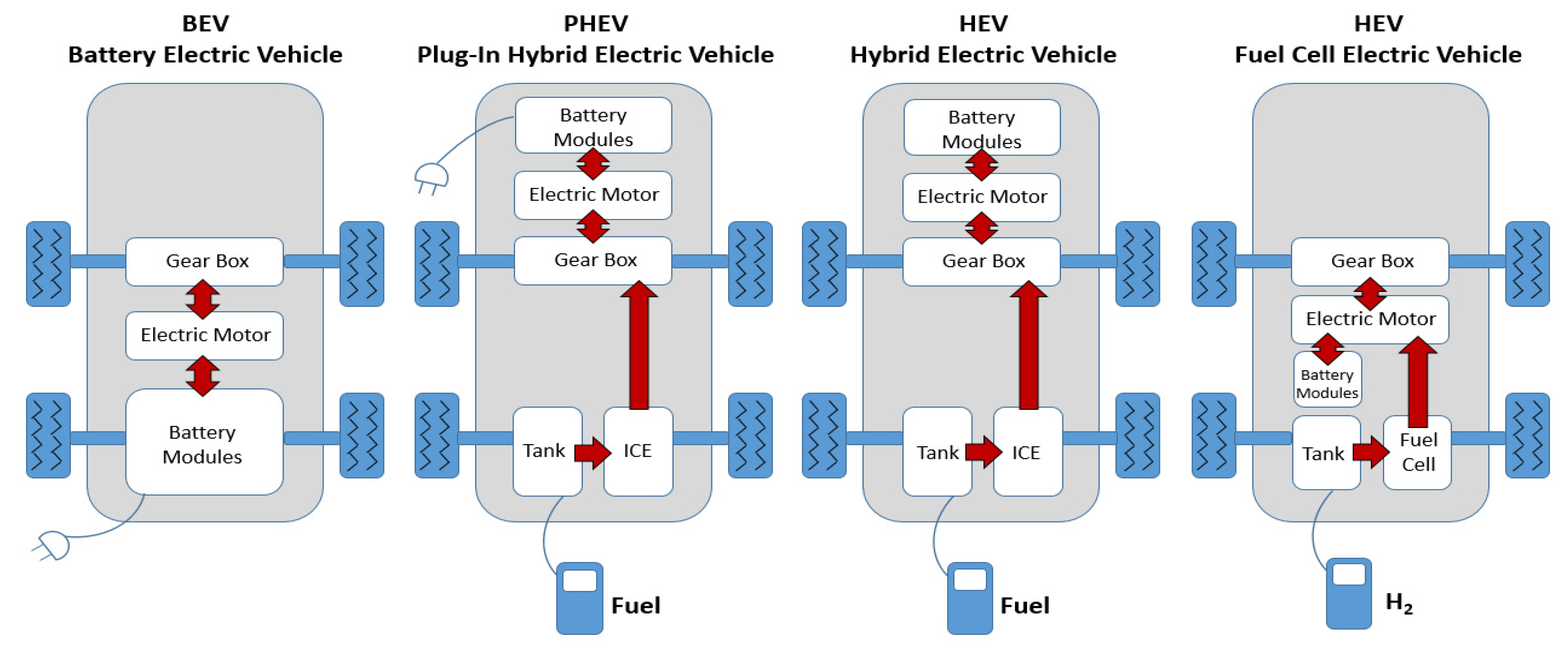
As shown in Figure 1, FCVs are very similar to hybrid or plug-in hybrid electric vehicles in terms of operation [3]. In fact, hybrid electric vehicles are equipped with an internal combustion engine (ICE), its related fuel tank, and battery modules. FCVs instead replace the ICE with a fuel cell stack and its pressurized hydrogen tank. Like internal combustion engines, they make power by using fuel from the tank (pressurized hydrogen gas). In a process that resembles what happens in a battery, in a fuel cell (FC), the hydrogen reacts with oxygen from the air to release electricity, which is used to power the electric motor [4]. In fact, the hydrogen energy density is much higher than that of the best traction batteries, guaranteeing to the FCVs good performance in terms of range [5]. However, FC stacks are characterized by a specific power that is not very high, unidirectional energy flow (i.e., they cannot recover braking energy), and slow dynamics with a reduced lifetime when they are subjected to fast power transients [5,6]. A lithium battery (Li-B) can be used as an auxiliary energy source in order to handle the power transients, recover braking energy, downsize the FC stack, extend its lifetime, and reduce its cost [7]. Thus, an FC-based propulsion system consists of a hybrid ESS (H-ESS) composed of an FC stack, an Li-B-based auxiliary energy source, and an electric powertrain [6,7].
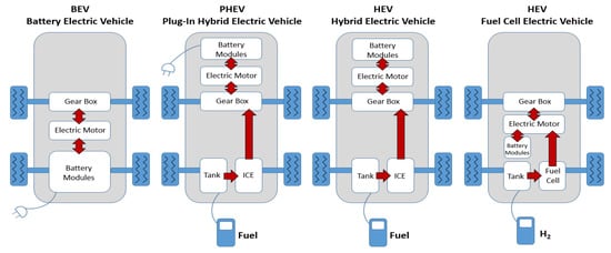
Figure 1.
Types of commercially available EVs today.
Given the dynamic performance of the FCV, fuel consumption is an important performance indicator of the FCV propulsion system affecting the driving range, as the possibilities to carry abundant quantities of hydrogen onboard are limited and expensive [8,9]. Assuming reduction in fuel consumption as the goal, the design procedure of an H-ESS for FCVs consists of finding the sizes of the FC stack and Li-B modules reducing fuel consumption under the condition that the specified driving cycle is feasible. The fuel consumption also depends on how the H-ESS is managed. This is defined by the power split control, which computes the amount of power that the FC stack and Li-B modules have to provide in order to satisfy the power demand of the FCV propulsion system.
The power split strategy significantly affects the component size of the FCV H-ESS, and thus it is necessary to take it into account in the H-ESS sizing methodology in order to obtain more accurate and optimized sizing results [10,11].
1.1. Bibliographic Survey
The bibliographic survey suggests that the design and control of H-ESSs are addressed by using different approaches [8,9,10,11,12,13,14,15,16,17,18,19,20,21,22,23,24]. In particular, the sizing optimization of the FC and supercapacitor and an effective energy management strategy between the FC, Li-B, and supercapacitor are approached and discussed in [8,9], respectively. The energy management control of FCVs aimed at minimizing the fuel consumption is proposed in [10], whereas a power split methodology considering FC longevity is presented in [11]. In [12], the effect of the stack and battery sizes on hydrogen consumption is investigated for an existing FC hybrid distribution truck, while [13] proposes a power split methodology by using distance-based optimized speed and state of charge (SoC) profiles. In [14], Dépature et al. tested a multi-source system composed of fuel cells and supercapacitors, implementing a real-time back-stepping control. In [15], an effective energy management strategy is formulated for multiple sources to optimize fuel consumption, whereas [16] approached the power split problem by using a fuzzy logic-based method. In [17], the authors analyzed the powertrain design of a hybrid electric vehicle which is powered by FC, Li-B, and photovoltaic panels. In [18], an optimized real-time energy management strategy for power split hybrid electric vehicles is proposed. Moreover, in [19], a new methodology based on the statistical description of driving cycles is applied to size the energy source of an FC-based collection truck, whereas in [20], an energy management approach based on specific fuel consumption due to load shifting is proposed. In [21], the energy management strategy of an FCV is implemented by using model-based reinforcement learning with a data-driven model update, whereas the experimental validation of a power split strategy of an FCV is proposed in [22]. Some other papers deal with efficient power conversion technologies. In particular, in [23], a power conversion topology based on a hybrid modulation technique is proposed which is aimed at minimizing the switching losses in the inverter, whereas in [24], the model of an FCV drive train is introduced to implement model predictive control for power converters.
The proposed bibliographic survey shows a lack of research on sizing methodologies for H-ESS taking into account the power split strategy for reducing the overall weight of the FCV and the fuel consumption. Moreover, existing power split methods do not consider accurate electrical models of FC stacks and battery modules in order to estimate their transient dynamic and maximum available power during each time step.
1.2. Innovative Contribution
With this in mind, here, we introduce a joint two-stage sizing procedure for the FC stack and Li-B of an FCV to minimize its fuel consumption. In particular, the proposed approach takes into account the power split strategy for optimizing the sizing of the H-ESS and reducing its weight. In particular, the proposed power split approach takes into account the different technical characteristics of both the FC stack and Li-B modules by defining their lumped resistance. The sizing methodology is composed of the following steps: (1) select a set of driving cycles that the FCV has to be able to implement; (2) for each of them, find the optimal parameters of the power split strategy aimed at maximizing the expected lifetime of the FC stack and Li-B modules; (3) for each driving cycle and each set of optimized parameters for the power split strategy, find the optimal sizing of the FC stack and Li-B modules aimed at minimizing fuel consumption; and (4) find the optimal sizing of the H-ESS component and the parameters’ values of the power split strategy able to satisfy the requirements of all driving cycles. A software simulator implements the electric sub-models of the FCV, and the results obtained using different driving cycles show the effectiveness of the proposed approach.
The remainder of the paper is organized as follows. Section 2 and Section 3 describe the modeling of the FCV powertrain and the proposed power split methodology, respectively. Section 4 presents the procedure, including the power split method, for the sizing of the hybrid ESS. The results of several simulations based on different driving cycles are presented and discussed in Section 5, whereas Section 6 ends the paper with the concluding remarks.
2. Powertrain Architecture and Modeling
In this section, the powertrain architecture and the kinematic model of the EV are presented. Moreover, the electrical sub-models of the power converters, the fuel cell stack, and the battery modules are introduced.
2.1. EV Kinematic Model
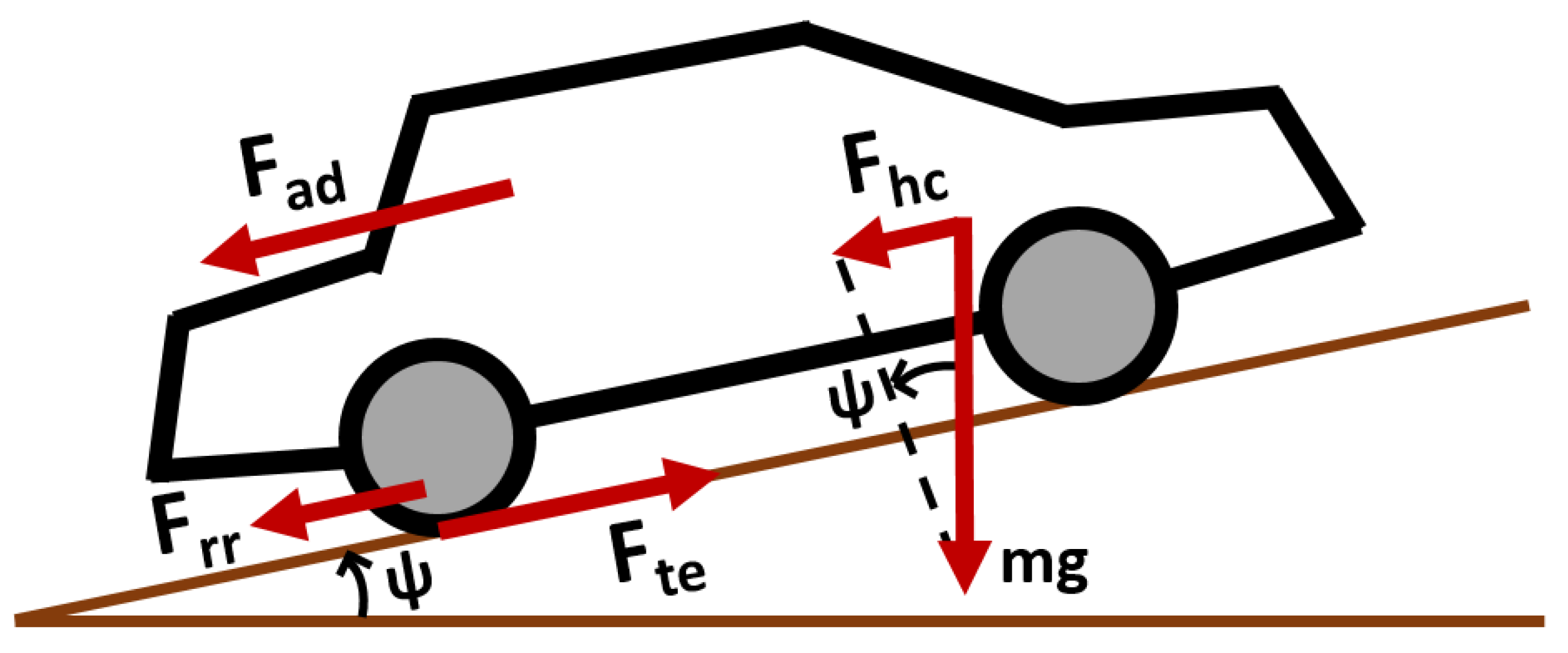
The force propelling the vehicle forward (i.e., the tractive effort Fte) has to accomplish the rolling resistance Frr, the aerodynamic drag Fad, the force needed to overcome the component of the EV weight acting down a slope Fhc and the force to accelerate the vehicle Facc. Thus, the tractive effort is the sum of all these forces, as shown in Figure 2, and it can be expressed as follows [25,26]:
where m is total vehicle mass (driver, passenger, and payload), g is the gravitational acceleration, Crr is the coefficient of rolling resistance, and ψ is the angle of the road slope. Following this, ρ is the density of air, Cd is the aerodynamic drag coefficient, Af is the vehicle frontal area, and v is the speed of the vehicle. Finally, I is the moment of inertia of the motor, G is the gear ratio, r is the radius of the tires, and ηg is the gearbox efficiency.

Figure 2.
Review of the main forces acting on a vehicle.
By starting from an imposed speed cycle, it is possible to derive the mechanical power at the wheels. Then, the total electric power required by the overall electric powertrain PDC-link is computed by going back through the efficiencies of all the vehicle components, and this is given by
where PAUX is the average power required by the auxiliary systems, such as the onboard electronic systems, horn supply, headlights, signal lights, air conditioning, and fuel cell auxiliary systems, and ηi represents the inverter constant efficiencies, whereas ηm is the induction motor efficiency, which is expressed as follows:
In Equation (3), T and ω are the motor torque and angular speed, respectively. The term kcT2 describes the copper losses caused by the electrical resistance of the motor wires, kiω represents the iron losses, taking into account both hysteresis and eddy current effects in the iron rotor, and kwω3 represents the windage losses due to the friction and wind resistance of the rotor [25]. The values of the coefficients kc, ki, and kw can be found by regression using measured values of efficiency or with the manufacturer datasheet.
2.2. EV Architecture and DC/DC Converters Model
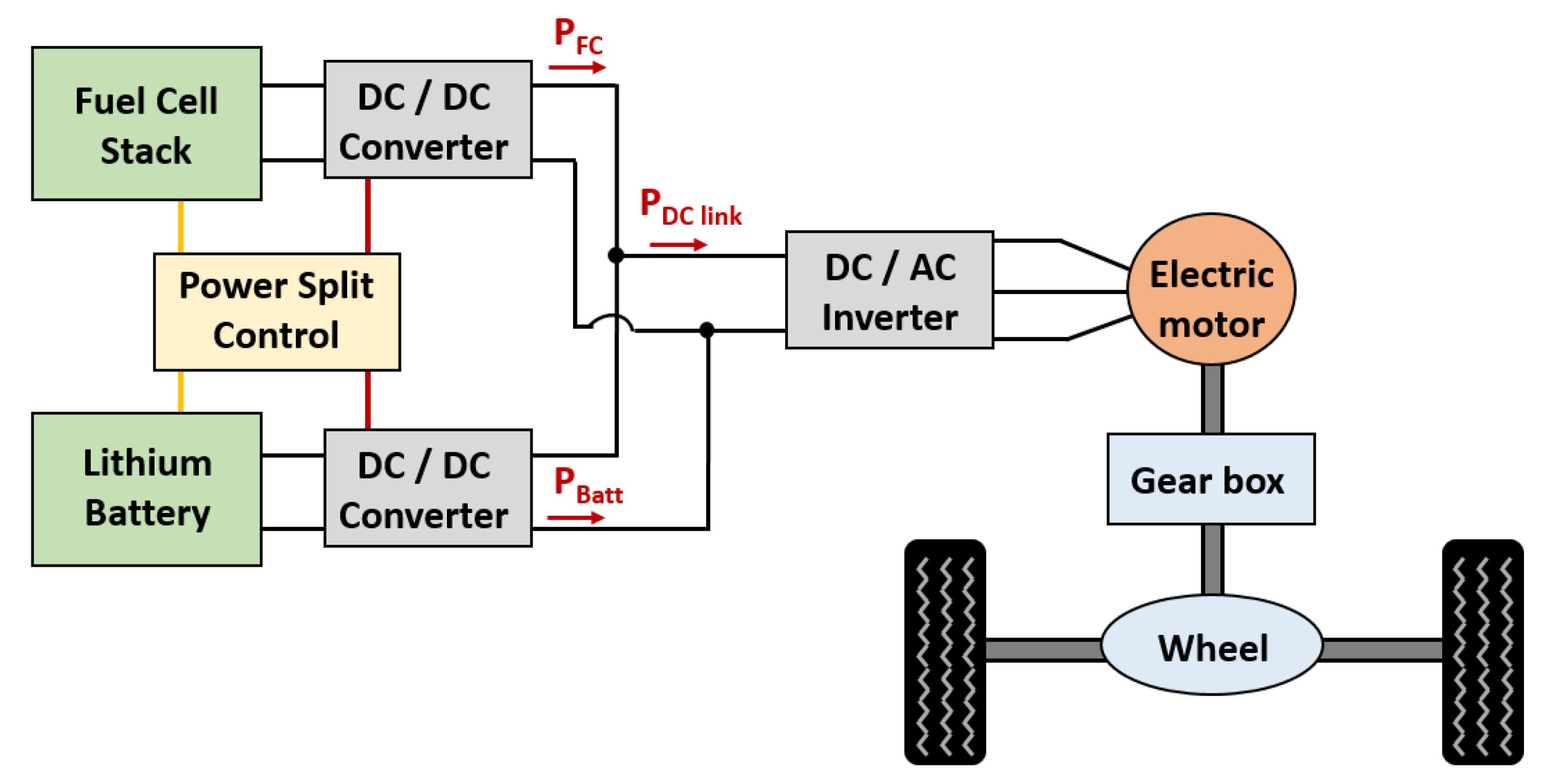
Figure 3 illustrates the overall system configuration of a fuel cell hybrid electric vehicle. Usually, a transmission system is not necessary because the electric motor exhibits good torque performance in a low-speed operational range, and only a fixed-ratio differential is used to reduce high motor speeds. There are four key components in the system: (1) the powertrain, consisting of the DC/AC inverter, electric motor, gearbox, and wheels; (2) the fuel cell stack; (3) the Li-B modules acting as an auxiliary energy storage system; and (4) the DC/DC converters interfacing the stack and the modules to the dc bus voltage (DC-link).

Figure 3.
System structure of the fuel cell hybrid electric vehicle.
Therefore, the power flow at the DC-link is given by
where PFC is the power value supplied by the fuel cell and PBatt is the power value stored or supplied by the Li-B modules. We compute the value of the current supplied by the hybrid ESS as the ratio of the DC-link electric power (absorbed or generated by the powertrain) and the DC-link voltage VDC-link. We compute the value of the input/output current of the DC-DC converter by equating its input and output power and taking into account a constant efficiency value:
The value ηDCDC represents the efficiency of the unidirectional and the bidirectional DC-DC power converter interfacing the FC stack and the Li-B modules to the DC-link, respectively.
2.3. Fuel Cell Model
The considered fuel cell circuit model is based on the following assumptions [27]:
- The average stack temperature is assumed to be constant due to the slower dynamics of the stack temperature;
- All gases supplied to the FC obey the ideal gas law;
- The fuel cell is fed with a continuous supply of reactants to allow operating conditions at a sufficiently high flow rate;
- The mole fractions of the inlet reactants are assumed to be constant to build the FC stack model.
Based on these assumptions, the output fuel cell voltage VFC is defined in [27] as a function of the reactant partial pressures and the fuel cell temperature T (K) and current IFC as follows:
where dT is the time step, E is the thermodynamic potential of the cell based on the Nernst equation, and Rohm describes the ohmic voltage drop from the resistances of proton flow in the electrolyte, which are given by the following:
where E0 is the electromotive force at standard pressure, R is the universal gas constant (8.134 J/moL∙K), α is the charge transfer coefficient, and F is the Faraday constant (96,487 C). PH2, PO2, and PH2O are the partial pressures of hydrogen, oxygen, and steam, respectively, whereas R0 is a constant resistance value, and ϑ is a coefficient describing the variation of Rohm changing the fuel cell current.
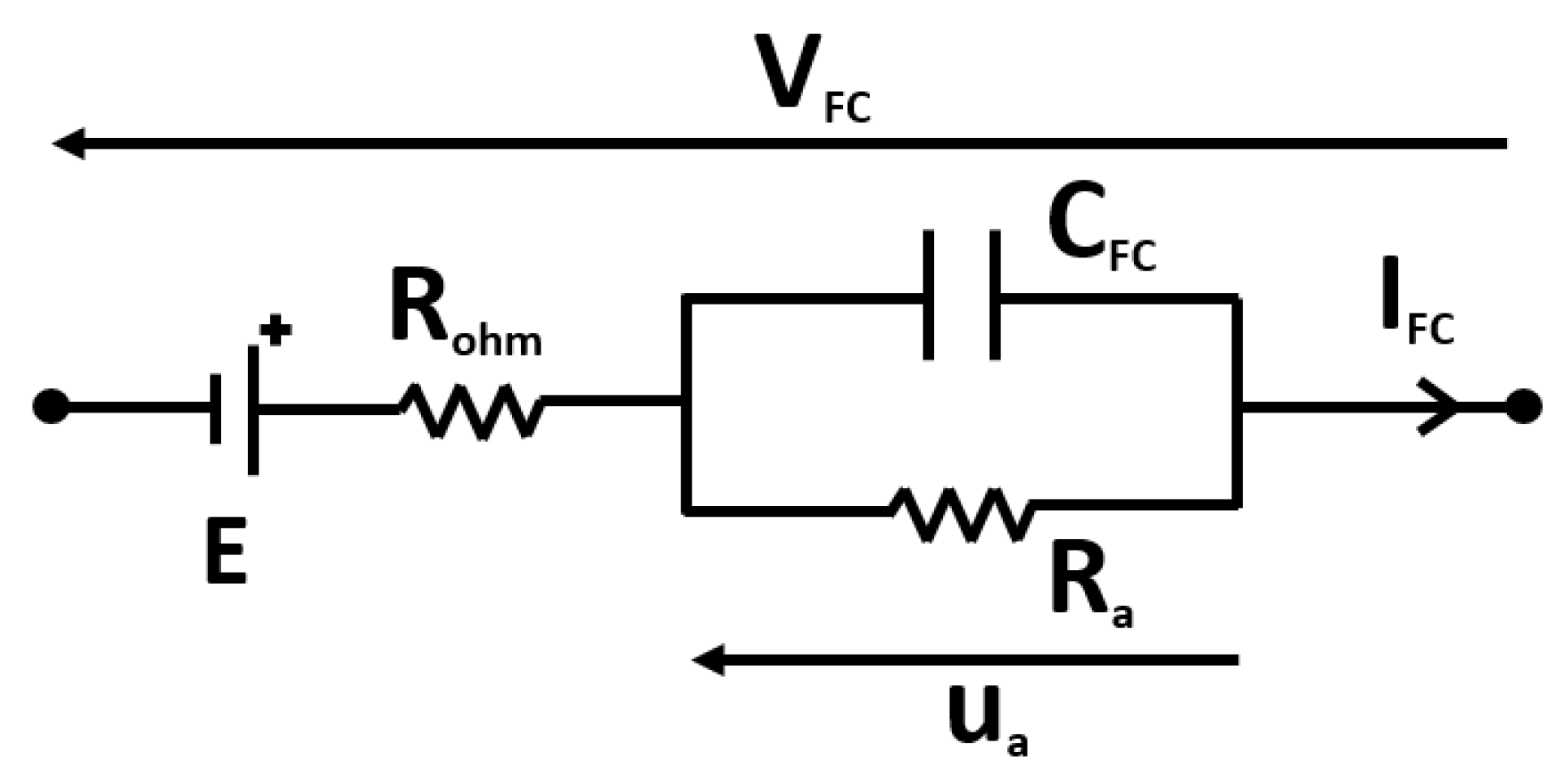
For modeling the fuel cell, a first-order dynamic model based on the effect of the double-layer charging capacitance CFC is considered [27]. CFC describes the electric field created on the electrode–electrolyte interface due to the chemical reaction between protons and electrons, which stores the electrical charge and energy. By defining Ra as the sum of the activation overvoltage resistance Ract and the concentration resistance Rcon, the voltage drop across Ra will be ua, as shown in the general equivalent circuit depicted in Figure 4. Ract describes the voltage loss due to the rate of reactions on the surface of the electrodes, whereas Rcon represents the voltage loss due to the reduction in the concentration of the gases, and their equations are given by
where iFC is the FC current density computed by dividing the IFC into the FC active area AFC, in is the internal current density, and i0 is the exchange current density, whereas m1 and m2 are the constants in the mass transfer voltage, and they are equal to 2.11 × 10⁻⁵ V and 8 × 10⁻³ cm∙mA−1, respectively.

Figure 4.
First-order electrical model of a fuel cell.
2.4. Lithium Battery Model
The four equations describing the first-order equivalent circuit of Li-B cells are reported in Equation (9) and depicted in Figure 5. In more detail, an ideal voltage source represents the open-circuit voltage (OCV), depending on the battery SoC, and the series resistor Rint represents the internal resistance, whereas rd and Cd are the RC parallel circuit describing the charge transfer and double layer capacity, respectively [25,26]. Specifically, the first equation represents Kirchhoff’s voltage law, while the second one is the n-polynomial relation between OCV and SoCBATT. The third equation models the SoC update law, and finally, the last equation is the differential one describing the RC parallel circuit:
where ud(t) is the rdCd parallel circuit voltage, dT is the time step, β0 … βn are interpolation coefficients, and CBATT (kWh) is the battery capacity.
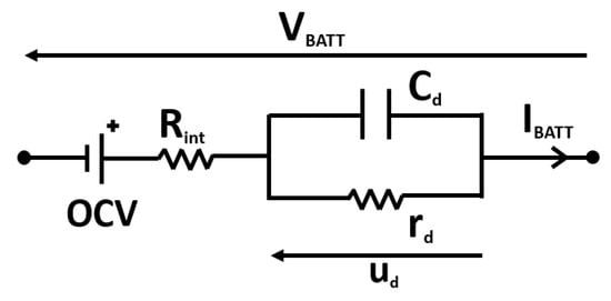
Figure 5.
First-order electrical model of a Li-B cell.
3. Power Split Control
The proposed power split approach is based on the estimation of the lumped resistance for the FC stack and Li-B modules in order to estimate their maximum allowable power variation for a given time interval. Therefore, the algorithm splits the powertrain demand between the FC and the Li-B according to a linear relationship and while taking into account the load curve.
The lumped resistance is the magnitude of the impedance of the FC or Li-B concerning charge or discharge reference current during a fixed time interval [28]. The initial-voltage V1 and the end voltage V2 during the pulse current must be known.
In Figure 6, the terminal voltages are measured by applying a pulse discharge and charge current IP from t1 to t2 for the FC stack or Li-B modules [28]. Therefore, the lumped resistance is calculated from Equation (10).
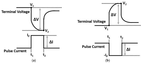
Figure 6.
(a) Terminal voltage response to a pulse discharging current. (b) Terminal voltage response to a pulse charging current.
The voltage values at t1 and t2 can be obtained using the electrical models described in the previous section. We assume the maximum pulse current given by the manufacturer datasheet, as the IP value, is applied at t1. The maximum charge/discharge current variation from t to t + dT ( and , respectively) ensuring the FC or Li-B operates within its safety areas, is computed as follows:
where V1(t) is the current terminal voltage according to the charging/discharging current at time t, whereas Vmin and Vmax denote the minimum and maximum voltages for the safe operation of the FC or Li-B. Moreover, the coefficient ζ is between 0 and 1 and reduces the operating area of the Li-B modules to increase their life span.
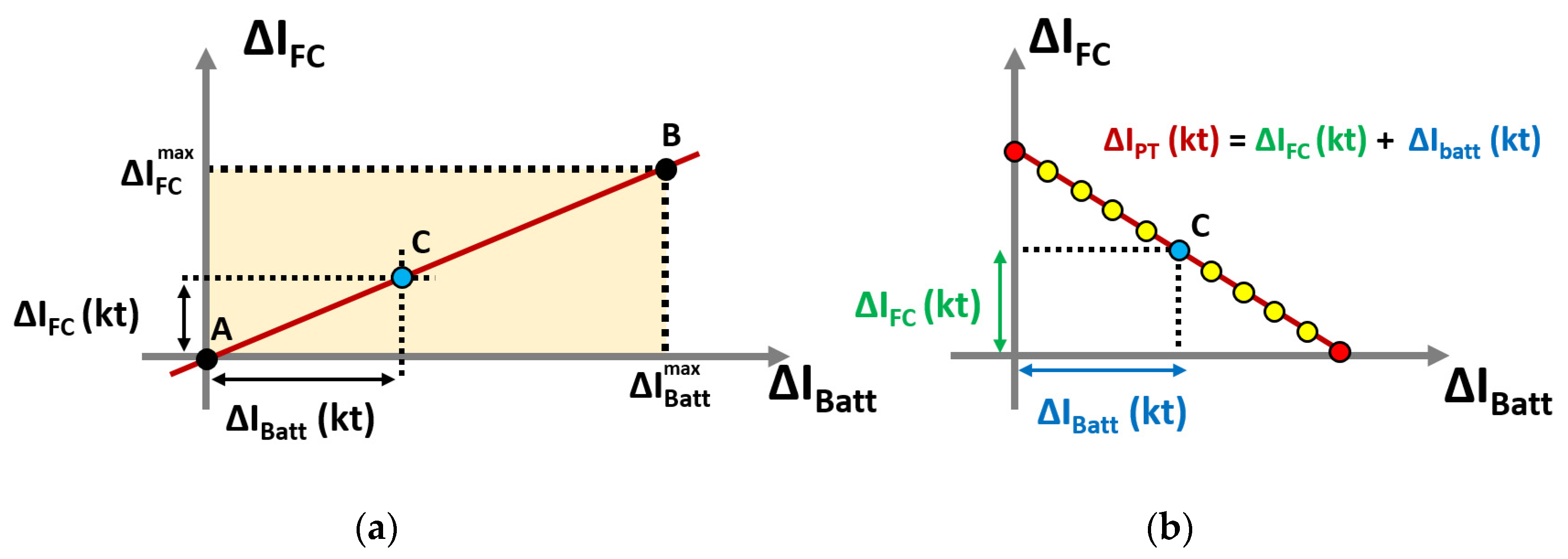
Without loss in generality, Figure 7a shows the dynamic operating area for positive variations of the hybrid ESS. This is defined by the plane including all the admissible FC stack and Li-B current variations in the dT time interval starting from the actual working point. Points A and B identify the zero and maximum values of the current variation for the FC and Li-B , respectively. Hence, it is possible to define a straight line that passes through points A and B updated from time to time according to the current values of and , on which the operating point of the FC and Li-B hybrid ESS lies.

Figure 7.
(a) Linear relationship for power splitting. (b) Load curve for a given value.
Figure 7b instead shows the load curve of the FC and Li-B hybrid ESS at the dT time interval. The red points represent the operating points where the overall powertrain demand is provided only by the FC stack or Li-B modules. The yellow points represent different solutions to the power split algorithm, whereas the blue point C is the intersection between the linear relationship for power splitting and the load curve. Point C is the operating point of the hybrid ESS, and it highlights the power split at the dT time interval between the FC and Li-B for a given demand value of the powertrain current .
In more detail, given a value, the algorithm computes the values of the FC and Li-B current variations ∆IFC and ∆IBatt, respectively, by finding the point of intersection between the straight line defined in Figure 6a and that in Figure 6b (i.e., by solving Equation (12)):
where a(t) and b(t) are the slope and the constant coefficients, respectively, of the straight-line relationship defined by points A and B. The solution of the set in Equation (12) is given by
To avoid the FC being stressed by small variations in the powertrain demand, the described power splitting relationship is applied only if is greater than the minimum value of the powertrain demand . Otherwise, only the Li-B provides the current change according to Equation (14):
It is worth noting that the values are computed in compliance with the Li-B SoC values. For negative values of the powertrain current (i.e., during regenerative braking), the algorithm similarly splits the power up to the FC stack current reaching zero. In such a case, past that point, only the Li-B modules stores the braking energy, taking into account that the FC stack is a not a reversible energy source.
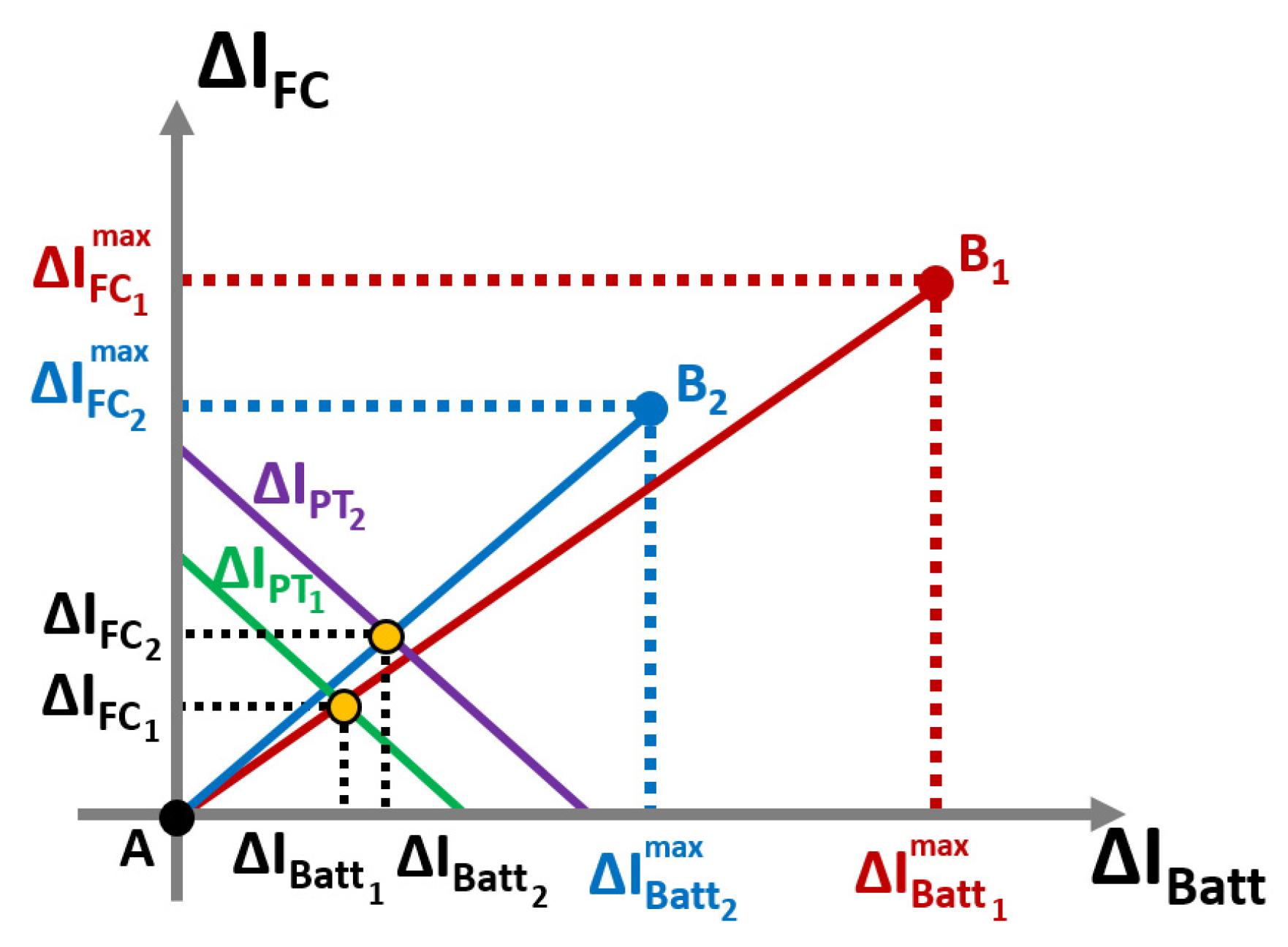
Figure 8 shows the linear relationship for power splitting and the load curve for different values. In particular, green and purple straight lines represent the load curves for and powertrain demand, respectively. Moreover, red and blue straight lines represent the linear relationships for power splitting. Finally, the yellow points represent the FC stack and Li-B modules operating points according to the proposed power split procedure.
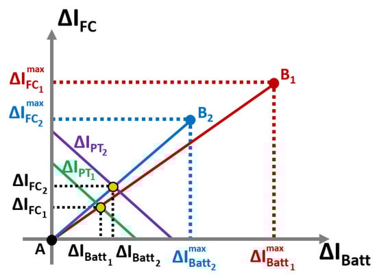
Figure 8.
Intersection between the linear relationship for power splitting and the load curve for different values.
Algorithm 1 shows the pseudocode of the Power Split Algorithm for hybrid ESSs consisting of FC stack and Li-B module in order to clarify each step in detail.
| Algorithm 1: Power split algorithm for hybrid FC stack and Li-B module ESSs. |
| Loop (for each time interval): # check if the powertrain demand is positive or negative If ( > 0) # check if the powertrain demand is lower than the value If () # if 20% < SoC(k) < 100% # compute the power split solutions for FC stack and Li-B modules end # check if the powertrain demand is greater than the value If () # if 20% < SoC(k) < 100% # compute the maximum FC stack and Li-B modules current value # compute the a and b linear coefficient of the power split relationship # compute the power split solutions for FC stack and Li-B modules end # check if the powertrain demand is positive or negative If ( ≤ 0) # check if the FC supplied current is positive If () # if 20% < SoC(k) < 100% # compute the a and b linear coefficient of the power split relationship # compute the power split solutions for FC stack and Li-B modules end # check if the FC supplied current is negative If () # if 20% < SoC(k) < 100% # compute the a and b linear coefficient of the power split relationship # compute the power split solutions for FC stack and Li-B modules end end |
4. Sizing Method for a Hybrid ESS
The proposed sizing method consists of a two-stage optimization procedure. In the first stage, given a preliminary FC stack and the Li-B module sizing, we derive the optimal parameter values of the proposed power split procedure. In the second stage, given the optimal parameter of the power split strategy (obtained in the first stage) instead, the FC stack and the Li-B module sizing are optimized to implement a set of given driving cycles.
4.1. Stage One
The sizing problem yields the optimal sizes of the FC stack and Li-B modules that minimize the fuel consumption necessary to implement a set of given driving cycles. The size of the FC stack is defined by its maximum power PFCmax, whereas both the maximum battery capacity EBmax and power PBmax, which is equal to δ (h−1) times the maximum battery capacity, define the Li-B storage. Therefore, for a given driving cycle, the proposed sizing problem consists of finding the minimum value of the FC stack maximum power and Li-B maximum energy able to minimize the fuel consumption mH2 and the Li-B weight mBatt. Equation (15) reports the proposed objective function, in which the decision variables are assumed to be PFCmax and EBmax:
The objective function in Equation (15) is bound to the following constraints:
The constrains of the sizing problem Z are the δ value associated with the C rate for identifying the maximum Li-B power, the range value at the end of the driving cycle, representing the FCV range in km that the vehicle will cover, and the power required by the powertrain PPT to implement a given speed cycle. Finally, the Li-B SoC is constrained to a minimum and maximum value, while α and β are the weighting coefficients. The hydrogen consumption for the FC stack mH2 is computed through a simulation of the given driving cycles, and it is expressed as follows:
In Equation (17), MH2 is the molar mass of hydrogen (2.01588 g/moL), IFC is the current of the FC stack, F is the Faraday constant (96,487 C), and T is the duration of the reference speed cycle. The proposed sizing problem takes into account the weight of the FC stack and Li-B modules through the following linear relationship:
In Equation (18), we assume that m0 is the initial vehicle weight, including propulsion system components such as the hydrogen tank and auxiliaries, except for the fuel cell stack and battery. The power density of the fuel cell system ρFC, the energy density of the battery ρBatt, and the weight of the passengers and payload mpayload define the additional weight.
4.2. Stage Two
The sizing problem Z depends on the power split strategy such that the optimization problem Q finds the optimal values of the following parameters related to the proposed power split method: ζFC, which is the ζ value for the FC stack, ζBatt, which is the ζ value for the Li-B modules, and . To solve the Q problem, a complete kinematic and electromechanical simulation of the FCV implementing a given driving cycle is required. Therefore, the objective function for the Q problem is aimed at maximizing the life span of the FC stack and Li-B modules, and it is reported in Equation (19):
In Equation (19), the decision variables are ζFC, ζBatt, and , representing the parameter set of the proposed power split strategy. LSFC and LSBatt represent the expected lifetime of the FC stack and the Li-B modules, respectively, whereas γ and θ are weighting coefficients:
Moreover, the constraints in Equation (20) limit the decision variables to their minimum and maximum values.
The US Department of Energy (DoE) defines the End of Life (EoL) of the FC stack as a loss of 10% of the initial performance [29]. Thus, we estimate the lifetime of the FC stack LSFC by using an empirical degradation model:
where ∆P stands for the limited, decreased value of the fuel cell performance from the beginning to the lifetime’s end according to its definition, whereas the denominator represents the FC performance decay rate. Based on [29], the relationship between the fuel cell decay rates and the fuel cell current can be expressed as a quadratic, where c2, c1, and c0 are fitting coefficients. All these parameters are adapted from [30] based on the fuel cell used in this paper [31].
The lifetime of the battery module LSBatt is estimated by using the extended Peukert law, taking into account the discharging current value [32]:
where NLC is the estimated number of charging/discharging cycles provided by the manufacturers, and IBatt(tj) is the Li-B current at time tj, whereas p is the Peukert coefficient, depending on the battery technology [33]. The unknown LSBatt appears inside the M-term sum as well since tM = LSBatt, and thus, the extended Peukert law is solved by using an iterative method, such as the Levenberg–Marquardt method.
It is worth noting that the expected lifetime of the FC stack and Li-B are obtained by repeating the absorbed current with each of the two onboard ESSs until they reach their respective EoLs.
4.3. Solution Algorithm
The block diagram of the solution algorithm for the proposed H-ESS sizing problem is shown in Figure 9. First, one of the driving cycles included in a defined set is selected. Then, given a driving cycle as input, the two-stage procedure for the optimal H-ESS sizing and the selection of the optimal parameters for the power split strategy is performed. In more detail, stage one deals with the joint sizing of the FC stack maximum power and Li-B maximum capacity. At each iteration of stage one, given tentative values of PFCmax and EBmax, the optimal parameters of the power split are computed by minimizing the objective function in Equation (18) in stage two. Given the optimal results of stage two, it is possible to evaluate the objective function in Equation (15), update the tentative values of PFCmax and EBmax, and repeat the same steps until convergence.
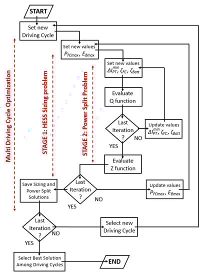
Figure 9.
Block diagram of the H-ESS sizing procedure, including the power split strategy.
The above steps are repeated until the optimal sizing of the H-ESS and its related parameters of the power split strategy are obtained for each driving cycle within the given set. To find the design solution that fits the requirements of each driving cycle, we selected the sizing solution characterized by the maximum value of both the FC stack and Li-B capacity among each found sizing solution. If the sizing solution with maximum value of both the FC stack and Li-B capacity did not exist, we identified the two sizing solutions characterized by the maximum value of the FC stack and the maximum value of the Li-B capacity, respectively. Thus, the design solution between these two is obtained by selecting the one that allows for obtaining the best performance in terms of fuel consumption, even if the peak power that the H-ESS can supply is slightly penalized.
The Z problem is nonlinear and requires solution of the Q problem at each iteration, given the values of the decision variables. For these reasons, it is not possible to derive a closed-form expression. Moreover, the entire solution space is relatively small because the nominal sizes of the FC stack and Li-B commercially available are limited to a few discrete values. Thus, the Z problem is classified as Integer Nonlinear Programming (INLP), and an exhaustive search of the solution space is performed to find the optimal set of the design parameters (PFCmin and EBmin).
The Q problem is also nonlinear and requires a complete simulation based on a given driving cycle. It is not possible to derive a closed-form expression even for the Q problem. The decision variables are assumed to be continuous, and then the Q problem is classified as Nonlinear Programming (NLP). Therefore, we used a heuristic algorithm such as Particle Swarm Optimization (PSO) for solving the problem in stage two, reducing the computing time. We compared the results obtained by using the proposed PSO-based solution algorithm to those of a brute-force search in order to validate the results.
An FCV simulator computes the fuel consumption by repeating the reference speed cycle until the minimum range required by the FCV specifications. We used a software simulator of the FC vehicle with the H-ESS, obtained by implementing the electric models introduced in Section 2 and based on the “quasi-static” backward-looking method [12,26]. In each time step, the mechanical power required by the FCV to satisfy the speed cycle is determined at the wheel level. The electric power provided by the FC stack and Li-B is computed by considering the efficiency of each electrical and mechanical powertrain component and the power split control.
5. Simulation Framework
In order to prove the effectiveness of the proposed methodology, we developed a software simulator coded in Matlab™ by implementing the models and algorithms introduced in the previous sections. Moreover, different sizing results according to different power split strategies are compared and discussed.
5.1. Case Study
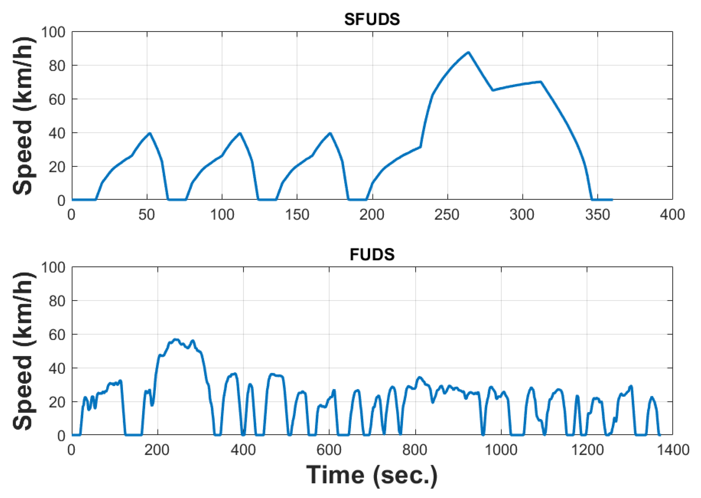
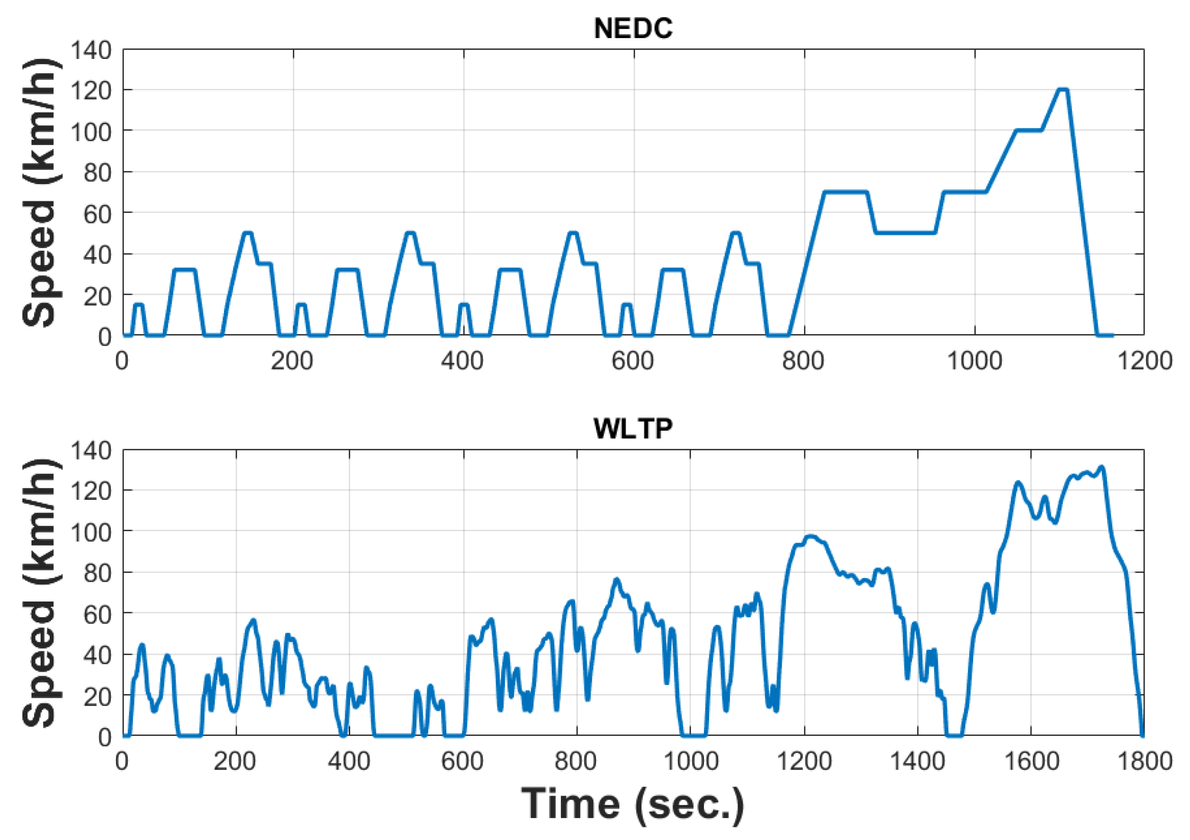
We assumed an FC test vehicle had the characteristics of a conventional urban vehicle summarized in Table 1 and Table 2. We used the European and US standard driving cycles, depicted in Figure 10 and Figure 11, in order to simulate real driving conditions [34]. The federal urban driving schedule (FUDS) and the simplified one (SFUDS) are used for emission testing by the United States Environmental Protection Agency, while the European Commission suggests the use of the new European driving cycle (NEDC) and the Worldwide Harmonized Light Vehicles Test Procedure (WLTP) for testing the performance of battery-based EVs or FCVs in terms of range [35].

Table 1.
FC test vehicle parameters.
Table 2.
Electric motor parameters.
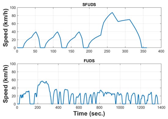
Figure 10.
SFUDS (top) and FUDS (bottom).
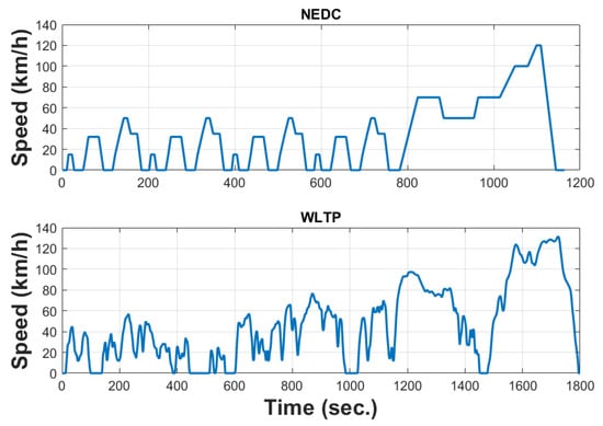
Figure 11.
NEDC (top) and WLTP (bottom).
According to the FCV specifications, the H-ESS has to guarantee more than 750 km of range and dynamic behavior in terms of power supplied to the propulsion system that is able to implement a driving cycle set composed by the SFUDS, FUDS, NEDC, and WLTP. For the FCV understudy, the power density of the FC stack was taken to be 130 W/kg, and the Li-B energy density was taken to be 120 Wh/kg [12]. A fixed payload of 150 kg and 2 passengers (180 kg) were assumed. Moreover, we also assumed a mass of 5 kg of hydrogen stored in a high-pressure tank of about 90 kg [36].
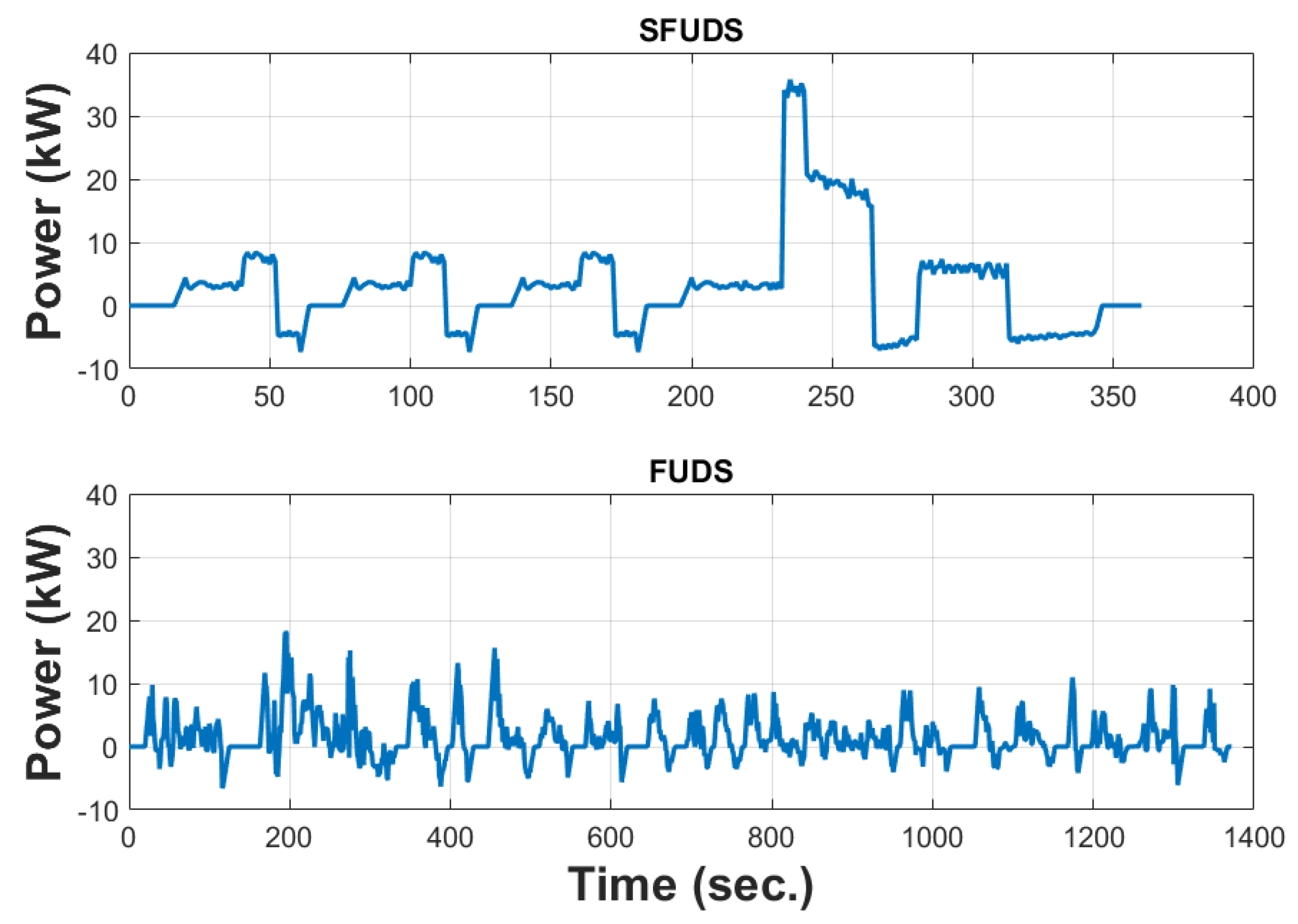
Starting from the FCV’s initial weight, in Figure 12 and Figure 13, we show the electric power supplied from the H-ESS to the DC-link when the FC test vehicle followed the various driving cycles. In particular, while the NEDC and SFUD are characterized by several constant acceleration and speed phases, the FUDS and WLTP continuously present fast variations in speed (i.e., electric power absorbed by DC-link), requiring good performance in terms of H-ESS dynamics.

Figure 12.
Electric power required by SFUDS (top) and FUDS (bottom).
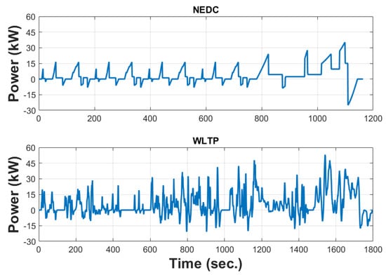
Figure 13.
Electric power required by NEDC (top) and WLTP (bottom).
5.2. Numerical Results
The fuel consumption of the FCV depends on the H-ESS weight, the driving cycle, and the power split algorithm. Thus, we performed several simulations to test the proposed sizing algorithm by using several driving cycles and three different power split strategies. The first one (Psplit1) was based on the FC stack and Li-B lumped resistances and is described in Section 3. The second one (Psplit2) split the power required by the propulsion system during the traction phase according to a sliding average of the FC stack power supplied in the previous time steps, which were assumed to be 0.1 s. The Li-B modules instead stored the entire electric power generated during the regenerative braking. The third one was based on a fuzzy logic methodology [37]. In detail, in this method, the propulsion power demand and the SoC of the Li-B modules were fuzzed by using triangular membership functions. According to the empirical rules applied to the fuzzy set, we calculated the output weight coefficient representing the percentage of the power assigned to the Li-B modules.
Table 3, Table 4 and Table 5 summarize the FC stack and Li-B module designs for the different driving cycles and power split strategies. It is worth noting that it was assumed δ = 1 for the following design solutions, and thus the obtained sizing of the Li-B modules was characterized by much more energy than that required due to the required power constraint. In particular, for the NEDC and WLTP driving cycles, the required power to recover braking energy was particularly high (25 kW and 20 kW, respectively), and the capacity of the Li-B modules was oversized.
Table 3.
H-ESS design solutions (Psplit1): δ = 1.
Table 4.
H-ESS design solutions (Psplit2): δ = 1.
Table 5.
H-ESS design solutions (Psplit3): δ = 1.
In detail, the performances of the Psplit1 algorithm were strictly dependent on the width of the sliding average window. The more this value increased, the more the current of the FC stack was close to being constant. However, the sizing of the Li-B grew accordingly. In this paper, we selected a window width equal to 100, representing a good trade-off between the FC stack current dynamic and Li-B module sizing. By using the Psplit3 method, we were able to better estimate the FC maximum power (using the lumped resistance), and the sizing of the battery modules was significantly reduced compared with Psplit2.
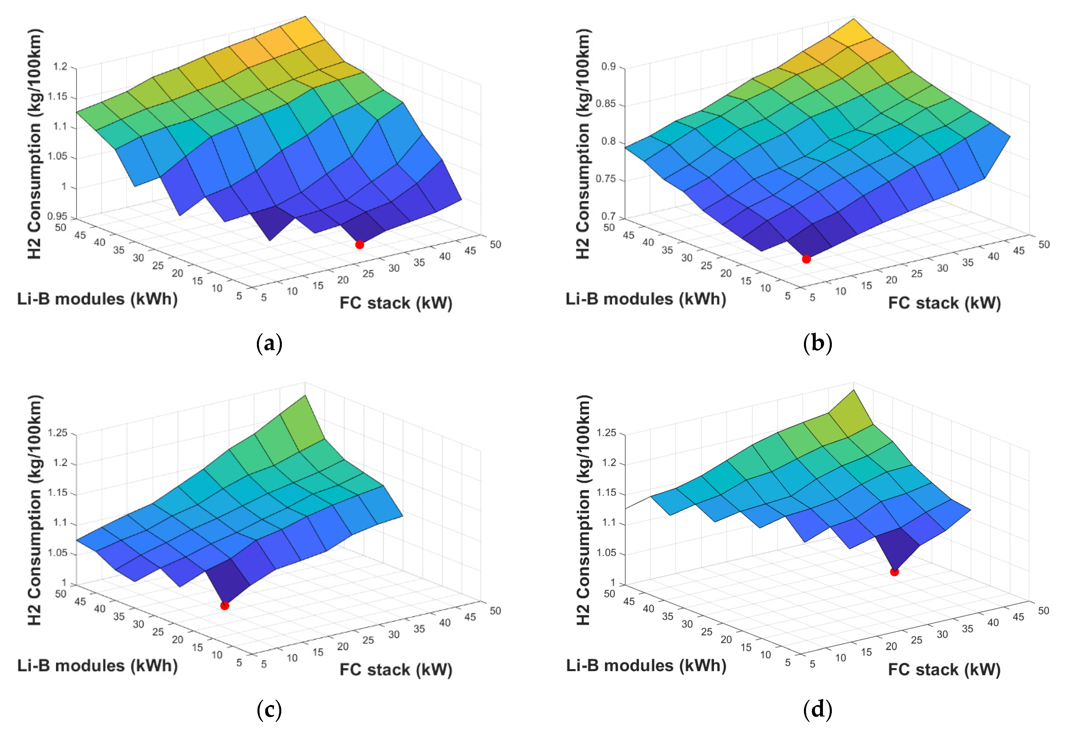
The obtained results show that the H-ESS designed according to the proposed approach could match the power demand of the powertrain. In particular, Figure 14, Figure 15 and Figure 16 show the fuel consumption for different sizes of FC stacks and Li-B modules by imposing the SFUDS, FUDS, NEDC, and WLTP driving cycles and the Psplit1, Psplit2, and Psplit3 algorithms, respectively. We assumed a step size of 5 kW for both the FC stack and the Li-B modules.

Figure 14.
Fuel consumption of the FCV (Psplit1: δ = 1): (a) SFUDS, (b) FUDS, (c) NEDC, and (d) WLTP.
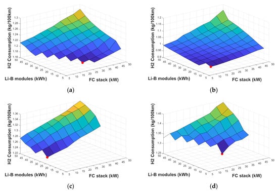
Figure 15.
Fuel consumption of the FCV (Psplit2: δ = 1): (a) SFUDS, (b) FUDS, (c) NEDC, and (d) WLTP.
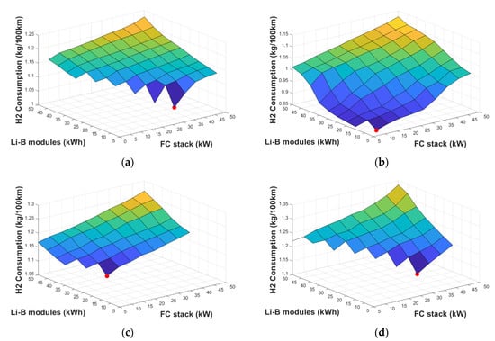
Figure 16.
Fuel consumption of the FCV (Psplit3: δ = 1): (a) SFUDS, (b) FUDS, (c) NEDC, and (d) WLTP.
It is worth noting that the NEDC and SFUDS fuel consumption were very similar, but FUDS is an urban driving cycle instead, and it is characterized by a low peak value but frequent variations in speed and presents the lower value of fuel consumption. The WLTP driving cycle is characterized by the highest fuel consumption. Moreover, the WLTP and NEDC driving cycles are characterized by high values of braking power, and it requires large Li-B module sizing. Therefore, the sizing solution space is reduced.
The best performance of the Psplit1 control allowed for reducing the weight of the Li-B modules and thus reducing the fuel consumption of the FCV by about 21% compared with the Psplit2 control and about 9% compared with the Psplit3 control. It is worth noting that FUDS and WLTP required larger battery sizing due to their fast speed variations and therefore showed a slightly higher fuel consumption compared with the SFUDS and NEDC.
The methodology described in Section 4.3 allowed for obtaining the FC stack and Li-B module sizing by taking into account the entire set of driving cycles. In particular, by considering the Psplit1 strategy, we obtained an FC stack of 35 kW and Li-B of 20 kWh. Moreover, an FC stack of 30 kW and Li-B of 24 kWh were obtained by assuming Psplit2, whereas an FC stack of 33 kW and Li-B of 22 kWh were obtained with Psplit3.
The effect of the δ coefficient on the sizing procedure is highlighted in Table 6, Table 7 and Table 8 by varying the driving cycle and the power split strategy. Greater values of the δ coefficient mean the assumption of Li-B modules with a higher specific power. Thus, in the condition of the same available power, the battery weight was reduced, and consequently, so was the fuel consumption. By increasing the δ value, the performance in terms of fuel consumption improved for the three different power split strategies as the weight of the Li-B modules was reduced. However, the Psplit1 showed the best performance, because it was able to optimize the use of the FC stack by minimizing the sizing of the Li-B modules and therefore the related weight.
Table 6.
Effect of δ on the sizing procedure (Psplit1).
Table 7.
Effect of δ on the sizing procedure (Psplit2).
Table 8.
Effect of δ on the sizing procedure (Psplit3).
Table 6, Table 7 and Table 8 show that for each driving cycle, the Li-B module sizing was reduced in terms of required energy as the δ value increased. However, this reduction trend stopped when the minimum energy required by the Li-B modules was reached.
The proposed sizing methodology was compared with a separate FC stack and Li-B module sizing method. In particular, the FC stack was sized by considering the maximum value of the average propulsion power, whereas the Li-B modules were sized by considering the maximum difference between the propulsion’s required power and the FC stack’s rated power while assuming δ = 1.
The obtained results show that the FC stack capability was underestimated, and consequently, the Li-B modules were overestimated. For such reasons, the weight of the H-ESS was increased compared with the proposed methodology, and therefore, even the fuel consumption increased.
In particular, by considering the separate sizing method and Psplit3 strategy, the obtained sizing for the H-ESS among the set of driving cycles resulted in an increased weight of about 18% compared with the proposed method and increased fuel consumption by about 12%.
Finally, Table 9, Table 10 and Table 11 show the expected lifetime of the FC stack and Li-B modules (δ = 1) by assuming different power split strategies and considering different driving cycles. In more detail, FUDS and WLTP were the most stressing cycles for both the FC stack and Li-B modules. In fact, they allowed lower lifetimes compared with those of SFUDS and NEDC. Once again, the Psplit1 strategy was able to maximize the expected lifetime by minimizing the sizing at the same time and then reducing the fuel consumption of the FCV. It is worth noting that the expected lifetime of the Li-B modules in the case of δ = 1 was higher than that obtained for δ = 3.
Table 9.
Comparison of expected lifetime (Psplit1: δ = 1).
Table 10.
Comparison of expected lifetime (Psplit2: δ = 1).
Table 11.
Comparison of expected lifetime (Psplit3: δ = 1).
The FUDS driving cycle allowed for obtaining the best performances in terms of the expected lifetime of both the FC stack and Li-B modules. Although they were quite similar, the SFUDS and NEDC driving cycles showed different performances. In fact, the SFUDS required a larger size for the FC stack, and its aging results were faster, whereas the NEDC required a larger size for the Li-B modules, and their aging results were faster. The WLTP driving cycle required slightly larger sizing of the FC stack than Li-B modules, and then their aging was slightly faster. The comparison in terms of an expected lifetime according to the power split algorithm followed, in general, the behavior of the performance in terms of fuel consumption.
Although in this paper experimental test activities were not carried out for validating the outputs of the numerical simulations, the obtained results were consistent with those obtained during the experimental measuring activities conducted, for example, in [29,30]. In fact, in these research works, it is stated that the expected lifetime of Proton Exchange Membrane Fuel Cells (PEMFCs) can be assumed to be around 2000–3000 h for automotive applications.
6. Conclusions
This paper proposes a suitable procedure for the joint sizing of FC stacks and Li-B modules as an H-ESS for FCVs, taking into account the power split strategy. The electric models of the FCV propulsion system, FC stack, and Li-B modules were presented and implemented in a software simulator based on the “quasi-static” backward-looking method. A novel power split approach was proposed by taking into account the different technical characteristics of both the FC stack and Li-B modules, introducing the lumped resistance and being able to maximize the expected lifetime of the H-ESS.
The effectiveness of the proposed joint H-ESS sizing procedure was verified by using numerical simulations implementing several EU and US urban driving cycles and comparing different power split algorithms in terms of fuel consumption. However, the proposed sizing methodology, including the power split strategy, requires complete knowledge of the electrical models for both the FC stack and Li-B modules according to different rated values. Very often, manufacturer datasheets are incomplete or do not provide such data, and this is an obstacle to the applicability of the proposed method. The obtained results show a reduction in the FCV’s fuel consumption up to about 10% compared with that obtained by using existing power split strategies. Moreover, the proposed methodology allows for maximizing the expected lifetime of the FC stack and Li-B modules by minimizing their sizing at the same time. Managerial implications of this research and benefits for FCV manufacturers using the proposed methodology can be summarized as an increase in the vehicle’s performance and a reduction in cost due to the optimized sizing of the H-ESS components.
Future research directions deal with the implementation and testing of the proposed methodology on a real or scaled prototype of the H-ESS. Moreover, the performance in terms of fuel consumption of the FCV could be improved by using an adaptive parameter of the power split algorithm and by implementing an H-ESS energy management strategy that manages the SoC of the Li-B modules while trying to keep it to an intermediate value in order to optimize the Li-B module sizing.
Author Contributions
Conceptualization, G.G. and V.C.; methodology, G.G.; software, G.G.; validation, G.G., V.C. and V.G.; formal analysis, G.G.; investigation, G.G.; resources, G.G. and V.C.; data curation, G.G.; writing—original draft preparation, G.G.; writing—review and editing, G.G. and V.C.; visualization, G.G.; supervision, V.C. and V.G.; project administration, V.G.; funding acquisition, V.C. All authors have read and agreed to the published version of the manuscript.
Funding
This research received no external funding.
Conflicts of Interest
The authors declare no conflict of interest.
References
- United Nations. Report of the Conference of the Parties on Its Twenty-First Session. Available online: chrome-extension://efaidnbmnnnibpcajpcglclefindmkaj/viewer.html?pdfurl=https%3A%2F%2Funfccc.int%2Fresource%2Fdocs%2F2015%2Fcop21%2Feng%2F10.pdf&clen=622273 (accessed on 12 December 2021).
- International Energy Agency (IEA). Global EV Outlook. Available online: https://www.iea.org/reports/global-ev-outlook-2019 (accessed on 4 December 2019).
- The Driven—B. Gaton—The ICE Age Is Over: Why Battery Cars Will Beat Hybrids and Fuel Cells. Available online: https://thedriven.io/2018/11/14/the-ice-age-is-over-why-battery-cars-will-beat-hybrids-and-fuel-cells/ (accessed on 20 December 2021).
- Gao, W. Performance comparison of a fuel cell-battery hybrid powertrain and a fuel cell-ultracapacitor hybrid powertrain. IEEE Trans. Veh. Technol. 2005, 54, 846–855. [Google Scholar] [CrossRef]
- Powercell S3. PowerCellution V Stack Datasheet. Available online: chrome-extension://efaidnbmnnnibpcajpcglclefindmkaj/viewer.html?pdfurl=https%3A%2F%2Fwww.datocms-assets.com%2F36080%2F1636022091-v-stack-v-221.pdf&clen=415644&chunk=true (accessed on 12 December 2021).
- Bauman, J.; Kazerani, M.A. Comparative Study of Fuel-Cell–Battery, Fuel-Cell–Ultracapacitor, and Fuel-Cell–Battery–Ultracapacitor Vehicles. IEEE Trans. Veh. Technol. 2008, 57, 760–769. [Google Scholar] [CrossRef]
- Khaligh, A.; Li, Z. Battery, Ultracapacitor, Fuel Cell, and Hybrid Energy Storage Systems for Electric, Hybrid Electric, Fuel Cell, and Plug-In Hybrid Electric Vehicles: State of the Art. IEEE Trans. Veh. Technol. 2010, 59, 2806–2814. [Google Scholar] [CrossRef]
- Wu, Y.; Gao, H. Optimization of Fuel Cell and Supercapacitor for Fuel-Cell Electric Vehicles. IEEE Trans. Veh. Technol. 2006, 55, 1748–1755. [Google Scholar] [CrossRef]
- Wang, L.; Li, H. Maximum Fuel Economy-Oriented Power Management Design for a Fuel Cell Vehicle Using Battery and Ultracapacitor. IEEE Trans. Ind. Appl. 2010, 46, 1011–1020. [Google Scholar] [CrossRef]
- Geng, B.; Mills, J.K.; Sun, D. Two-Stage Energy Management Control of Fuel Cell Plug-In Hybrid Electric Vehicles Considering Fuel Cell Longevity. IEEE Trans. Veh. Technol. 2012, 61, 498–508. [Google Scholar] [CrossRef]
- Meng, X.; Li, Q.; Zhang, G.; Wang, T.; Chen, W.; Cao, T. A Dual-Mode Energy Management Strategy Considering Fuel Cell Degradation for Energy Consumption and Fuel Cell Efficiency Comprehensive Optimization of Hybrid Vehicle. IEEE Access 2019, 7, 134475–134487. [Google Scholar] [CrossRef]
- Tazelaar, E.; Shen, Y.; Veenhuizen, P.A.; Hofman, T.; van den Bosch, P.P.J. Sizing Stack and battery of a Fuel Cell hybrid distribution Truck. Oil Gas Sci. Technol. 2012, 67, 563–573. [Google Scholar] [CrossRef] [Green Version]
- Lim, H.; Su, W. Hierarchical Energy Management for Power-Split Plug-In HEVs Using Distance-Based Optimized Speed and SOC Profiles. IEEE Trans. Veh. Technol. 2018, 67, 9312–9323. [Google Scholar] [CrossRef]
- Dépature, C.; Lhomme, W.; Sicard, P.; Bouscayrol, A.; Boulon, L. Real-time Backstepping control for fuel cell vehicle using supercapacitors. IEEE Trans. Veh. Technol. 2018, 67, 306–314. [Google Scholar] [CrossRef]
- Gharibeh, H.F.; Yazdankhah, A.S.; Azizian, M.R. Improved energy management for a power-split multi-source fuel cell vehicle based on optimal source sizing and regenerative braking. In Proceedings of the International Conference on Environment and Electrical Engineering, Florence, Italy, 7–10 June 2016; pp. 1–6. [Google Scholar]
- Tao, F.; Zhu, L.; Fu, Z.; Si, P.; Sun, L. Frequency Decoupling-Based Energy Management Strategy for Fuel Cell/Battery/Ultracapacitor Hybrid Vehicle Using Fuzzy Control Method. IEEE Access 2020, 8, 166491–166502. [Google Scholar] [CrossRef]
- Chowdhury, M.S.A.; Al Mamun, K.A.; Rahman, A.M. Modelling and simulation of power system of battery, solar and fuel cell powered Hybrid Electric vehicle. In Proceedings of the International Conference on Electrical Engineering and Information Communication Technology, Dhaka, Bangladesh, 22–24 September 2016; pp. 1–6. [Google Scholar]
- Wu, J.; Ruan, J.; Zhang, N.; Walker, P.D. An Optimized Real-Time Energy Management Strategy for the Power-Split Hybrid Electric Vehicles. IEEE Trans. Control Syst. Technol. 2019, 27, 1194–1202. [Google Scholar] [CrossRef]
- Ravey, A.; Watrin, N.; Blunier, B.; Bouquain, D.; Miraoui, A. Energy-Source-Sizing Methodology for Hybrid Fuel Cell Vehicles Based on Statistical Description of Driving Cycles. IEEE Trans. Veh. Technol. 2011, 60, 4164–4174. [Google Scholar] [CrossRef]
- Sarioglu, İ.L.; Klein, O.P.; Schroder, H.; Kucukay, F. Energy Management for Fuel-Cell Hybrid Vehicles Based on Specific Fuel Consumption Due to Load Shifting. IEEE Trans. Intell. Transp. Syst. 2012, 13, 1772–1781. [Google Scholar] [CrossRef]
- Lee, H.; Cha, S.W. Energy Management Strategy of Fuel Cell Electric Vehicles Using Model-Based Reinforcement Learning with Data-Driven Model Update. IEEE Access 2021, 9, 59244–59254. [Google Scholar] [CrossRef]
- Syed, F.U.; Kuang, M.L.; Czubay, J.; Ying, H. Derivation and Experimental Validation of a Power-Split Hybrid Electric Vehicle Model. IEEE Trans. Veh. Technol. 2006, 55, 1731–1747. [Google Scholar] [CrossRef]
- Prasanna, U.R.; Xuewei, P.; Rathore, A.K.; Rajashekara, K. Propulsion System Architecture and Power Conditioning Topologies for Fuel Cell Vehicles. IEEE Trans. Ind. Appl. 2015, 51, 640–650. [Google Scholar] [CrossRef]
- Sagert, C.; Bender, F.A.; Sawodny, O. Electrical drive train modeling for model predictive control of DC-DC converters in fuel cell vehicles. In Proceedings of the American Control Conference, Chicago, IL, USA, 1–3 July 2015; pp. 4333–4338. [Google Scholar]
- Larminie, J.; Lowry, J. Electric Vehicles Technology Explained, 2nd ed.; John Wiley & Sons Ltd.: Hoboken, NJ, USA, 2012. [Google Scholar]
- Graber, G.; Galdi, V.; Calderaro, V.; Piccolo, A. A Power Split Control Algorithm for Fuel Cell Electric Vehicles using Batteries or Supercapacitors as Auxiliary Storage System. In Proceedings of the International Conference on Clean Electric Power, Santa Margherita Ligure, Italy, 27–29 June 2017; pp. 1–6. [Google Scholar]
- Larminie, J.; Dicks, A. Fuel Cell Systems Explained, 2nd ed.; John Wiley & Sons Ltd.: Hoboken, NJ, USA, 2012. [Google Scholar]
- Lee, S.J.; Kim, J.H.; Lee, J.M.; Cho, B.H. The Maximum Pulse Current Estimation for the Lithium-Ion Battery. In Proceedings of the Applied Power Electronics Conference and Expo, Austin, TX, USA, 24–28 February 2008; pp. 1–6. [Google Scholar]
- Jouin, M.; Bressel, M.; Morando, S.; Gouriveau, R.; Hissel, D.; Pera, M.-C.; Zerhouni, N.; Jemei, S.; Hilairet, M.; Bouamama, B.O. Estimating the end-of-life of PEM fuel cells: Guidelines and metrics. Appl. Energy 2016, 177, 87–97. [Google Scholar] [CrossRef] [Green Version]
- Pei, P.; Chang, Q.; Tang, T. A quick evaluating method for automotive fuel cell lifetime. Int. J. Hydrogen Energy 2008, 33, 3829–3836. [Google Scholar] [CrossRef]
- Li, H.; Chaoui, H.; Gualous, H. Cost Minimization Strategy for Fuel Cell Hybrid Electric Vehicles Considering Power Sources Degradation. IEEE Trans. Veh. Technol. 2020, 69, 12832–12842. [Google Scholar] [CrossRef]
- Liu, D.; Xie, W.; Liao, H.; Peng, Y. An integrated probabilistic approach to lithium-ion battery remaining useful life estimation. IEEE Trans. Instrum. Meas. 2014, 64, 660–670. [Google Scholar]
- Farhadi, M.; Mohammed, O. Energy storage technologies for high-power applications. IEEE Trans. Ind. Appl. 2016, 52, 1953–1961. [Google Scholar] [CrossRef]
- Jeong, N.T.; Yang, S.M.; Kim, K.S.; Wang, M.S.; Kim, H.S.; Suh, M.W. Urban driving cycle for performance evaluation of electric vehicles. Int. J. Automot. Technol. 2016, 17, 145–151. [Google Scholar] [CrossRef]
- Gebisa, A.; Gebresenbet, G.; Gopal, R.; Nallamothu, R.B. Driving Cycles for Estimating Vehicle Emission Levels and Energy Consumption. Future Transp. 2021, 1, 615–638. [Google Scholar] [CrossRef]
- Toyota Mirai Fuel Cell Sedan Priced At $57,500—Specs, Videos. Available online: https://insideevs.com/news/323973/toyota-mirai-fuel-cell-sedan-priced-at-57500-specs-videos/ (accessed on 15 December 2021).
- Lin, H.; Jiang, J.; Wei, S.; Cheng, L. Optimization control for the efficiency of an on-board hybrid energy storage system in tramway based on fuzzy control. In Proceedings of the 11th IEEE International Conference on Compatibility, Power Electronics and Power Engineering, Cadiz, Spain, 4–6 April 2017; pp. 454–459. [Google Scholar]


Publisher’s Note: MDPI stays neutral with regard to jurisdictional claims in published maps and institutional affiliations. |
© 2022 by the authors. Licensee MDPI, Basel, Switzerland. This article is an open access article distributed under the terms and conditions of the Creative Commons Attribution (CC BY) license (https://creativecommons.org/licenses/by/4.0/).