A Convolution Location Method for Multi-Node Scheduling in Wireless Sensor Networks

Abstract

The localization of continuous objects and the scheduling of resources are challenging issues in wireless sensor networks (WSNs). Due to the irregular shape of the continuous target area and the sensor deployment in WSNs, the sensor data are always discrete and sparse, and most network resources are also limited by the node energy. To achieve faster detection and tracking of continuous objects, we propose a convolution-based continuous object localization algorithm (named CCOL). Moreover, we implement the idea of greedy and dynamic programming to design an energy-saving and efficient strategy model (named MSSM) to respond to emergencies caused by multiple continuous targets in most specific WSNs. The simulation experiments demonstrate that CCOL is superior to other localization algorithms in terms of time complexity and execution performance. Furthermore, the feasibility of the multinode scheduling strategy is verified by setting different mobile nodes to respond to the target area in certain green WSNs.

1. Introduction

The application of wireless sensor networks (WSNs) has been promoted and popularized [1] in daily life. WSNs can cover a vast monitoring area [2] and produce a number of data from numerous sensors in a compact manner [3,4]. WSNs usually remotely sense sensitive events or targets to complete tasks of special functions (forest fire warning, environment monitoring, atmospheric pollutant detection, gas leakage monitoring, data collection of smart cities and predictions, etc.) [5].

However, the discreteness of sensing data makes the detection and localization of continuous target(s) a challenging and topical issue. For example, to detect the leakage of toxic gas in real time, deployed sensors sense the context of the concentration of different areas at different times [6]. Due to the unbalanced density and random sampling of sensors, the collected data are usually discontinuous [7], especially for large monitoring areas with a limited number of sensors (monitoring of marine pollutants in the sea or fire monitoring in the forest, etc.). However, the continuous objects in WSNs, such as toxic gases or streams of people, are still maintained in an integrated state, so deviations and errors commonly appear during target detection [8,9]. For these reasons, it is valuable to detect emergencies rapidly and perform some imperative work in many special scenarios of WSNs.

Studies have mainly focused on improving the positioning and accuracy of the edge area for continuous target detection in wireless sensor networks. Most algorithms are based on geometric theories, such as planarization [6], and downsize the target area by analyzing the data of boundary sensor nodes [7]. For instance, Z. Zhou et al. proposed an iterative method to precisely achieve the target edge [10] by repeatedly updating the candidate nodes to boundary nodes.

B. Liu et al. provided an interpolating and inserting virtual sensor node algorithm to improve the accuracy of the continuous object boundary region [11] by reducing the dispersion and insufficiency of boundary data.

Additionally, service scheduling is one of the important approaches for green computing in WSNs. Scheduling is a balanced problem between effectively addressing emergencies of sensitive areas and saving energy during target location. A few low-latency, efficient algorithms and scheduling strategies have been proposed while slightly reducing the performance of WSNs. The sink mobility-aware node scheduling (SMNS) algorithm increases the utilization of network resources [12]. The packet scheduling algorithm improves the performance of WSNs by a protocol [13]. All of these localization methods are based on the topology of the network and the position relationship of the sensors nodes, so that the target location in WSNs depends on the structure of the network and the distribution of sensors [14]. In this paper, we establish a dynamic serving model for emergencies in WSNs and propose a scheme based on multiple mobile nodes to address sensitive areas. The research on these issues is of great significance in some practical applications, including evacuation in densely populated areas, traffic control in emergency situations, personnel control of toxic gas leakage, etc. [15,16].

Considering the irregular and sporadic shape of the continuous objects in WSNs, in this article, we focus on the boundary of the shape of targets and propose a target localization algorithm that used convolution to solve the discontinuity of data corresponding to different grids in wireless sensor networks. Furthermore, we discuss the scheduling strategy of emergency areas in WSNs and give an efficient and speedy multiple mobile node approach. The simulated results demonstrate the feasibility of the scheme. In this essay, our main work and contributions include the following:

(1) Proposing a fast method based on convolution for the positioning of continuous targets in WSNs.

(2) Putting forward a multiple mobile node dispatch model for emergencies in WSNs.

(3) Comparing the results of the algorithm performance and energy consumption of the network nodes and verifying the feasibility of the perspective.

Section 2 introduces the background of the problem and related works. Then, Section 3 explains the theoretical basis of the algorithm and the establishment of the model. The remaining sections elaborate on the core algorithms and simulation tests and prove the feasibility of the proposed scheme.

2. Research Background and Related Work

2.1. Continuous Object Localization in WSNs

According to the appearance of detected targets, they are classified into single objects and continuous objects [11]. In practice, the target detection methods are different depending on the shape or type of objects.

The solution to the single-target positioning problem is relatively simple. When the scale of the network is large enough, the detected target, such as one point, can be monitored by more than one sensor node in the area. For example, through certain static and dynamic sink nodes, M. Akter et al. proposed a trilateral measurement-based green algorithm to discover and track a single target such as a mobile car, and so on [17].

In contrast, detecting a continuous target is more complex [18]. The change in continuous targets, such as pollutants, gases, and human flow, always presents a strong randomness in its trace and shape. Therefore, the study of localization for irregular targets is more valuable [19]. However, the issue of the target track is the same problem as localization because the track can be regarded as a relocalization process at different times. Clustering collects the sensor data and defines the boundary of the target by constructing many clusters around the target range, but this method requires a large amount of information exchange between sensors during cluster construction, so it results in excessive energy consumption [20,21]. J. Xiang et al. proposed an interpolation-based accurate and energy-efficient localization algorithm that wakes up sensor nodes selectively in the boundary coverage area to refine the abnormal area [22]. The experiments show that the nodes’ lifetimes are obviously extended; however, the complexity of the algorithm is higher than that of others [22]. S. Lei et al. also introduced a method to locate the edge of leaked gas in special areas and summarized a variety of continuous target positioning algorithms based on a gas diffusion model [23]. In [24], O.J. Pandey et al. proposed a novel method of time synchronized node localization which is based on small world characteristics. This approach could reduce the erroneous node location estimates during the process of data transfer. Similarly, P. Hao et al. proposed a two-stage boundary area detection scheme based on planarization methods for discovering the position and regulating the boundary lines of continuous targets [25]. Most of the location approaches mentioned above are based on the construction of geometric polygons, they planarize the sensors network where the target appears, and then improve the accuracy of the node polygon area. This kind of planarization methods usually requires a lot of sensor data to outline the target area, so that these solutions are more suitable for network with dense sensor distribution. However, convolution approach proposed in this article is a grid-based positioning method which takes the data in each cell grid as the feature of entire grid after gridding; thereby, we will perceive the target appearance. This novel operation could effectively avoid the error of target positioning caused by insufficient data of sparse WSNs, and also make up for the inadequacy of the data hole during target location.

Most of the target positioning algorithms ignore the feature of dispersion and subjoin the workload of data computation. To resolve these problems, we observe and analyze the data of the continuous target in WSNs and use the discovered features as the primary consideration. The characteristics of sensor data can be summarized as follows:

(1) Discreteness

Due to the spatial distribution of the sensors in WSNs, each single sensor is an individual point source in the network, and all of the sensor data constitute a noncontinuous data set correspondingly. In particular, the non-continuity of sensor data is more obvious after assigning them to different grids of the WSNs.

(2) Sparseness

Many object detection algorithms are based on grid analysis and processes. This means that each sensor node is mapped to a grid cell according to its geographic coordinates. Therefore, sensor data in the WSNs are maintained in a sparse state, which causes deviations and errors during the localization and tracking of continuous targets.

(3) Irregularity and randomness

The essential characteristics of continuous objects determine the irregularity of shapes. In contrast to the regular shape, a continuous target is a no-rules graph in WSNs, and it always changes randomly in the actual environment. This situation also increases the difficulty of applying the Euclidean geometry theorem to target positioning in WSNs.

Additionally, the data in WSNs have a certain degree of randomness. It is difficult to describe the boundary precisely. As shown in Figure 1, for the convenience of data processing, the whole region of the city is divided into different grids. In this way, every grid could represent an area of the city during the calculating of the target position. There are lots of sensors randomly distributed in this area, which are also allotted to different grids. Once there is an emergency in the monitoring area, such as the gray region in Figure 1, the corresponding grid data will be abnormal. This kind of scenarios is very common, for example, the the leakage of dangerous gas from factories, the monitoring of urban pollutants and so on, we need to detect and deal with these dangers promptly. Therefore, the localization of the continuous target still is an important issue.

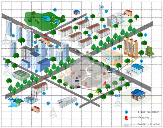
Figure 1. Sensitive area in WSNs.

2.2. Definition of Concepts

It is a primary and common way to estimate the position of the targets by the information of sensor nodes [26], and the energy consumption of communication mainly depends on the Euclidean distance between different nodes. K. Hadi et al. used the average distance between sensor nodes to estimate the target area [27]. The following context will introduce the key concepts and symbols appearing in the subsequent sections.

• Sensitive Areas (SA)

The monitoring area is a sensitive area (named SA), which is usually an irregular pattern, and the position of sensitive areas may shift or change throughout the WSNs within a certain time. Figure 1 shows that the marked range belonging to SA is called region of interest (named RoI), and sensor data are transmitted to the upper node through the backbone node in the WSNs [28]. The scenario of locating the SA involves acquiring the coordinates or grids of the sensitive areas in the WSNs through the preset threshold and the value of each sensor in the network.

• Sensor Sparse Matrix (SSM)

The sensor network provides a channel for data sinking from each single sensor node; however, the process and analysis of the data usually are arranged on the remote cloud or several high-performance clusters. Then, the above network can be abstracted into a digital matrix. Since most elements in the matrix are zero in the actual scenario, we call it a sparse matrix or sensor sparse matrix (SSM).

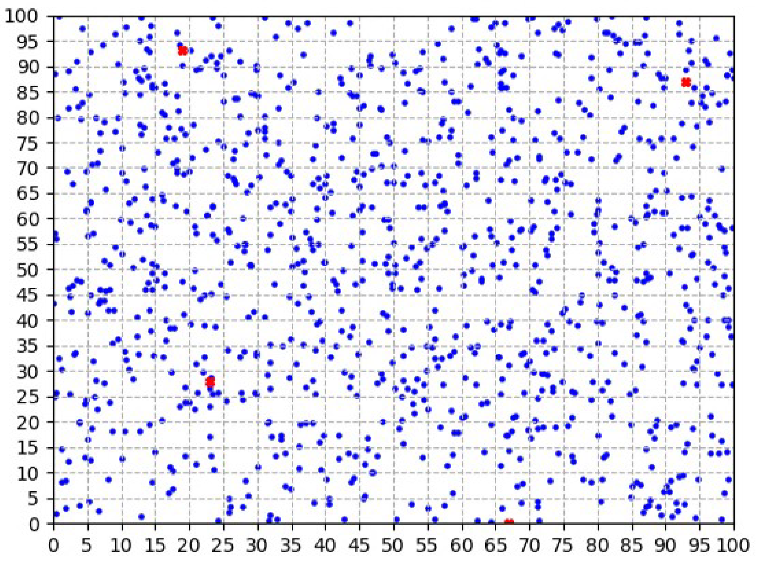
As shown in Figure 2, the entire WSN is divided into many grid cells, and every cell is associated with some sensors while building the WSN. Accordingly, we establish an $N\times N$ matrix model for clusters, and the value of each element of the matrix is the sum of all sensor data in one grid. There are many elements in the matrix that are 0 or below the threshold because of the data merger. The convolution-based continuous object localization algorithm (CCOL) proposed in this article works on this sparse matrix, and the convolution operation in CCOL rapidly achieves the position of target.

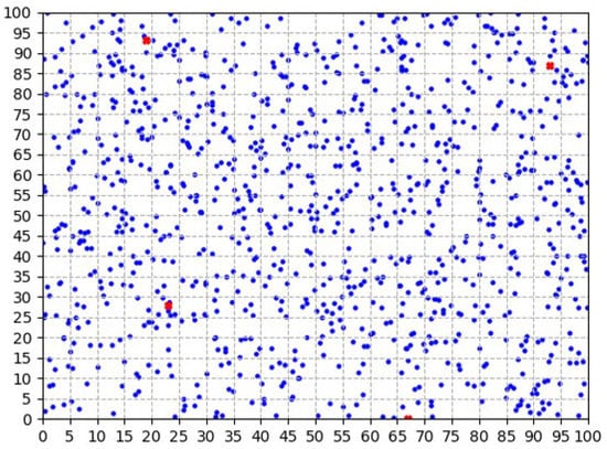
Figure 2. Distribution of sensor data.

• Convolution Kernel Matrix (CKM)

The matrix scope is related to the real size of WSNs. In other words, the larger the network scale is, the greater the number of grids, and the larger the corresponding matrix. Given the large size of the general grid matrix mentioned above in terms of the spatial distribution and mathematical operations, for example, in the sensor distribution in Figure 2, there is a $100\times 100$ SSM correspondingly. However, this type structure, or the size of the rows and columns of the two-dimensional matrix, could restrict the performance of the positioning algorithm to a certain extent. The convolution in the algorithm of CCOL slides the default kernel matrix through the original SSM ($N\times N$), and generates a new matrix that is smaller than the original. Therefore, the original matrix is partitioned into different blocks, and the sum of each block forms the result matrix. These serial operations complete the lossless fusion of sensor data and avoid the dispersion of continuous target data in the adjacent grids of WSNs.

In Equation (1), $\mathbf{A}$, the initial matrix of sensor data, is transformed to $\mathbf{B}$ through $\mathbf{C}$. This process is the convolution explained above. Meanwhile, it assumes that the default kernel matrix $\mathbf{C}$ is a $3\times 3$ matrix. After the convolution operation, the rows and columns of the result matrix $\mathbf{B}$ can be reduced to one-third of the original matrix. Therefore, the shrink ratio of $\mathbf{A}$ is related to the rank of the convolution kernel $\mathbf{C}$.

$$\begin{array}{ccc}\hfill {\mathbf{A}}_{m\times n}\times {\mathbf{C}}_{3\times 3}& =& {\mathbf{B}}_{k\times r},where\hfill \\ \\ \hfill {\mathbf{A}}_{m\times n}& =& \left(\begin{array}{cccc}{a}_{11}& a_{12}& \cdots & a_{1n}\\ a_{21}& a_{22}& \cdots & a_{2n}\\ ⋮& ⋮& \ddots & ⋮\\ a_{m1}& a_{m2}& \cdots & a_{mn}\end{array}\right)\hfill \\ \\ \hfill {\mathbf{C}}_{3\times 3}& =& \left(\begin{array}{ccc}{c}_{11}& c_{12}& c_{13}\\ c_{21}& c_{22}& c_{23}\\ c_{31}& c_{32}& c_{33}\end{array}\right)\hfill \\ \\ \hfill {\mathbf{B}}_{k\times r}& =& \left(\begin{array}{cccc}{b}_{11}& b_{12}& \cdots & b_{1r}\\ b_{21}& b_{22}& \cdots & b_{2r}\\ ⋮& ⋮& \ddots & ⋮\\ b_{k1}& b_{k2}& \cdots & b_{kr}\end{array}\right)\hfill \end{array}$$

(1)

From the matrix calculation in Formula (1), the data volume of the entire WSN decreases exponentially after the slide convolution. This decrease in turn reduces the workload of the computing nodes and saves energy in the sensor nodes.

• Mobile Nodes (MNs)

The mobile nodes(MNs) are mentioned when some emergency occurs in the target areas. The algorithm of MSSM addresses these problems. Once the target appears in some regions, it will inevitably cause anomalies in sensor data. The data are then aggregated and transmitted to the cloud servers or other clusters through the wireless network. After computing by the clusters, the mobile nodes respond to SA in accordance with the optimal energy consumption scheduling strategy. In the following experiments, we set different numbers of mobile nodes randomly in an $N\times N$ network (for example, the four red symbols of “X” shown in Figure 2), and customize and design a service scheduling strategy for WSNs.

2.3. Contribution and Solutions

In many references related to localization and tracking, the first step of most scenarios is planarization, and then, accurate positioning of the boundary follows. There are some popular planarization algorithms, including the Gabriel graph (G-G), relative neighborhood graph (RNG) and k-localized Delaunay graph (LDelk), etc. [29]. All of them can find the targets in WSNs but need to promote the accuracy of the object boundary. A large number of researchers, such as the authors of [10], have done a considerable amount of work based on these algorithms to improve the precise algorithm of the boundary area of continuous targets.

In this paper, our localization algorithm learns the algorithms [10,29] mentioned above in the storage and classification of sensor data; in particular, we employ the convolution matrix method to achieve the position perception of targets, and the proposed algorithm also has strong applicability in deployment schemes. The main research content and ideas of our work will be listed in the following context.

(1) Main research content

In the early stage, we surveyed the solution of continuous target localization and dispatching strategy of MNs in response to emergencies in WSNs. With the specific implementation of many algorithms proposed in different references, our research in this essay can be summarized as follows:

• Data fusion of continuous targets between grids

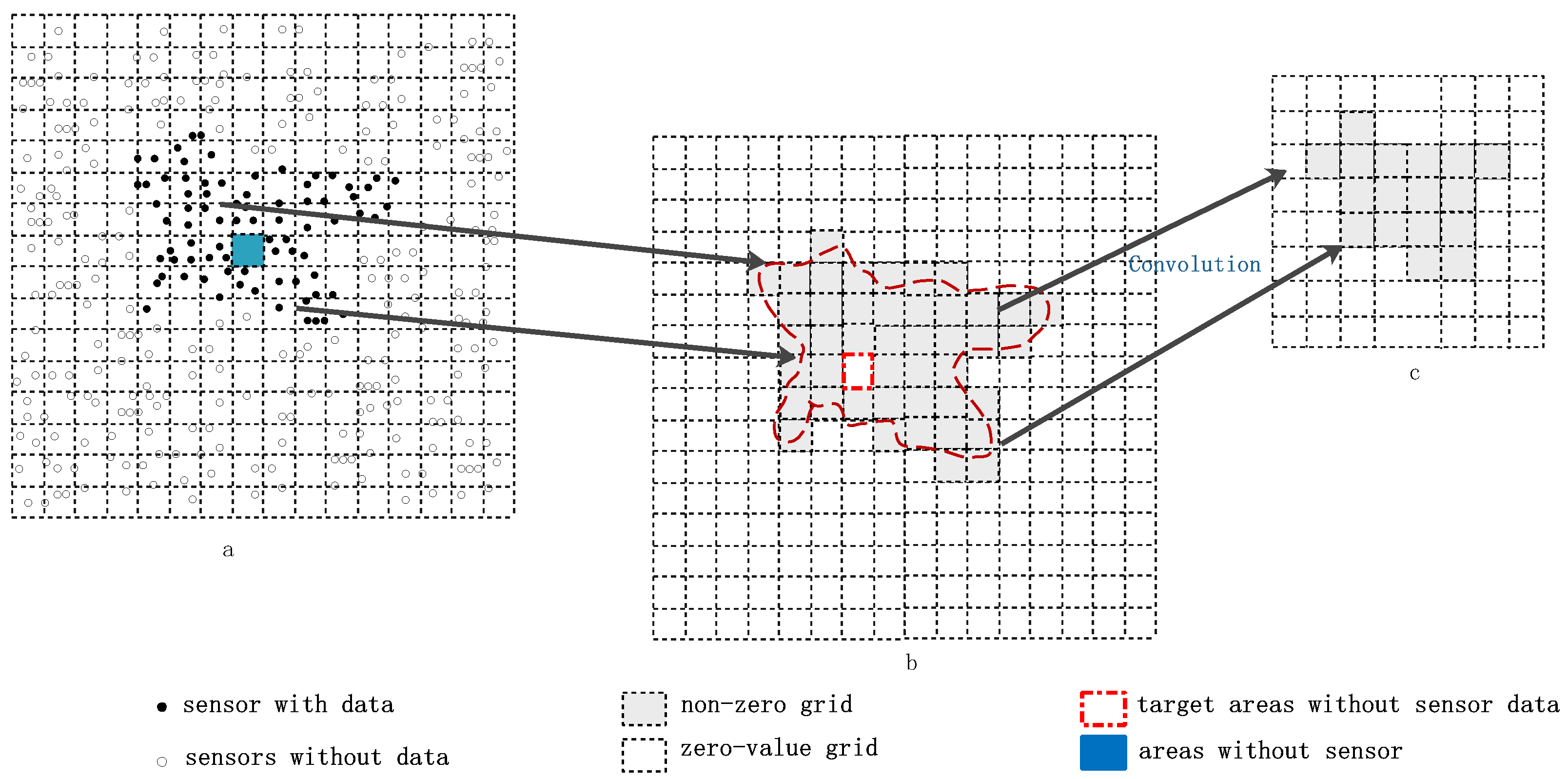
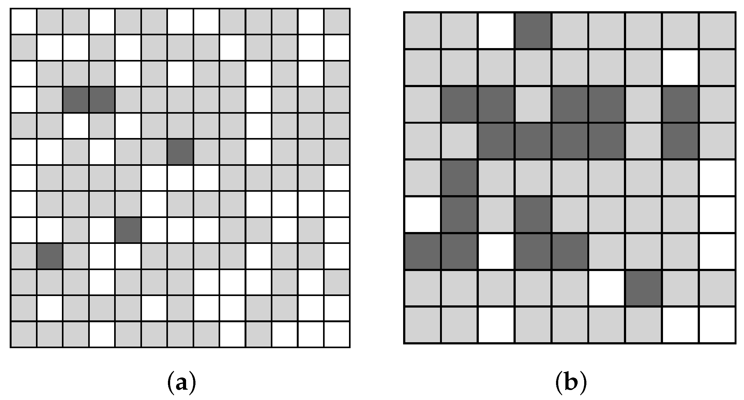
The value of grid data corresponding to the area where the target appears may be zero because of the random distribution or failure of sensors. Figure 3a shows that the irregular area covered by the black points is an SA, and there is a blue grid without any sensor in this region (in fact, this area should also be the subject of our supervision). Figure 3b shows a rough scope of the target combined by gray grids, and the red dotted line marks the boundary of the target; however, there is a blank grid mapping to the blue grid in Figure 3a. Assuming the size of CKM is $2\times 2$, through the convolution operation, the grid matrix ($8\times 8$) in Figure 3b becomes the result matrix of Figure 3c whose size is $4\times 4$. Interestingly, the special blank grid in Figure 3b disappears in Figure 3c.

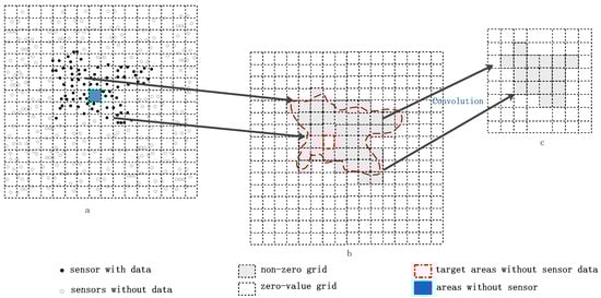
Figure 3. Fusion process of sensor data. (a) is the original network and the distribution of the sensors data; (b) is the marked SA including a special grid without sensor; (c) is the fusion result of the sensors data.

• Matrix deflation

The value of each sensor node is transmitted by the sink nodes, and the cluster maps the data to the grids used in the localization algorithm according to the coordinate relationship. After the gridding, every sensor node belongs to one cell and is stored in a two-dimensional matrix. Along with the expansion of WSNs, the data may grow exponentially, which requires a vast computing resources of the clusters. However, we notice that most elements of the matrix in WSNs are zero, which is why we call this matrix a sparse matrix. Specifically, it is for this reason that we provide a good idea to reduce the order of the matrix.

The sliding convolution proposed in this essay is employed to solve the excessive calculations. It divides the matrix into several sub-matrices of the same size as the convolution kernel matrix, sums the sub-matrices, maps the result to a new matrix (matrix B in Formula (1)), and completes the deflation of the initial matrix. This matrix is also an important part of the simulated experiments.

• Strategy of multi-node and service scheduling

The scheduling of emergency node(s) is another crucial problem that we study [24]. We focus on how to improve the response rate of emergencies of WSNs in this article and try to establish a scheduling mechanism that makes the resource consumption of the whole network as small as possible. Many researchers are concerned about this issue; for example, an approach of path planning for mobile nodes was proposed in [27] that could efficiently solve network congestion.

The area of continuous objects in the network is divided into several adjacent grid matrices under the sliding influence of the convolution kernel. Moreover, the strategy of the mobile scheduling is a simulation of the emergency response process. This simulation could improve the overall reaction speed of the WSNs and the allocation efficiency of the resource when some events occur. In addition, this approach has a great significance in practice, such as in the manual intervention evacuation of human traffic or the spread of dangerous targets.

(2) CCOL Model

The algorithm of CCOL works on the grid data of WSNs, and the detailed process has been discussed in the above sections. Given the discreteness and sparseness of data in the sensor grids, rapid matrix degradation is attractive when the volume of data in WSNs is massive. Therefore, it is natural that detection and tracking for continuous objects will be completed by this operation. However, if the continuous target area is very large, the number of grids is more than the size of the convolution kernel matrix, and the whole SA may be decomposed into multiple feature grids.

The research in this article has been divided into the following two steps: target localization and multiple node scheduling. The former mainly accomplishes the reduction of a matrix for sensor data grids and builds the relationship between the convolutional characteristic region and the real areas in WSNs. The latter step verifies the strategy of multi-MNs in WSNs, and the simulation experiment has been designed to justify the rationality.

Additionally, we assume that the energy consumption in the MN scheduling abides by the following Equation (2) in the experiments.

$$E=\frac{D_{coll}\left(s_i\right)}{d_{coll}}+\frac{D_{com}(s_i,s_j)}{d_{com}}+\frac{D_{exe}\left(s_i\right)}{d_{exe}}$$

(2)

In Equation (2), $d_{coll},d_{com},d_{exe}$ are constants; $d_{coll}$ represents the total data that can be collected by consuming a unit of energy; $d_{com}$ represents the total data transferred from $s_i$ to $s_j$ by consuming a unit of energy; $d_{exe}$ represents the total data computed at $s_i$ by using a a unit of energy. Meanwhile, $D_{coll}\left(s_i\right)$ is the amount of data collected at $s_i$; $D_{com}(s_i,s_j)$ is the amount of data transferred from $s_i$ to $s_j$; $D_{exe}\left(s_i\right)$ is the amount of data executed at $s_i$.

The algorithms proposed in this paper will efficiently save the energy consumed in computations for the whole network. In this model, the main energy cost in WSNs is spent on the data collection and transmission, and this MN scheduling approach will expand the lifetime of WSNs. Therefore, the optimization of the MN’s emergency dispatching scheme mainly refers to the geographic distance to the sensitive area and real-time working status of the MN. Subsequently, the strategy will plan the motion trajectory for the MNs in WSNs.

3. Problem Formulation and System Model

In this section, we mainly discuss the data processing model of the CCOL algorithm. In the initial state, each sensor node reports its position to the clusters deployed in the cloud. Then, each sensor node enters the dormant state until an emergency occurs at a certain time point, at which the node is woken up and uploads the sensor data to the sink nodes periodically or when they sense some abnormalities. According to different models, the algorithm running on the computing centers will fulfill the target localization and scheduling.

3.1. Settings for the Convolution Kernel

The settings of the convolution kernel are one of the important issues in our research. A large discrepancy in the calculation results of the original data matrix will occur when the algorithm employs different convolution kernels. The results of the operation of the original data matrix by different convolution kernels will be very different. In this essay, we take a matrix that is a $K\times K$ unit square ($K=3$ in the experiment), and the scale of the original matrix is reduced by $1/K$. However, the process of setting the value of K depends on the specific size of the WSNs. Generally, the parameter K and the coverage of WSNs are proportional. Consequently, the value of K should increase or decrease as the size of WSNs changes.

The convolution matrix can effectively compensate for the lack of data in continuous target areas. For example, a continuous target may dominate multiple grids; once the sensor in this area fails or the distribution is missing, it is not appropriate to localize the boundary solely according to real sensor data from WSNs. Convolution might merge the neighbor grids, which have no data but cover the target areas, into one element in the convolution matrix. Due to following the formula (Equation (4)), the operation will non-destructively retain the original features of the continuous targets during the whole convolution process.

3.2. Sensor Data Processing Model

The sensor data processing model converts the data collected by the sensors into a matrix for target positioning, and it can be roughly divided into the two stages listed in the following context.

(1) Mapping to the grids

Sensors are randomly distributed throughout the network in WSNs, and each sensor can correspondingly gain a value. These values are assigned to different grids in accordance with their position. Briefly, one grid is taken as the minimum unit for data processing in this paper, and the value of the grid is the cumulative sum of all sensor data in it (Equation (3)).

$$a_{ij}=\sum _{i\le x\le i+1,j\le y\le j+1}{S}_{xy}$$

(3)

In Equation (3), $i,j$ is the index of the row and column of the grids, respectively; $S_{xy}$ is single value of the grid ($x,y$), in which the x and y are limited by $i\le x\le i+1$ and $j\le y\le j+1$, respectively. Each $a_{ij}$ is the cumulative sum of grid ($x,y$).

(2) Sliding convolution

According to the computing method involved in Equation (3), the entire network is replaced by the following matrix in Equation (4). Each element ($a_{ij}$) in the matrix is obtained by superposing several $S_{xy}$. The sliding convolution operation serves to ensure that the CKM multiplies a matrix that has the same size as CKM and is combined by $a_{ij}$. The whole calculation process is divided into two parts:

Step 1: Pre-arrangement of the matrix

Once the WSN is blocked by the default size, the number of rows or columns of the aforementioned matrix can be ensured.

$$\left(\begin{array}{cccc}{a}_{11}& a_{12}& \cdots & a_{1\left(nK\right)}\\ a_{21}& a_{22}& \cdots & a_{2\left(nK\right)}\\ ⋮& ⋮& \ddots & ⋮\\ a_{\left(mK\right)1}& a_{\left(mK\right)2}& \cdots & a_{\left(mK\right)\left(nK\right)}\end{array}\right)$$

(4)

In this paper, if the number of rows and columns of the original sensor data matrix is not an integer multiple of the number of rows and columns of the CKM, it will insert certain zero rows or columns into the source matrix to facilitate subsequent operations.

For example, a $100\times 100$ network is blocked by a $5\times 5$ grid, which will yield a $20\times 20$ matrix. If the size of CKM is $3\times 3$, we should add one zero-row and one zero-column to obtain a $7\times 7$ convolution result matrix. As shown in the formula, if the CKM is a $K\times K$ square matrix, the size of the original matrix will be prepared as $mK\times nK$.

Step 2: Convolution

During the processing of convolution, the original matrix in Equation (4) has been distributed to $m\times n$ blocks following the rule illustrated in Equation (5). Therefore, each block ${\mathbb{A}}_{ij}$ is a $K\times K$ square matrix marked by $\mathbf{A}$, and the matrix (Equation (4)) shrinks to $\mathbf{A}$ (Equation (6)).

$${\mathbb{A}}_{ij}=\left(\begin{array}{ccc}{a}_{(i\times K)(j\times K)}& \cdots & a_{(i\times K)\left(\right(j+1)\times K-1)}\\ a_{(i\times K+1)(j\times K)}& \cdots & a_{(i\times K+1)\left(\right(j+1)\times K-1)}\\ ⋮& \ddots & ⋮\\ a_{\left(\right(i+1)\times K-1)(j\times K)}& \cdots & a_{\left(\right(i+1)\times K-1)\left(\right(j+1)\times K-1)}\end{array}\right)$$

(5)

$$\mathbf{A}=\left(\begin{array}{cccc}{\mathbb{A}}_{11}& {\mathbb{A}}_{12}& \cdots & {\mathbb{A}}_{1n}\\ {\mathbb{A}}_{21}& {\mathbb{A}}_{22}& \cdots & {\mathbb{A}}_{2n}\\ ⋮& ⋮& \ddots & ⋮\\ {\mathbb{A}}_{m1}& {\mathbb{A}}_{m2}& \cdots & {\mathbb{A}}_{mn}\end{array}\right)$$

(6)

We symbolize the CKM as matrix $\mathbf{C}$ (Equation (7)), a unit square of $K\times K$, of which all elements are 1.

$$C={\left(\begin{array}{ccc}1& \cdots & 1\\ ⋮& \ddots & ⋮\\ 1& \cdots & 1\end{array}\right)}_{K\times K}$$

(7)

Equation (8) gives the calculation method of $r_{ij}$, which is a numerical value that corresponds to the result of each ${\mathbb{A}}_{ij}$ (Equation (6)) multiplied by $\mathbf{C}$ (Equation (7)).

$$r_{ij}=\sum _{\begin{array}{c}i\times K\le w\le (i+1)\times K-1\\ j\times K\le y\le (j+1)\times K-1\end{array}}{a}_{wl}\times c_{wl}$$

(8)

Compared to the original matrix (Equation (4)), the result matrix $\mathbf{R}$ (Equation (9)) has the same size of $\mathbf{A}$ (Equation (6)). In other words, it has been shrunk by K. Therefore, this approach can solve the problem of matrix deflation.

$$\mathbf{R}=\left(\begin{array}{cccc}{r}_{11}& r_{12}& \cdots & r_{1n}\\ r_{21}& r_{22}& \cdots & r_{2n}\\ ⋮& ⋮& \ddots & ⋮\\ r_{m1}& r_{m2}& \cdots & r_{mn}\end{array}\right)$$

(9)

$\mathbf{R}$ in Equation (9) is the result matrix, and each element ${\mathbf{r}}_{ij}$ in matrix $\mathbf{R}$ can represent an area of ${(K\times gsize)}^2$ in WSNs, where K is the number of rows of the CKM, and $gsize$ is the side length of each mesh in WSNs. Then, the value of $R_{wl}$ can be considered as the eigenvalue of the corresponding region. Thus, when a continuous target arises in the surveillance area, a certain $R_{wl}$ corresponding to the target will differ with respect to the neighboring areas. Therefore, this is the primary reason that object detection can be accomplished by using this model.

3.3. Multimobile Service Node Scheduling Model (MSSM)

The MSSM refers to the treatment method in [30] and adopts a dynamic and greedy idea. Its purpose is to keep each MN as busy as possible at the same time and to reduce the waiting time for emergency events in sensitive areas. This section will describe this model in detail.

At the beginning, we make the following assumptions: $Set\left(M_i\right)$ is the set of MNs, $Set\left(O_i\right)$ is the set of grids of SA, and the $Set(M_k,O_l)$ is the set of distances from any MN to the target areas.

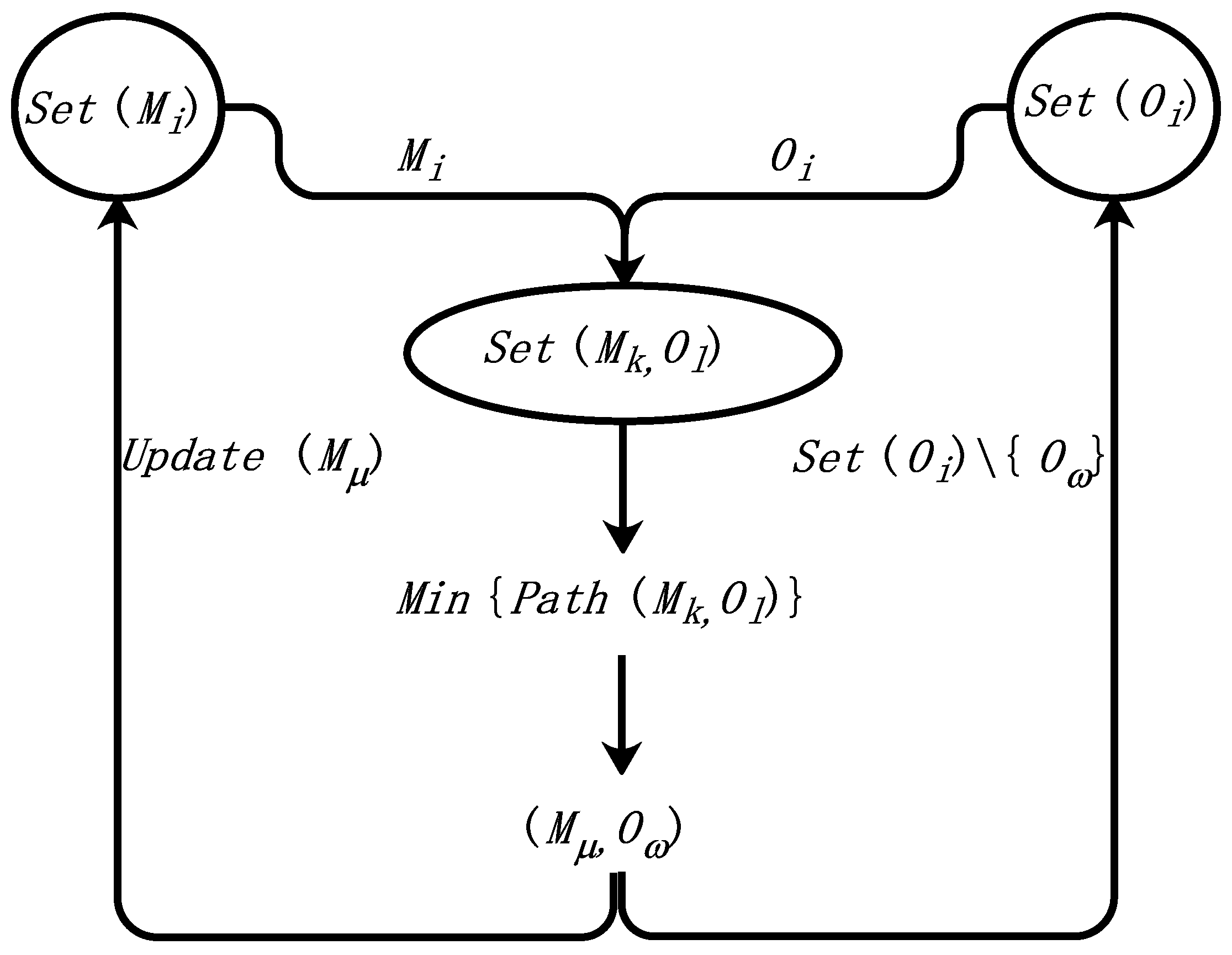
This model (shown in Figure 4) mainly involves the operations among $Set\left(M_i\right)$, $Set\left(O_i\right)$ and $Set(M_k,O_l)$. According to the minimum element of $Set(M_k,O_l)$, it iterates and updates the $Set\left(M_i\right)$, and removes the element $O_{\omega }$ from $Set\left(O_i\right)$. This process is repeated until the $Set\left(O_i\right)=\mathrm{\varnothing }$ and is then terminated.

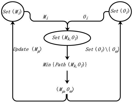
Figure 4. Multimobile service node scheduling model.

The greedy algorithm will find a suitable mobile service node and one shortest scheduling path to respond the SA, and it can also decrease the number of leisure service nodes and minimize the energy consumption throughout the scheduling process.

4. Core Algorithm

The two algorithms of CCOL and MSSM discussed in this paper address the target detection and emergency scheduling in WSNs. The following context will explain the principle and process of each algorithm.

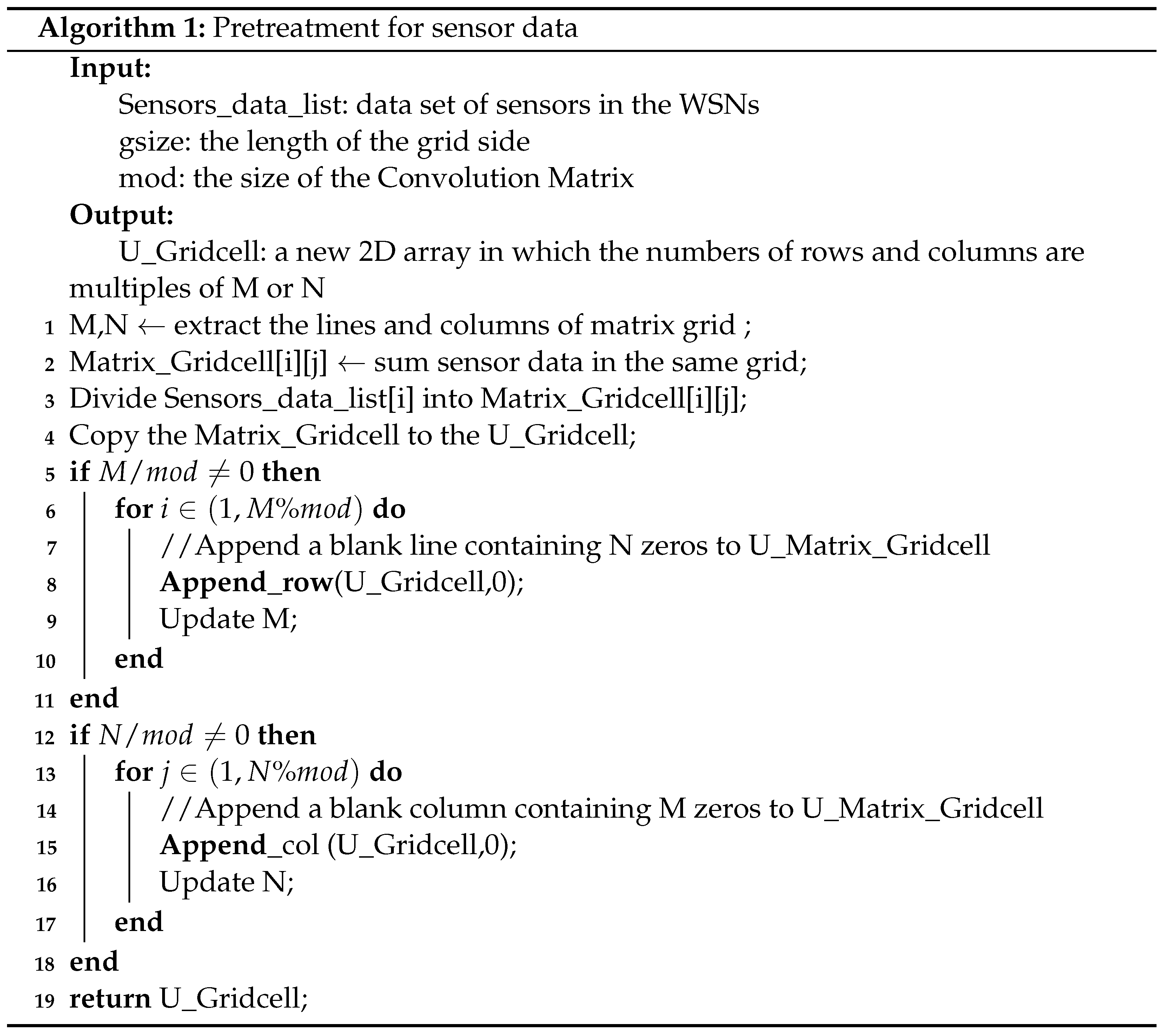
4.1. Pretreatment of Sensor Data

The pretreatment of sensor data in WSNs contains two tasks: blocking the WSNs and rounding the numbers of the row or column of the matrix. After the preprocessing step, we gain a new blocked grid matrix. The formula of this step refers to the model in Section 3.

After padding and aligning, Algorithm 1 returns a new matrix (U_Matrix_Gridcell), whose rows and columns can be divided by the number of rows and columns of the convolution matrix. In addition, the sensor’s data are mapped to the grids.

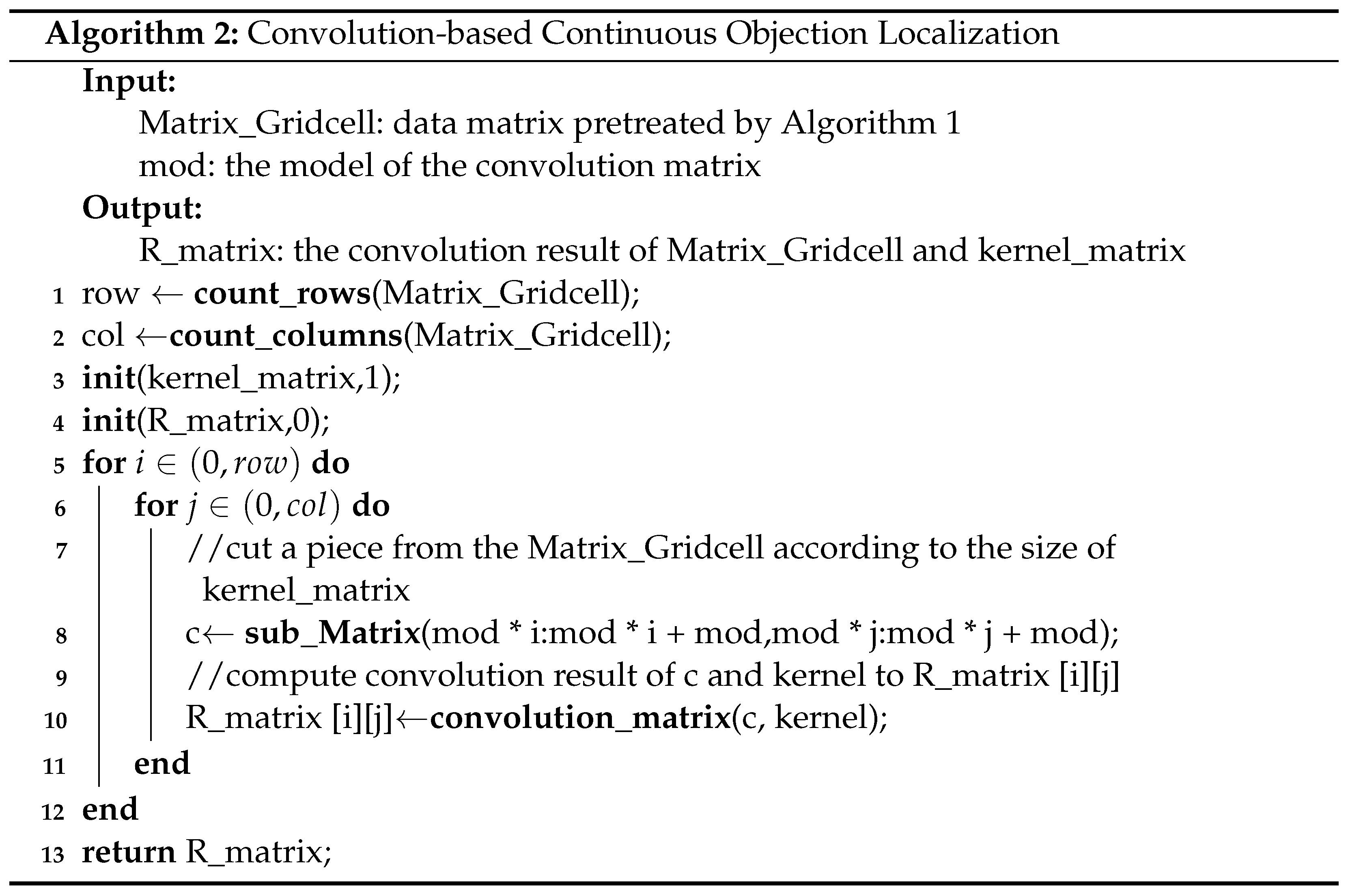
4.2. Convolution-Based Continuous Object Localization Algorithm (CCOL)

After the process of Algorithm 1, the sensor data are stored in Matrix_Gridcell. According to the index (i,j) in the array of R_matrix, it converts the coordinates of the first element ($mod\times i,mod\times j$) and the last element ($mod\times i+mod,mod\times j+mod$) of the matrix subblock involved in each convolution and then obtains the subblocks c that will take part in the convolution with $kernel\_matrix$. At the end, the result will be stored in $R\_matrix\left[i\right]\left[j\right]$, and Algorithm 2 will return the entire array of $R\_matrix$.

In fact, the nonzero elements in the R_matrix should be focused on. Each nonzero element relates to an SA in WSNs, and the SAs in WSNs are marked in the R_matrix by the grid index. Therefore, the reverse process is the localization for continuous targets. For instance, one nonzero value may be mapped to an emergency (a gas disaster, the dense flow of a crowd or an abnormal environmental event and so on), and the system scheduling will take some emergency measures to react to the SA in the special scenario.

4.3. Multimobile Service Node Scheduling Algorithm (MSNS)

Following the convolution of Algorithm 2, we set an alert threshold such that $S_{xy}$ is either 0 or 1 (shown in Equation (10)).

$$S_{xy}=\left\{\begin{array}{ccc}\hfill 0& & ifthetargetexists\hfill \\ \hfill 1& & ifthetargetdoesnotexist\hfill \end{array}\right.$$

(10)

The data of the matrix $\mathbf{A}$ are accumulated by Equation (8), and the cumulative result reflects the degree of the SA emergency. Once the present threshold is reached, it will start the process of scheduling and reply to the SAs. Moreover, convolution can overcome the shortage of discreteness of sensor data in the localization such that one continuous target maybe divided into several neighboring elements in the result matrix. Therefore, this condition provides a solution for MN scheduling. Accordingly, the dynamic scheduling algorithm is divided into two situations for different sizes of SAs:

(1) Limited in one grid

If the target is a single object (such as a car or fire point), Algorithm 3 is a special case of the multimobile service node scheduling algorithm. The sensitive area corresponding to the target is so small that there is only one grid corresponding to it. In this case, the scheme is relatively simple: we simply select a node that is closest to the SA with the most energy to provide services. The detailed algorithm is described in the following (Algorithm 3).

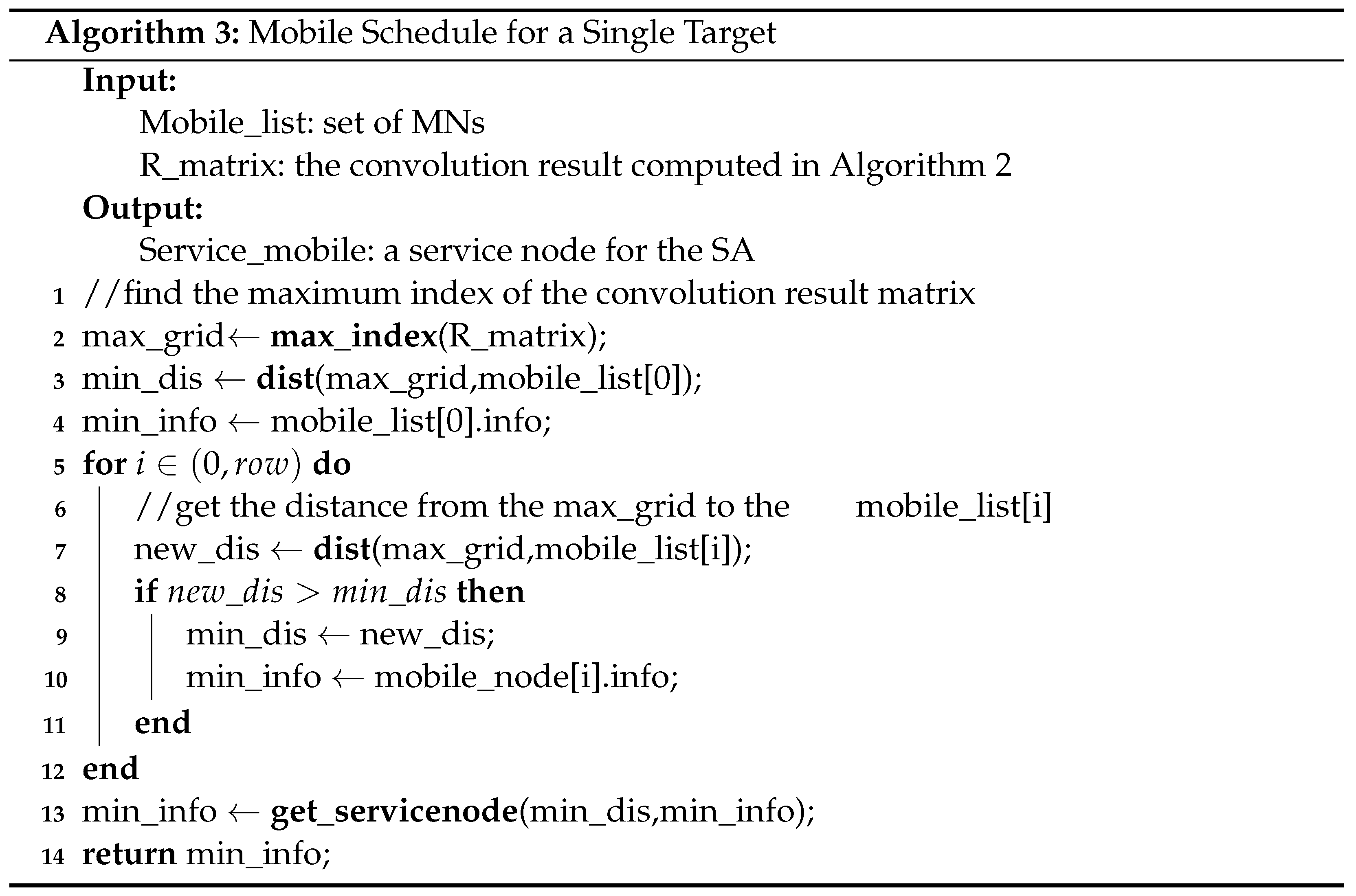
Once the SA is served by the MN, this service node will move to the area marked by min_info that corresponds to the emergency. Moreover, it updates the remnant of energy and the current position.

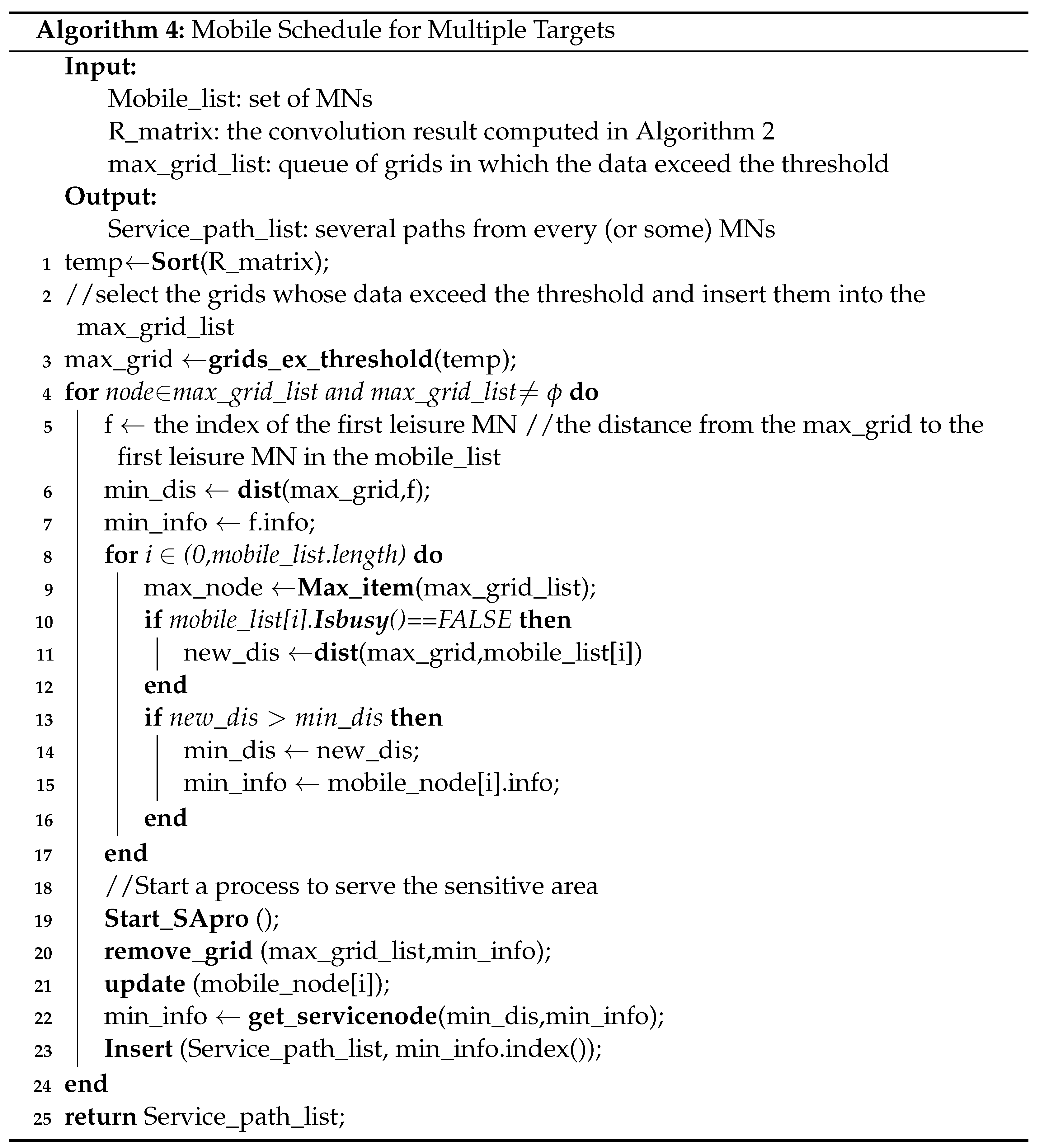
(2) Covering many grids

Algorithm 4 is a general case of multimobile service node scheduling. The SA always exists throughout several grids and has an irregular shape.

Convolution will map the target to some adjacent grids whose values exceed the threshold, which will greatly narrow the search range of the target area. This effect could increase the efficiency of the emergency response capability in coupling with the MSNS algorithm. The details of Algorithm 4 are as follows.

The difference between Algorithms 3 and 4 is that line 19 (Algorithm 4) takes some threads to serve the SAs, and the rest of them are almost the same.

5. Experimental Simulation and Analysis

Based on the aforementioned discussion, simulation and verification of the experiment are proposed in this section. We compare the performance of CCOL to the G-G and RNG, analyze the consumption of different strategies, and prove the feasibility of the algorithm proposed in the article.

5.1. Simulation Experiment

The experiment simulates a $500\times 500$ wireless sensor network that randomly deploys 300 sensors. The $500\times 500$ network represent a region related to the size of the grid, we do regard it as a residential area or an urban area. Without loss of generality, 300 sensors are assigned to different grids randomly. In the program, there is a variable length list of MNs, in which the position and the remaining energy of the node are stored. The size of the grid is $20\times 20$, so the whole network is divided into $25\times 25$ grids, and a square matrix of which all elements are 1 is appointed as the CKM. The detailed experimental process is as follows:

Step 1: Sensor maps to the grid

The position of the sensors is random. To facilitate the sliding convolution, sensor data need to be preprocessed at the beginning. According to Algorithm 1, the network ($25\times 25$) is expanded with different kernel matrices. In our experiment, we takes two CKMs ($2\times 2$ or $3\times 3$) to deal with data grid corresponding to the original network.

Step 2: Convolution with the CKM

The processed data in the matrix are convolved with the $3\times 3$ operator and generate a result matrix that is only one-third of the original grid matrix.

Step 3: Localization of the SA

If there are some values that exceed the threshold, the program will revert to the original position from the location of exceeded values.

Step 4: Scheduling MNs

In the above steps, the SAs in WSNs are detected. A dynamic and greedy scheme is implemented, and several MNs in the list should be selected to respond to the different SAs (Algorithms 3 and 4).

5.2. Results of the Experiment

(1) Data of the matrix

The cumulative sum determines the data in each grid, each sensor will be set to a random value (0 or 1), and then, we accumulate the results in one grid unit that has the important reference data in the target localization.

Figure 5 presents a visual representation of the matrix ($25\times 25$), and grid areas without sensors are indicated by black, while the gray denotes the areas with sensors. Then, the program can judge whether the value of the grid exceeds the threshold.

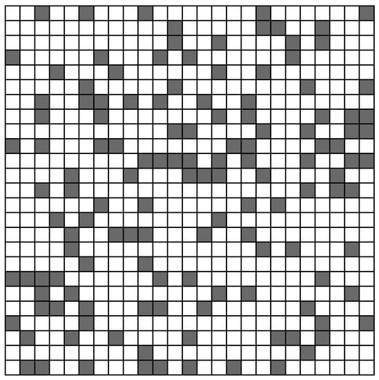
Figure 5. Original data grid.

According to the steps in Section 5.1, different CKMs need different sizes of Prepossessed data grid. As shown in Figure 6a is the pre-processing matrix required by the $2\times 2$ CKM, and Figure 6b is the pre-processing matrix required by the $3\times 3$ CKM.

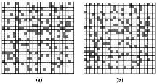
Figure 6. Data of grid. (a,b) is different pre-processing results with different CKMs, there is one more blank row and column a than that of b. (a) Pre-processing data grid with $2\times 2$ kernel. (b) Pre-processing data grid with $3\times 3$ kernel.

(2) Localization of SAs

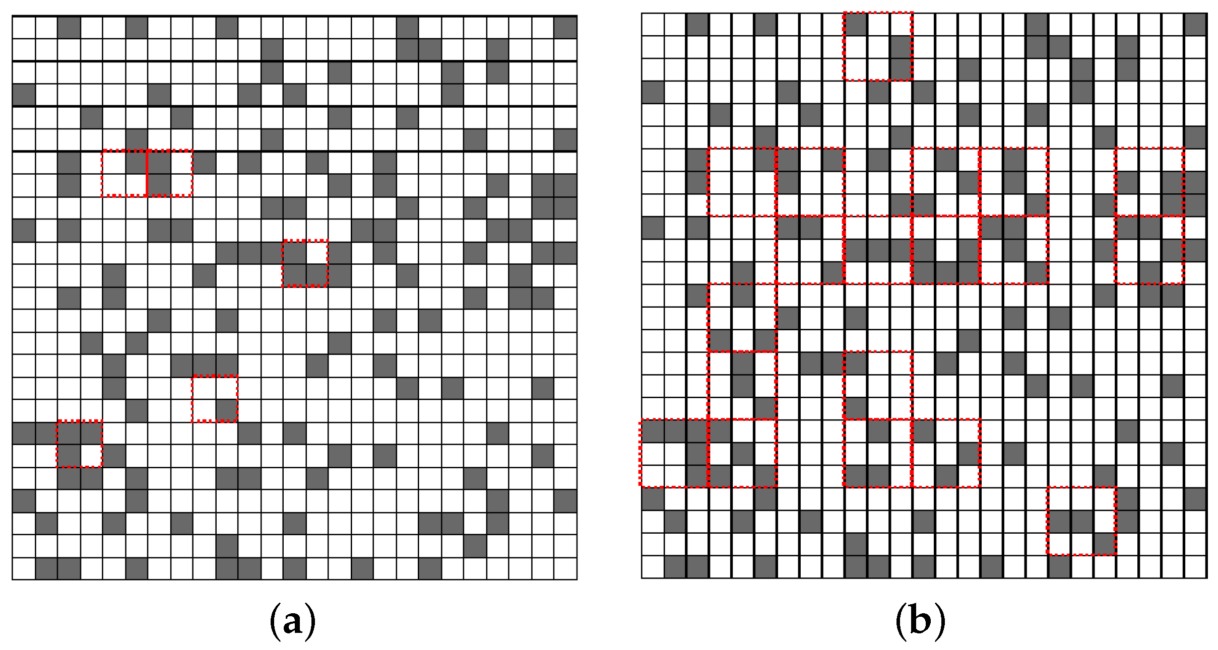
In the experiment, we assume the warning threshold is 3. The grids whose value reaches the threshold are indicated in these matrix. As shown in Figure 7, when we take $2\times 2$ and $3\times 3$ CKM, the position, number and the areas of targets in the grid are various.

Figure 7. Convolution result matrix. Because of the various sizes of CKM, the number of row and column of result matrices is different. (a) Convolution result Matrix with $2\times 2$ kernel. (b) Convolution result Matrix with $3\times 3$ kernel.

In Figure 7a,b, the darker areas are the SAs whose value exceeds the threshold, and they are the areas that we should closely monitor. The lighter areas and the blank areas are the SAs whose value does not reach the threshold, and we should not pay attention to these areas. Obviously, the darker areas in Figure 7a,b respond the range of the SAs are not equal. Therefore, the smaller the convolution kernel, the more accurate the positioning accuracy should be in theory. When the size of CKM is increases, the its corresponding area also becomes larger, and the positioning accuracy decreases.

According to the CCOL algorithm, we can get darker areas shown in Figure 8. Each darker region corresponds to a certain area in Figure 7, this process is the inverse of CCOL. So we can mark the darker areas by red dotted lines in Figure 8.

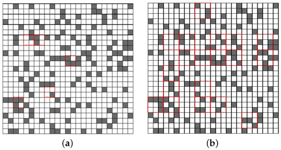
Figure 8. Marked SAs. (a) Marked SAs with $2\times 2$ kernel. (b) Marked SAs with $3\times 3$ kernel.

In Figure 8, the continuous targets can be distinguished by the darker grids, since they usually are localized by a series of irregular contiguous darker grids because of differences in shapes or sizes. Figure 8a,b are the location of SAs marked by different CKMs in the original network.

(3) Selecting Service nodes and Scheduling Paths

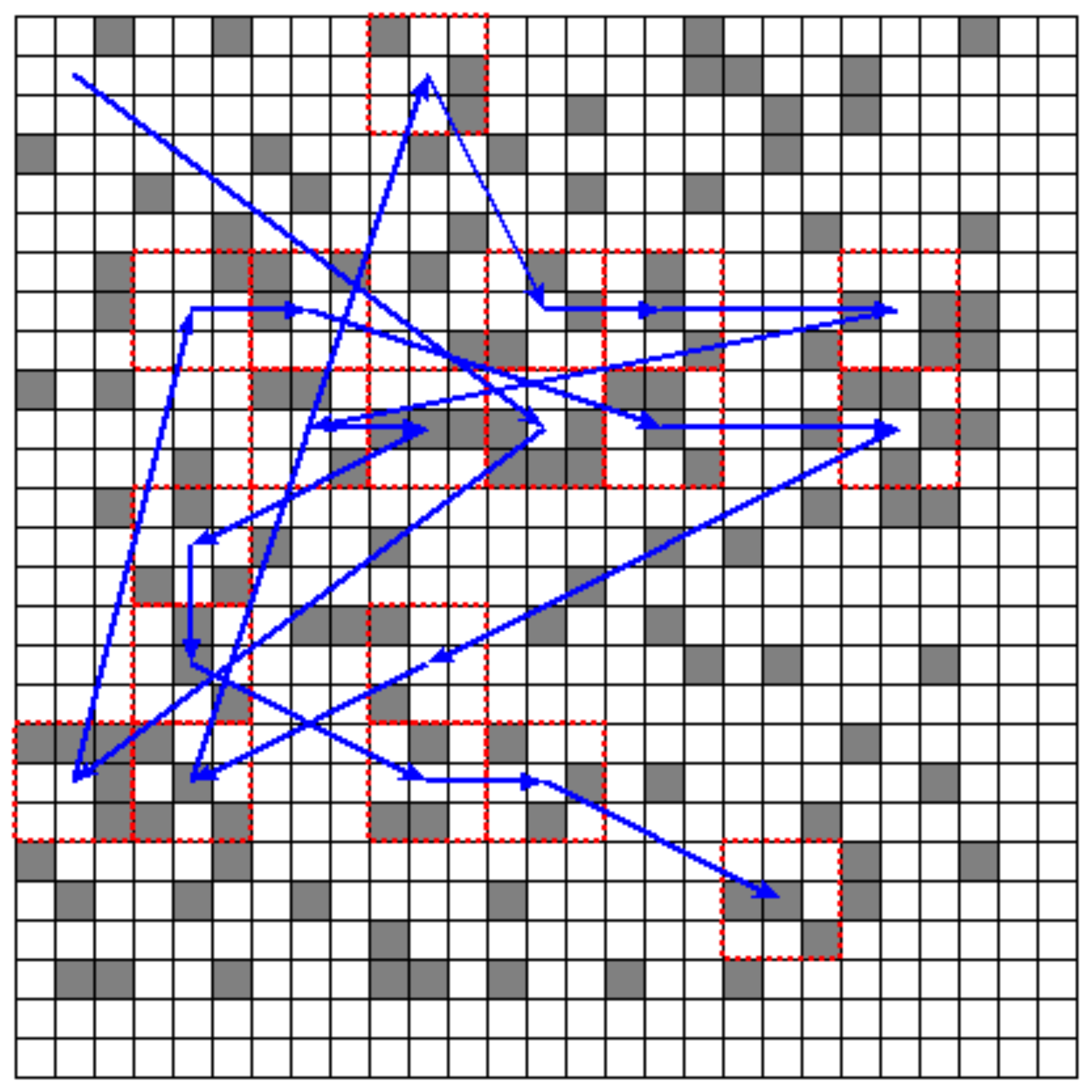
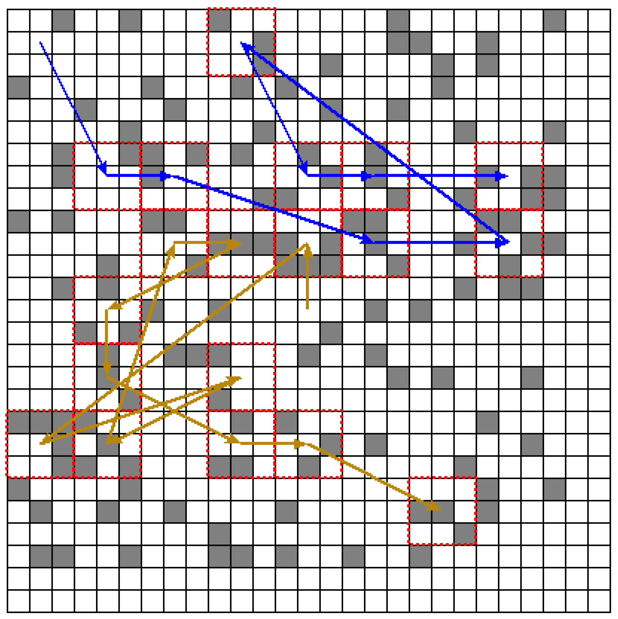
As a result of the aforementioned steps, they have proved that the size of CKM could impact the accuracy of target location in WSNs. However, the improvement of accuracy will inevitably increase the calculation of convolution operation. Therefore, a optimal CKM is very necessary. In order to verify the method mentioned above, we design a multi-node service scheduling. The scheduling with various numbers (1, 2, 4, and 8) of MNs serves the SAs in Figure 8, so we can plan the paths of MNs and record the energy consumption under different policies. We take Figure 8b as an example, and find 19 SAs that need to be served in total. The following is the path selection of different numbers of MNs.

• Path for a single node

The position of the single node was randomly set at $(2.3,5.01)$, according to the strategy and distribution of WSN, and its mobile path is drawn in Figure 9 by blue arrows.

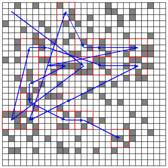
Figure 9. Path of a single node.

• Path for double nodes

If there are two service nodes, their position is set at $(2.3,5.01)$ and $(250,258.85)$. Since the same scheme is used, 19 SAs in Figure 8b were responded to. One of the nodes deals with 8 SAs, and the other node served 11 SAs. Their paths are drawn by different lines in Figure 10.

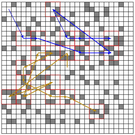
Figure 10. Path of a double node.

When the number of nodes increases to 4 or 8, the experimental results are similar to the above two cases, so we do not describe them redundantly.

5.3. Comparison and Analysis

In this section, the CCOLis compared with G-G and RNG algorithms, the depletion of each stratagem is counted, and the advantage and feasibility of the solution proposed in this essay are analyzed.

(1) Time Complexity

G-G and RNG are classical algorithms among the target localization approaches in WSNs, and a rough boundary can be found by them, similar to the CCOL. However, the CCOL is better than others in terms of the cost of time or execution. In Table 1, we find the merits of CCOL.

Table 1. Performance comparison.

Algorithm	Time Complexity	Recursion
G-G	$O\left(nlogn\right)$	Yes
RNG	$O\left(n^3\right)$	No
CCOL	$O\left(n^2\right)$	No

(i) G-G is lower than CCOL in terms of time complexity. However, the cost of the G-G is much more than the others because of the recursive call.

(ii) However, while RNG executes in the same manner as CCOL, the time complexity of $O\left(n^3\right)$ is higher than that of G-G and CCOL.

What needs to be emphasized is that G-G and RNG are based on geometry theory; however, the CCOL is generally based on grids. There may be some differences between them. If we want to obtain more accurate SAs, a precise algorithm must be employed to address the results of these algorithms.

Despite the advantages of CCOL compared with G-G and RNG, CCOL’s time complexity is still $O\left(n^2\right)$ which can be further optimized, while CCOL is usually deployed on high-performance devices such as remote servers or edge servers, considering the low-coupling correlation of grid data in the convolution process, parallelized program may be a better optimization solution whose time complexity is not changed nevertheless.

(2) Energy consumption of the WSN

In comparison to other algorithms, the CCOL proposed in this article might prolong the lifetime of the network. All of the WSNs will lose the same energy to complete the collection, transmission and so on. In the same network topology, other algorithms increasingly need more nodes to participate, but the CCOL does not. Most jobs of CCOL are finished on the center nodes or cloud servers; therefore, it is not necessary for any nodes to cooperate. Consequently, this approach could improve the utilization of the sensors in WSNs.

(3) Energy Comparison of MNs

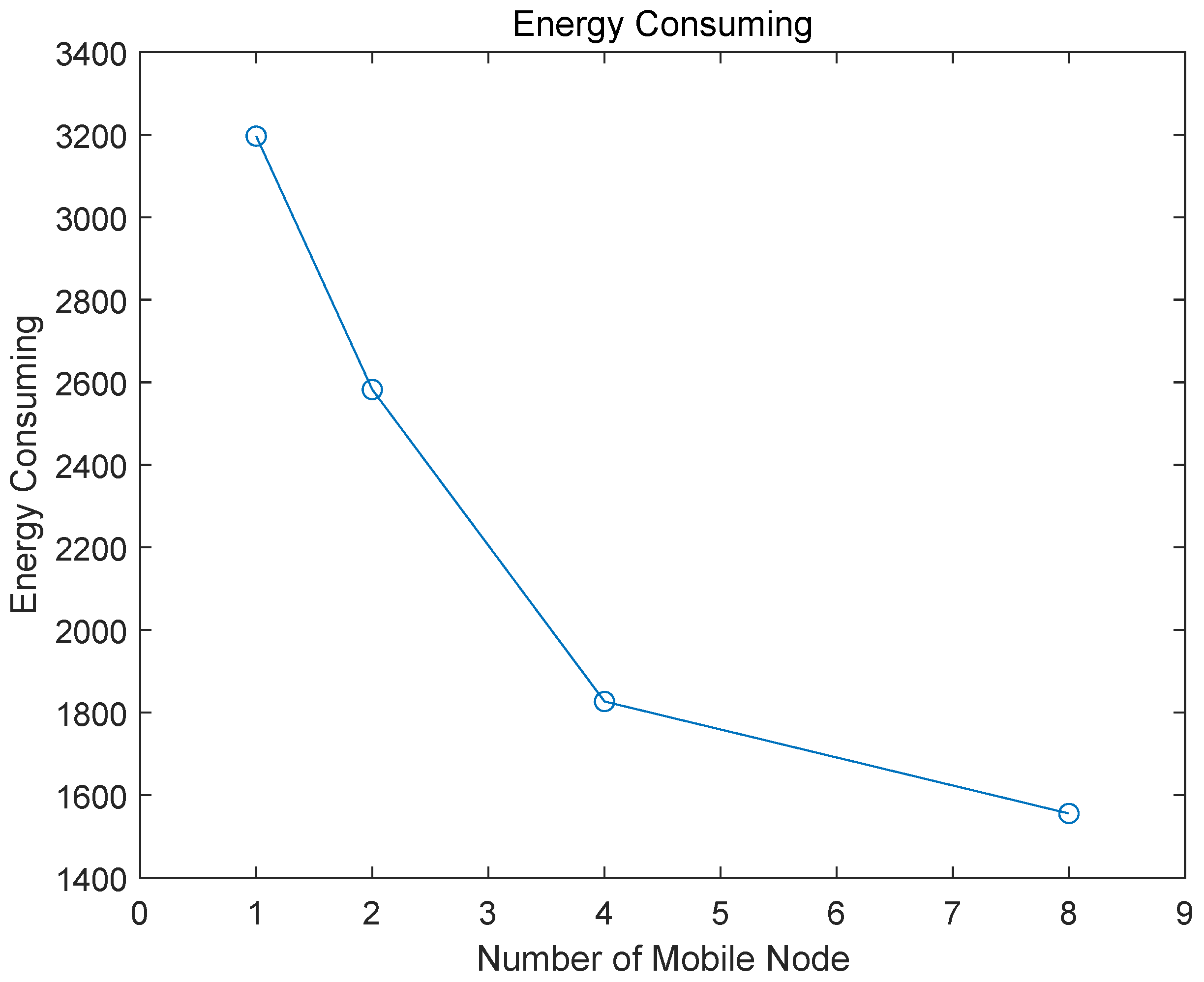
In the experiment in this essay, each node is set at 4000 points as the initial energy, and the energy consumption is calculated according to the distance $(E\left(d\right)=dis(p_1,p_2))$ from the service node to the SA. Figure 11 is the energy change of different numbers of nodes. Judging from the changing trend, as the number of mobile nodes increases, their total energy consumption tends to decrease dramatically.

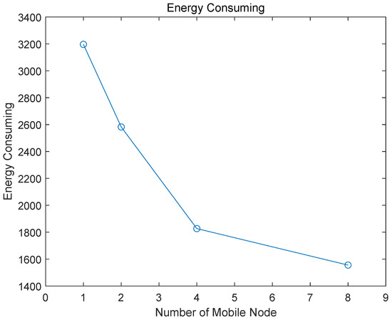
Figure 11. Trend of energy consumption.

(i) The change is obvious from 1 to 4, but this trend becomes gentle with the increase in the number of nodes.

(ii) When the number of MNs reaches 8, there are two service nodes that are not working, which is a waste of resources.

Given all of the above, the advantages of the algorithm of CCOL and the MSNS are manifest, and they are also feasible in practical applications. The experimental data also support this viewpoint; however, there are some promotion and improvements for CCOL and MSNS. For example, although CCOL could acquire the position of the continuous targets efficiently in the network based on the data on the sensors in the grid, the accuracy of the target boundary depends on the resolution of the mesh. In other words, if the resolution is small, the area covered by the grid become too large, respectively, which may cause a large error in the contour of the continuous target, but this defect will be avoided by increasing the resolution of the grid; In addition, the performance of the greedy node scheduling algorithm is restricted by the number of target area and nodes participating in the scheduling, and MSNS is difficult to adapt to certain special scenario such as constantly changing networks or unknown number of available resources, and so on. Therefore, a more flexible and optimized algorithm is desired in the follow-up work. We are preparing to use interpolation to improve our algorithm to reduce the impact of mesh roughness on positioning accuracy.

6. Conclusions

This essay proposes a convolution-based localization method and multi-mobile service node scheduling approach that are applied to continuous targets in WSNs. From the simulation experiment, the method and approach show potential in effectively solving the above problems. The main conclusions can be summarized in the following aspects:

(1) Convolution can conveniently address the issue of matrix deflation in WSNs.

(2) At a certain network scale, the number of mobile nodes that can be utilized in schedules can be found in a reasonable interval.

(3) There is some information loss during the convolution, but the degree is related to the size of the CKM.

Ultimately, although the localization and detection of continuous targets is a challenging issue in WSNs, this paper introduces convolution into continuous target localization and demonstrates the rationality of this approach. This type of method might also play a more efficient role in sensor data processing and fusion with the development of self-learning and AI in WSNs. However, there are a few limitations in CCOL and the current multi-node scheduling model that demand future research effort. Firstly, in order to delineate the position of the continuous targets more accurately in WSNs, some algorithms to refine the boundary of targets should be intensely studied in the following works, which can enhance the application value of CCOL in practice. Secondly, it is necessary to explore a dynamic model that can adapt to more complex network scheduling by improving the existing model (MSSM), so that the constraint relationship between the network scale, the number of targets and the number of nodes participating in the scheduling should be formulated precisely in our future research.

References

- Ramson, S.J.; Moni, D.J. Applications of wireless sensor networks—A survey. In Proceedings of the 2017 International Conference on Innovations in Electrical, Electronics, Instrumentation and Media Technology (ICEEIMT), Coimbatore, India, 3–4 February 2017; pp. 325–329. [Google Scholar]
- Bakaraniya, P.; Mehta, S. Features of wsn and various routing techniques for wsn: A survey. Int. J. Res. Eng. Technol. 2012, 1, 349–354. [Google Scholar]
- Chu, S.C.; Xu, X.W.; Yang, S.Y.; Pan, J.S. Parallel fish migration optimization with compact technology based on memory principle for wireless sensor networks. Knowl.-Based Syst. 2022, 241, 108124. [Google Scholar] [CrossRef]
- Zhang, S.; Fan, F.; Li, W.; Chu, S.C.; Pan, J.S. A parallel compact sine cosine algorithm for TDOA localization of wireless sensor network. Telecommun. Syst. 2021, 78, 213–223. [Google Scholar] [CrossRef]
- Harb, H.; Makhoul, A.; Laiymani, D.; Jaber, A. A distance-based data aggregation technique for periodic sensor networks. ACM Trans. Sens. Netw. (TOSN) 2017, 13, 1–40. [Google Scholar] [CrossRef]
- Shu, L.; Mukherjee, M.; Wu, X. Toxic gas boundary area detection in large-scale petrochemical plants with industrial wireless sensor networks. IEEE Commun. Mag. 2016, 54, 22–28. [Google Scholar] [CrossRef]
- Sun, C.; Wen, X.; Lu, Z.; Liu, X.; Jing, W.; Hu, Z. Performance Analysis of Slotted CSMA/CA in UAV-Based Data Collection Network. In Proceedings of the 2019 IEEE International Conference on Communications Workshops (ICC Workshops), Shanghai, China, 20–24 May 2019; pp. 1–6. [Google Scholar]
- Song, P.C.; Chu, S.C.; Pan, J.S.; Wu, T.Y. An adaptive stochastic central force optimisation algorithm for node localisation in wireless sensor networks. Int. J. Ad Hoc Ubiquit. Comput. 2022, 39, 1–19. [Google Scholar] [CrossRef]
- Jiang, T.B.; Pan, J.S.; Gu, Y.M.; Chu, S.C. Parallel cuckoo search for cognitive wireless sensor networks. Int. J. Sens. Netw. 2021, 35, 193–205. [Google Scholar] [CrossRef]
- Zhou, Z.; Zhang, Y.; Yi, X.; Chen, C.; Ping, H. Accurate Boundary Detection and Refinement for Continuous Objects in IoT Sensing Networks. IEEE Commun. Mag. 2019, 57, 93–99. [Google Scholar] [CrossRef]
- Binbin, L.; Guangjie, H.; Hongwen, S. VNOE-based Algorithm for Continuous Target Tracking in Wireless Sensor Networks. Microprocessors 2017, 1, 53–59. [Google Scholar]
- Mantri, D.S.; Prasad, N.R.; Prasad, R. Sink mobility-aware node scheduling algorithm for wireless sensor network. In Proceedings of the 2016 IEEE International Conference on Advances in Electronics, Communication and Computer Technology (ICAECCT), Pune, India, 2–3 December 2016; pp. 474–478. [Google Scholar]
- Shree, S.I.; Karthiga, M.; Mariyammal, C. Improving congestion control in WSN by multipath routing with priority based scheduling. In Proceedings of the 2017 International Conference on Inventive Systems and Control (ICISC), Coimbatore, India, 19–20 January 2017; pp. 1–6. [Google Scholar]
- Nguyen, T.T.; Lin, W.W.; Vo, Q.S.; Shieh, C.S. Delay aware routing based on queuing theory for wireless sensor networks. Data Sci. Patten Recognit. 2021, 5, 1–10. [Google Scholar]
- Chen, J.N.; Zhou, Y.P.; Huang, Z.J.; Wu, T.Y.; Zou, F.M.; Tso, R. An efficient aggregate signature scheme for healthcare wireless sensor networks. J. Netw. Intell. 2021, 6, 1–15. [Google Scholar]
- Wu, J.; Xu, M.; Liu, F.F.; Huang, M.; Ma, L.; Lu, Z.M. Solar Wireless Sensor Network Routing Algorithm Based on Multi-Objective Particle Swarm Optimization. J. Inf. Hiding Multim. Signal Process. 2021, 12, 1–11. [Google Scholar]
- Akter, M.; Rahman, M.O.; Islam, M.N.; Hassan, M.M.; Alsanad, A.; Sangaiah, A.K. Energy-efficient tracking and localization of objects in wireless sensor networks. IEEE Access 2018, 6, 17165–17177. [Google Scholar] [CrossRef]
- Ez-Zaidi, A.; Rakrak, S. A comparative study of target tracking approaches in wireless sensor networks. J. Sens. 2016, 2016, 3270659. [Google Scholar] [CrossRef] [Green Version]
- Bhat, S.J.; Santhosh, K. Is Localization of Wireless Sensor Networks in Irregular Fields a Challenge? Wirel. Pers. Commun. 2020, 114, 2017–2042. [Google Scholar] [CrossRef]
- Imran, S.; Ko, Y.B. A continuous object boundary detection and tracking scheme for failure-prone sensor networks. Sensors 2017, 17, 361. [Google Scholar] [CrossRef]
- Hu, Y.; Niu, Y.; Lam, J.; Shu, Z. An energy-efficient adaptive overlapping clustering method for dynamic continuous monitoring in WSNs. IEEE Sens. J. 2016, 17, 834–847. [Google Scholar] [CrossRef] [Green Version]
- Xiang, J.; Zhou, Z.; Shu, L.; Rahman, T.; Wang, Q. A mechanism filling sensing holes for detecting the boundary of continuous objects in hybrid sparse wireless sensor networks. IEEE Access 2017, 5, 7922–7935. [Google Scholar] [CrossRef]
- Shu, L.; Mukherjee, M.; Xu, X.; Wang, K.; Wu, X. A survey on gas leakage source detection and boundary tracking with wireless sensor networks. IEEE Access 2016, 4, 1700–1715. [Google Scholar] [CrossRef] [Green Version]
- Pandey, O.J.; Gautam, V.; Jha, S.; Shukla, M.K.; Hegde, R.M. Time Synchronized Node Localization Using Optimal H-Node Allocation in a Small World WSN. IEEE Commun. Lett. 2020, 24, 2579–2583. [Google Scholar] [CrossRef]
- Ping, H.; Zhou, Z.; Rahman, T.; Duan, Y. Localization and tracking of continuous objects boundary area leveraging planarization algorithms in duty-cycled wireless sensor networks. In Proceedings of the IECON 2017—43rd Annual Conference of the IEEE Industrial Electronics Society, Beijing, China, 29 October–1 November 2017; pp. 8476–8481. [Google Scholar]
- Hadi, K. Expected nodes in target sensing area in wireless sensor networks. In Proceedings of the 2018 Annual IEEE International Systems Conference (SysCon), Vancouver, BC, Canada, 23–26 April 2018; pp. 1–5. [Google Scholar]
- Hadi, K. Management of target-tracking sensor networks. Int. J. Sens. Netw. 2010, 8, 109–121. [Google Scholar] [CrossRef] [Green Version]
- Rafiei, A.; Abolhasan, M.; Franklin, D.; Safaei, F. Boundary node selection algorithms in WSNs. In Proceedings of the 2011 IEEE 36th Conference on Local Computer Networks, Bonn, Germany, 4–7 October 2011; pp. 251–254. [Google Scholar]
- Ping, H.; Zhou, Z.; Shi, Z.; Rahman, T. Accurate and energy-efficient boundary detection of continuous objects in duty-cycled wireless sensor networks. Pers. Ubiquit. Comput. 2018, 22, 597–613. [Google Scholar] [CrossRef]
- Nicolaou, A.; Temene, N.; Sergiou, C.; Georgiou, C.; Vassiliou, V. Utilizing Mobile Nodes for Congestion Control in Wireless Sensor Networks. In Proceedings of the 2019 IEEE 30th Annual International Symposium on Personal, Indoor and Mobile Radio Communications (PIMRC), Istanbul, Turkey, 8–11 September 2019; pp. 1–7. [Google Scholar]
Publisher’s Note: MDPI stays neutral with regard to jurisdictional claims in published maps and institutional affiliations. |
© 2022 by the authors. Licensee MDPI, Basel, Switzerland. This article is an open access article distributed under the terms and conditions of the Creative Commons Attribution (CC BY) license (https://creativecommons.org/licenses/by/4.0/).