Abstract
The evolution from low-temperature superconductors (LTSs) to high-temperature superconductors (HTSs) has created a great amount of opportunities for superconducting applications to be used in real life. Dynamic voltage is a special superconducting phenomenon, and it occurs when the superconductor takes a DC transport current while simultaneously exposed to an AC magnetic field. The dynamic voltage is crucial for some superconducting applications as it is the energy source by which to energise the load, such as flux pumps. This article investigates the missing aspects that previous studies have not deeply exploited: the optimisation of energy efficiency for the dynamic voltage in an HTS tape with different working conditions (e.g., currents and magnetic fields). First, the mechanics of superconducting dynamic voltage were explicated by typical analytical solutions, and the modelling method was validated by reproducing the behaviours of the Bean model and analytical solutions of dynamic voltage. After the feasibility of the modelling was proved, in-depth modelling was performed to optimise the energy efficiency of an HTS tape with different DC transport currents and AC magnetic fields. Owing to the physical limitations of the superconducting tape (e.g., quench), a safe operating region was determined, and a more delicate optimisation was performed to discover the optimal operating conditions of the HTS tape. The novel conceptualisation and optimisation approaches for the superconducting dynamic voltage in this article are beneficial for the future design and optimisation of superconducting energy/power applications under complicated electromagnetic conditions.
1. Introduction
The fast development of superconductor technology has enabled various superconducting devices to move from laboratories to energy, transportation, and medical applications [1,2,3,4], such as the superconducting fault current limiter (SFCL) [5,6,7,8], superconducting power transmission cable [9,10], and magnetic resonance imaging (MRI) [11]. Both the low-temperature superconductors (LTSs) and high-temperature superconductors (HTSs) have the remarkable advantage of zero-resistance behaviour when they are operating in the superconducting state [12]. However, the zero-loss attribute only exists with DC conditions (e.g., static magnetic field and DC transport current), and both LTSs and HTSs experiences losses when they are taking AC transports or exposed to AC magnetic fields [13]. These power dissipations can be categorised as the “AC loss” [14]. AC losses will result in heat dissipations and create burdens for the cryogenic system of superconducting applications.
Another situation can also lead to AC losses when the superconductor is taking a DC current and simultaneously exposed to an AC magnetic field. This is a special superconducting behaviour where a DC voltage can be found in the same direction as that of a DC current, which is generally recognised as the dynamic voltage. Meanwhile, a virtual DC resistance can be found due to the effect of the DC voltage and current (known as the dynamic resistance) [15,16,17]. This dynamic voltage/resistance phenomenon is relevant to DC superconducting applications but in AC background fields, e.g., superconducting synchronous machines and nuclear magnetic resonance (NMR) magnets. The dynamic voltage/resistance phenomenon is even more important for operating the rectifier–transformer-type flux pumps as this is the energy source used to charge the loads [18]. Accordingly, the study of dynamic voltage/resistance is necessarily crucial for the design of these superconducting devices and their energy efficiencies.
There are several studies on the superconducting dynamic voltage carried out by analytical methods [15,16,17], modelling [19,20,21,22,23,24], and experiments [25,26,27]. The total energy by which to generate the superconducting dynamic voltage consists of two parts: one is the useful dynamic voltage used to charge the electromagnetic load (e.g., for flux pumps); the other part is the magnetisation loss in the superconducting materials. However, one important investigation is missing: the optimisation of the energy efficiency of the superconducting dynamic voltage to energise electromagnetic applications, e.g., flux pumps.
As the separation of the total energy contributing to the dynamic voltage and the magnetisation losses in the HTS tapes are difficult or even unable to be achieved by experiments, in this study, a professional superconducting modelling method was used based on the finite-element method (FEM) by COMSOL. First, the basic physics of superconducting dynamic voltage were explained using classic analytical solutions, and the modelling was performed to re-produce the Bean model and the analytical behaviours of dynamic voltage. After the modelling method was verified, in-depth studies were carried out to optimise the energy efficiency of a DC-carrying HTS tape under different AC magnetic fields with respect to different amplitudes of the DC transport current and AC magnetic field and different AC frequencies. Due to the physical constraints of the HTS tape, a suitable operating region was confirmed, and a more precise optimisation was executed to find out the optimal operating conditions of this particular HTS tape. This new concept and method for the energy efficiency optimisation of superconducting dynamic voltage can provide useful guidance and information for the future design and optimisation of superconducting energy/power devices under various current/field conditions.
2. Physics of Dynamic Voltage
The physics of superconducting dynamic voltages must trace back to the fundamental physics of superconductivity, which cover complicated thermodynamics, electromagnetics, and quantum mechanics. However, for engineering applications, analytical models are accurate enough to describe the physical phenomenon of superconductivity and superconducting dynamic voltage. The Bean model is one of the most straightforward and efficient analytical models [28], which is shown in Figure 1.
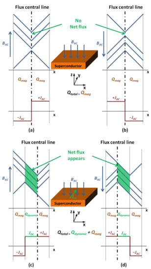
Figure 1.
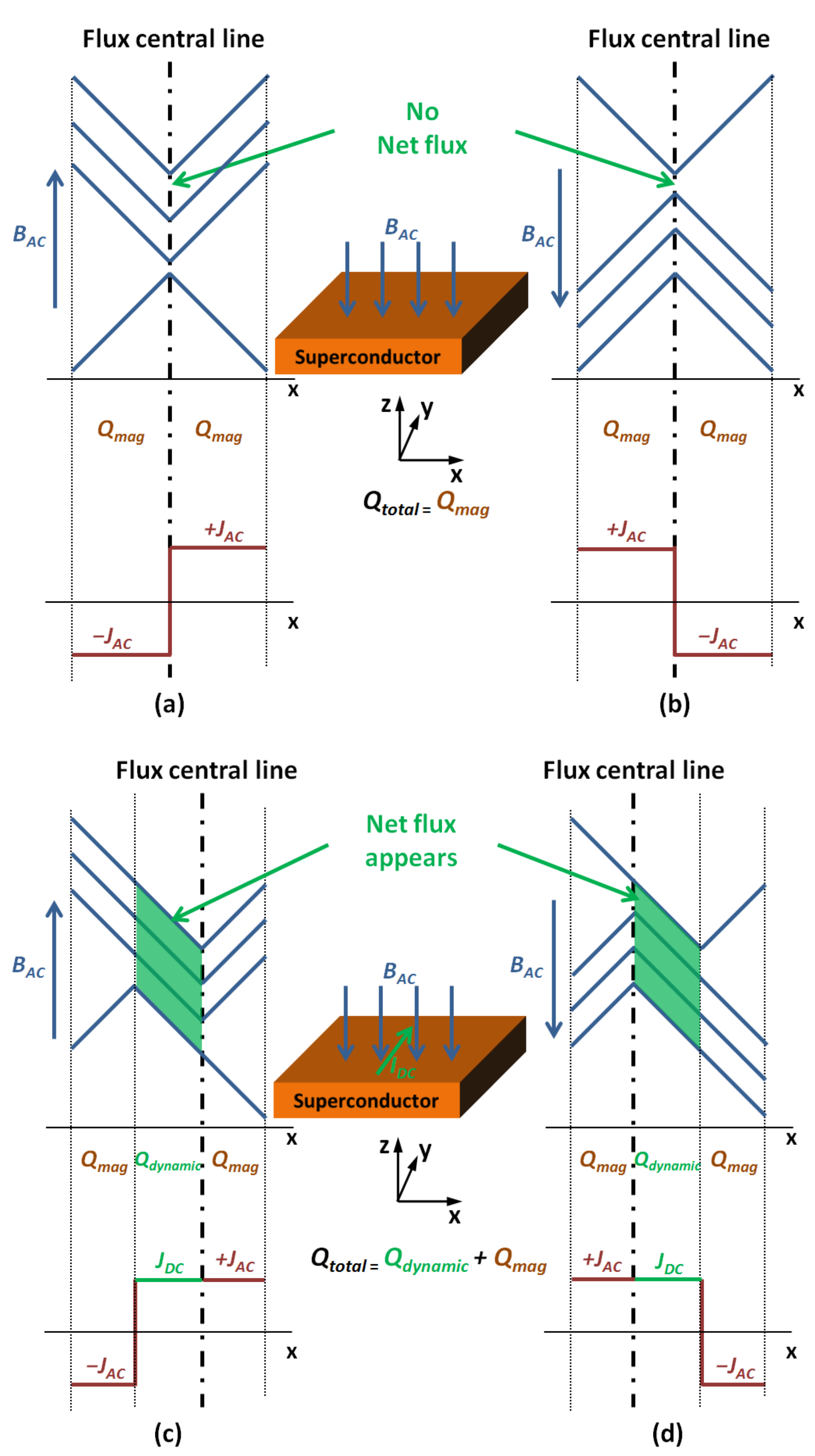
Bean model for a superconductor with an infinite length of height and depth (z direction and y direction) exposed to a perpendicular AC magnetic field, showing magnetic field and current profiles for (a,b): the original Bean model (no DC transport current), and (c,d): the Bean model with an extra DC transport current.
The original Bean model (no DC transport current) estimates the electromagnetic performance of a superconductor with an infinite length of height and depth (the z and y directions in Figure 1) exposed to a perpendicular AC magnetic field, and only the width of the superconductor is considered (the x direction in Figure 1). Consequently, the current profile in the x direction is negligible if compared to the y direction. An approximation can be made that induced currents only exist in the y direction (“+” or “−”, two-way).
For the Bean model in Figure 1a,b with no DC transport current in the y direction, as soon as the AC magnetic field starts increasing in the “+” cycle, screening currents JAC are induced in the two ends of the superconductor and progressively penetrate into the interior of the superconductor. When the AC magnetic field BAC hits its peak value that fully penetrates the superconductor, the screening currents JAC occupy the entire cross-section of the width (in Figure 1a, the x cross-section, either −JAC or +JAC). In Figure 1a,b, the slope is the derivative of the magnetic field inside the superconductor, whose value JAC is always equal to the superconducting critical current density:
In the “−” cycle (Figure 1b), when the BAC decreases by two times of the full penetration value, the current density profiles will be completely reversed (in Figure 1b, either +JAC or −JAC). After the entire cycle finishes, whilst the magnetic field profiles has been changing for the time being, the flux central line does not move during the whole cycle, and thus no net flux is induced. Accordingly, the total energy supplied by the system is merely converted to the magnetisation loss in the superconductor (Qtotal = Qmag).
For the Bean model with the addition of an extra DC transport current, as shown in the Figure 1c for the “+” cycle, the whole cross-section in the x direction is composed of three current elements (−JAC, JDC, and +JAC) when the BAC goes up to reach the peak value of full penetration, and, during this process, the flux central line shifts right to the border line between JDC and +JAC. Correspondingly, as shown in the Figure 1d for the “−” cycle, three current elements occupy the whole cross-section and are displayed in the sequence of +JAC, JDC, and −JAC when the BAC decreases by two times of the full penetration value, and during this process, the flux central line shifts left to the border line between +JAC and JDC. In the entire cycle, the flux central line shifts to the right border line and then shifts to the left border line, leading to a net flux ∆∅ in the middle of the superconductor:
where l and a are the length (y direction) and width (x direction) and of the superconductor, IDC is the DC transport current, Ic is the critical current, and BAC,th is the threshold field by which to achieve the full penetration of the superconductor. Based on Faraday’s law, the net flux ∆φ can induce a DC voltage that has an identical direction to that of the DC current in the superconductor, and is generally known as the dynamic voltage:
where f is the frequency of the AC magnetic field.
3. Modelling Method
In this study, the H-formulation incorporated into the FEM software COMSOL was used to simulate the phenomenon of superconducting dynamic voltage because the E-J power relation of the H-formulation is able to well present the superconducting characteristics, which are close to those of real superconducting behaviours and critical state models such as the Bean model.
The detailed derivation of the H-formulation has been presented in our previous work [29], whose core governing equation is:
where H is the magnetic field intensity, μ0 is the permeability of free space, μr is the relative permeability, and ρ is the resistivity of the material.
The critical current is an important variable used to determine the dynamic voltage. In order to model the accurate critical current of the HTS tape, a realistic critical current model of an anisotropic field was used to supplement the H-formulation:
where Bperp is the perpendicular magnetic flux density component to the wide surface of the HTS tape, and Bpara is the parallel magnetic flux density component to the wide surface of the HTS tape [30]. Table 1 presents the detailed parameters of the modelling method. Equations (4) and (5), as well as a collection of the electromagnetic equations, e.g., the Maxwell’s equations, were incorporated into the FEM software.

Table 1.
Parameters for the superconducting modelling.
The superconducting tape for modelling is a 4 mm HTS tape, with a critical current of Ic 100 A. Owing to the phenomenon of dynamic voltage only existing in the superconducting layer, other buffer layers and metal layers were ignored in this study. Only the 1 μm thick superconducting layer was studied in detail.
As shown in Figure 2, in order to verify the reliability of the modelling method, the current density pattern of the original Bean model and the reaction with an extra DC transport current was reproduced.
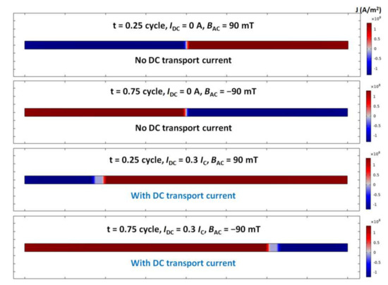
Figure 2.
“Original Bean model with no DC transport current” vs. “adjusted Bean model with an extra DC transport current of 0.3 Ic”: the current density distribution of a 4 mm HTS tape (the thickness was expanded by 100-fold, 100 μm, for better observation), perpendicularly exposed to a sinusoidal AC magnetic field (90 mT peak), at the time points of t = 1/4 cycle (BAC reached the positive maximum) and t = 3/4 cycle (BAC reached the negative maximum).
Figure 2 shows the comparison of the “original Bean model with no DC transport current” vs. the “adjusted Bean model with an extra DC transport current of 0.3 Ic”: the current density distribution of a 4 mm HTS tape (the thickness was expanded by 100-fold, 100 μm, for better observation), perpendicularly exposed to a sinusoidal AC magnetic field (90 mT peak), at the time points of t = 1/4 cycle (BAC reached the positive maximum) and t = 3/4 cycle (BAC reached the negative maximum). For the original Bean model without a DC transport current, Figure 2 shows the “+” and “−” current densities evenly distributed across the whole HTS tape, and the border line was in the centre of the HTS tape, which agreed with the typical Bean model patterns demonstrated in Figure 1a,b. For the adjusted Bean model with an extra DC transport current of 0.3 Ic, the “+” and “−” current densities were also distributed across the entire HTS tape; nevertheless, the border line between the “+” and “−” current densities was offset either to the left or right, and this phenomenon well matched the classic analytical solutions illustrated in Figure 1c,d.
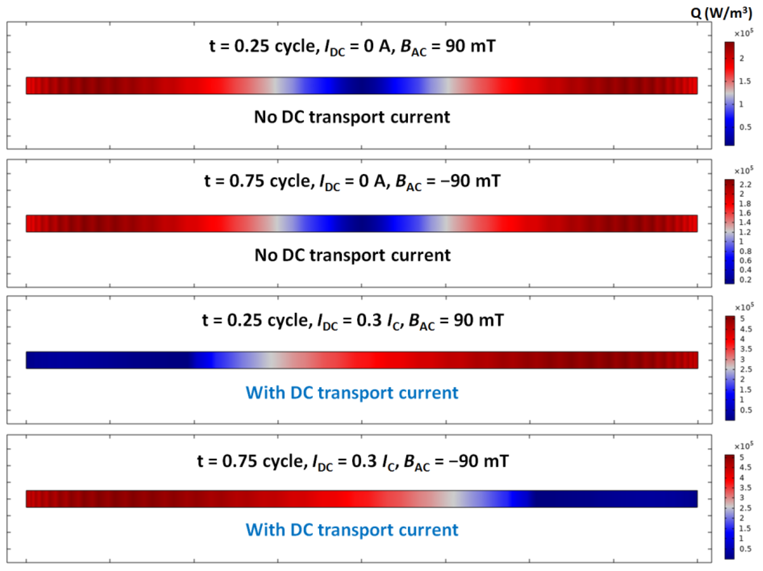
Figure 3 shows the instantaneous losses of a 4 mm HTS tape (corresponding to Figure 2), perpendicularly exposed to a sinusoidal AC magnetic field (90 mT peak), at the time points of t = 1/4 cycle (BAC reached the positive maximum) and t = 3/4 cycle (BAC reached the negative maximum), with or without a DC transport current. When there was no DC transport current, the loss pattern was symmetrical as the both the current distribution and voltage distribution were symmetrical in the HTS at t = 1/4 cycle or t = 3/4 cycle. However, with the DC transport current, the loss pattern was different, which was no longer symmetrical: strong on one side but weak on the other side. The reason was due to the amplitude of the voltage distribution being significantly weakened on the other side due to the compensation effect of the DC transport current.
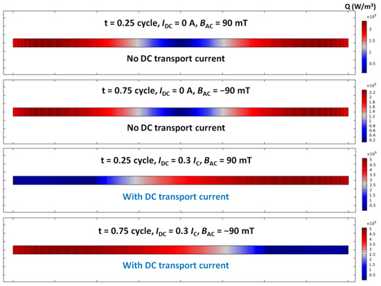
Figure 3.
Instantaneous losses of a 4 mm HTS tape (corresponding to Figure 2), perpendicularly exposed to a sinusoidal AC magnetic field (90 mT peak), at the time points of t = 1/4 cycle (BAC reached the positive maximum) and t = 3/4 cycle (BAC reached the negative maximum), with or without the DC transport current.
To summarise, the modelling method can well reproduce the analytical models. As it is very challenging to distinguish the total energy from the useful part and loss part by experiments, the modelling method could be the most suitable way by which to investigate the energy efficiency of the dynamic voltage characteristics of the HTS tape.
4. Optimisation of Energy Efficiency
After proving the reliability of the modelling method, more in-depth modelling was executed for this 4 mm HTS tape carrying different DC transport currents with different amplitudes and frequencies of the AC magnetic field.
Qdynamic is defined as the dynamic energy, which is equal to the dynamic voltage times the DC transport current:
Qdynamic can be a source of loss for a single (isolated) HTS tape within an AC magnetic field and with a DC transport current, and this energy will dissipate in the form of heat (similar to the AC loss). However, if this HTS tape is connected as a superconducting bridge into a flux pump, the energy Qdynamic can be regarded as the energy source that can charge the load of flux pump (useful energy). The total energy Qtotal is defined as the dynamic energy Qdynamic plus the magnetisation AC loss Qmag in the HTS tape:
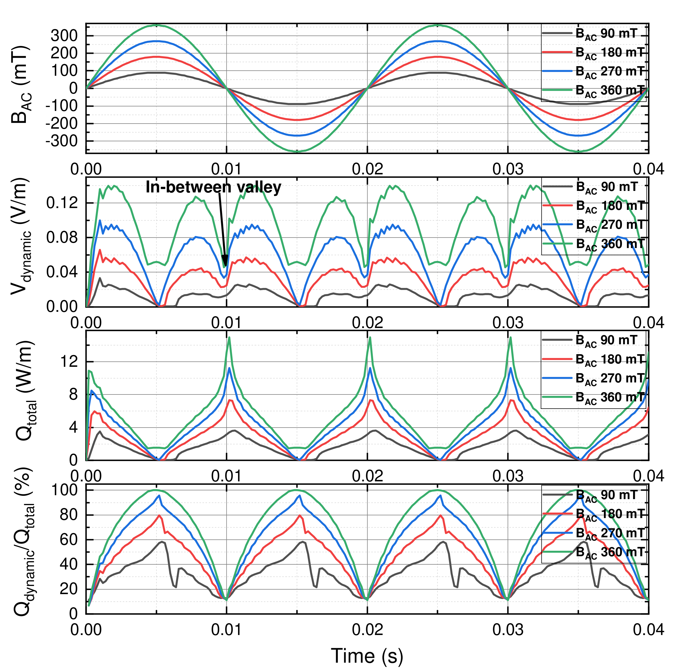
Figure 4 shows the instantaneous dynamic voltage, total energy Qtotal, and the Qdynamic/Qtotal ratio of a 4 mm HTS tape carrying DC transport currents at 30 A and exposed to different perpendicular 50 Hz sinusoidal AC magnetic fields, with peaks at 90 mT, 180 mT, 270 mT, and 360 mT. It can be seen that the frequency of the dynamic voltage was roughly two times the frequency of the applied AC magnetic field. The maximum instantaneous dynamic voltage occurred at every time after the AC magnetic field passed over the “0” point. The minimum instantaneous dynamic voltage happened around when the AC magnetic field reached the minimum or maximum and when the time derivative of the AC magnetic field was 0. As shown in the waveforms of Vdynamic, some “in-between valleys” appeared just before the magnetic field passed through the “0” point (e.g., around t = 0.0095 s). This phenomenon was more obvious when the magnetic fields increased to higher amplitudes, and potential reasons could be the magnetisation and that the interaction between the newly induced current and the residual current was more intense when the AC magnetic field reached higher amplitudes. The maximum total energy Qtotal happened approximately the same time as soon as the appearance of “in-between valleys”, which revealed that the magnetisation loss accounted for the majority at this moment as the “in-between valley” implied that the Qdynamic had a relatively low value. The Qdynamic/Qtotal ratio monotonically increased with the increasing AC magnetic field, which also agreed with the Equation (3). However, one important thing that should be carefully noted is that the Qdynamic/Qtotal reached 100% for around 1–1.5 ms with the AC magnetic field 360 mT case, which appeared abnormal as the AC loss could not be avoided when the superconductor was taking the AC current or AC magnetic field. Therefore, the reason for the Qdynamic taking 100% of the Qtotal could be that the superconductor had already been quenched with the 360 mT case, and the Qdynamic was no longer a normal energy of the dynamic voltage but a significant loss component. When the HTS tape was quenched within a higher magnetic field, the HTS tape was no longer superconducting but became very resistive, and the effect of superconducting magnetisation became much less significant. Therefore, at this moment, Qdynamic (the resistive component: the transport current times the voltage) dominated Qtotal, and the effect of the Qmag was negligible. This quench deduction can also be proved by the waveforms of Vdynamic and Qtotal with the 360 mT case always floating above 0 (even the minimum was over 0), while the other three normal cases always had minimum values touching down to 0.
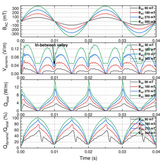
Figure 4.
Instantaneous dynamic voltage, total energy Qtotal, and the Qdynamic/Qtotal ratio of a 4 mm HTS tape carrying a DC transport current at 30 A, and exposed to different perpendicular 50 Hz sinusoidal AC magnetic fields, with peaks at 90 mT, 180 mT, 270 mT, and 360 mT.
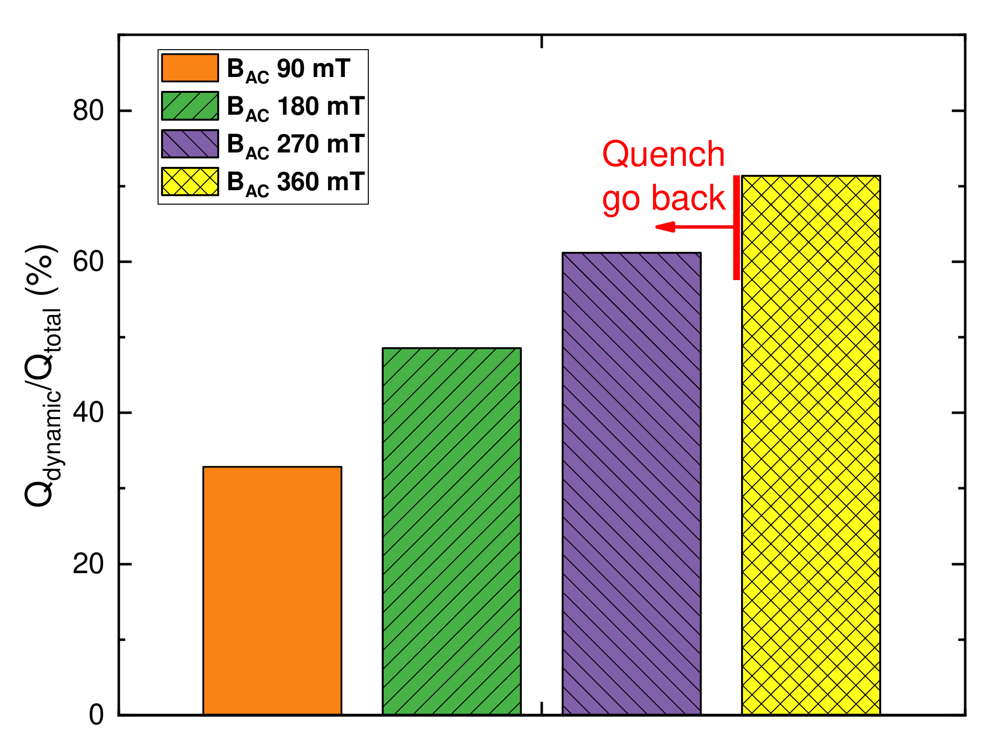
More straightforwardly, Figure 5 illustrates the average Qdynamic/Qtotal ratio for a whole cycle of a 4 mm HTS tape carrying 30 A DC transport currents and exposed to different perpendicular 50 Hz sinusoidal AC magnetic fields, with peaks at 90 mT, 180 mT, 270 mT, and 360 mT. Although the average Qdynamic/Qtotal ratio gradually increased from 32.9% to 71.4% as the AC magnetic fields’ peak increased from 90 mT to 360 mT, the 360 mT case was not valid for real applications because, at this time, the HTS tape had already become non-superconducting (quenched) and generated a considerable amount of loss and heat. Therefore, a lower Qdynamic/Qtotal ratio should be chosen before this point to ensure the safety for its use in real operations.
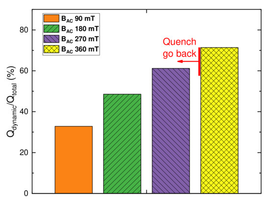
Figure 5.
Average Qdynamic/Qtotal ratio for a whole cycle of a 4 mm HTS tape carrying a 30 A DC transport current and exposed to different perpendicular 50 Hz sinusoidal AC magnetic fields, with peaks at 90 mT, 180 mT, 270 mT, and 360 mT.
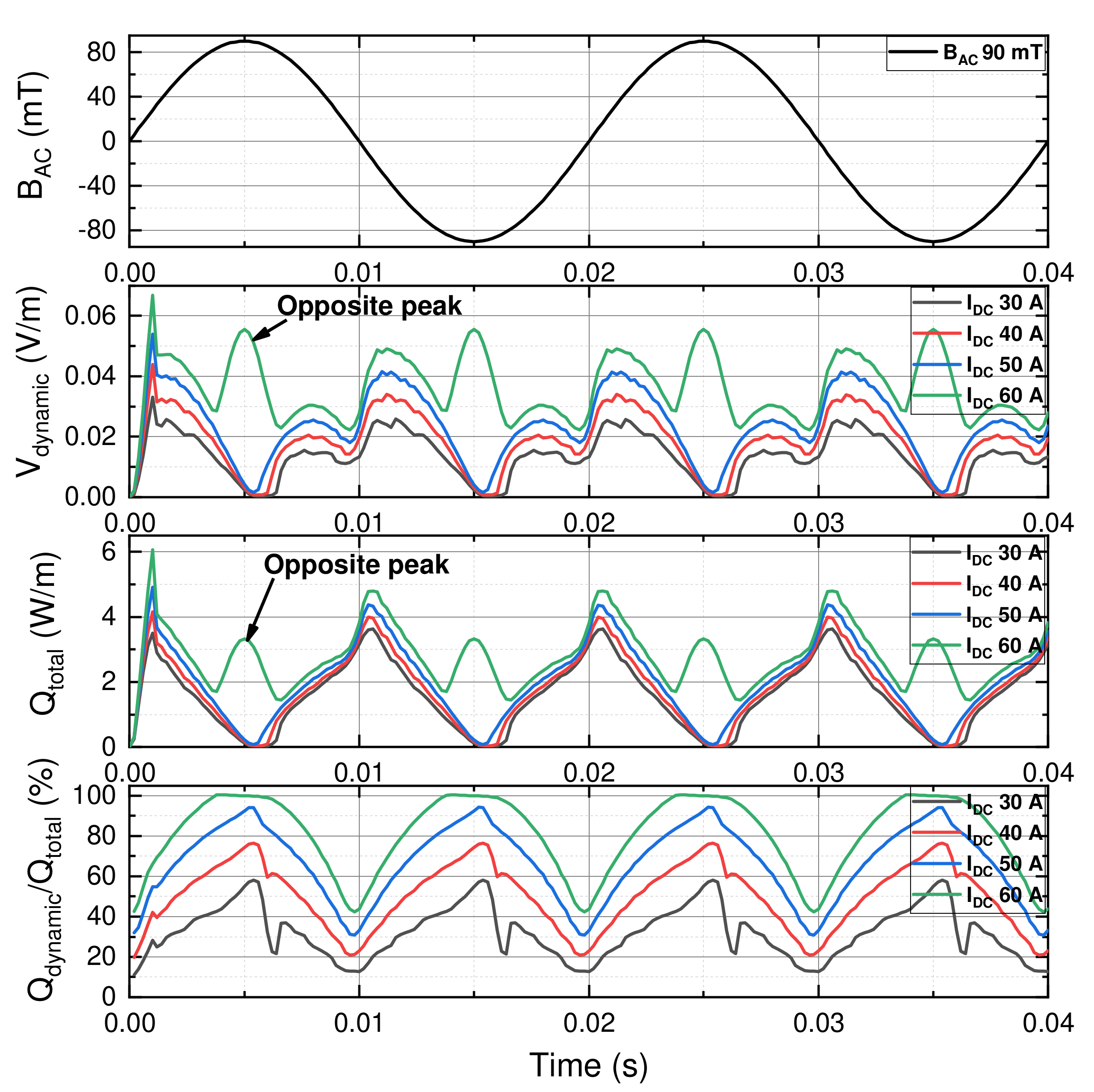
Figure 6 presents the instantaneous dynamic voltage, total energy Qtotal, and the Qdynamic/Qtotal ratio of a 4 mm HTS tape carrying different DC transport currents at 30 A, 40 A, 50 A, and 60, and exposed to a perpendicular 50 Hz sinusoidal AC magnetic field (90 mT peak). The overall shapes of dynamic voltage waveforms were similar to those of the dynamic voltage waveforms from the benchmarks with different AC magnetic fields, shown in Figure 4. However, the dynamic voltage waveform of the 60 A DC transport current case was different from those of the 30 A, 40 A, and 50 A cases: there were non-typical “opposite peaks” of the dynamic voltage waveforms in the 60 A case, which revealed that the 60 A case did not have the relaxation of the zero dynamic voltage or zero Qtotal. Additionally, the Qdynamic/Qtotal ratio also hit 100% for approximately 2–3 ms in duration around the time point when these “opposite peaks” of the dynamic voltage appeared. All of these occurrences implied that the quench could happen around the “opposite peaks” when the HTS tape was taking a 60 A DC transport current.
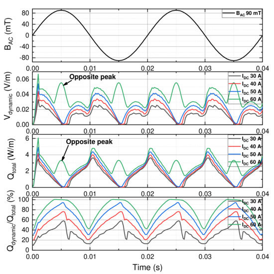
Figure 6.
Instantaneous dynamic voltage, total energy Qtotal, and the Qdynamic/Qtotal ratio of a 4 mm HTS tape carrying different DC transport currents (30 A, 40 A, 50 A, and 60 A) and exposed to a perpendicular 50 Hz sinusoidal AC magnetic field (90 mT peak).
Similar to Figure 5, Figure 7 demonstrates the average Qdynamic/Qtotal ratio for a whole cycle of a 4 mm HTS tape carrying different DC transport currents (30 A, 40 A, 50 A, and 60 A) and exposed to a perpendicular 50 Hz sinusoidal AC magnetic fields (90 mT peak). Obviously, the average Qdynamic/Qtotal ratio increased with the increasing amplitude of the DC transport current. The average Qdynamic/Qtotal ratio reached 81.8% in the case of DC transport currents of 60 A, but this did not necessarily mean that it achieved high energy efficiency because the HTS tape again had already been quenched and become resistive, and the Qdynamic at this time was not the useful energy but the energy loss. Consequently, a safe boundary of the Qdynamic/Qtotal ratio should be properly set for real operations.
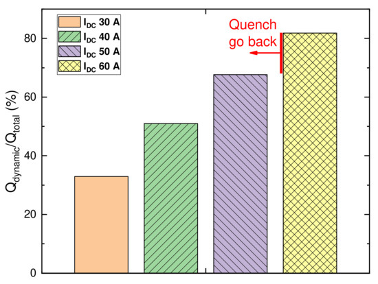
Figure 7.
Average Qdynamic/Qtotal ratio for a whole cycle of a 4 mm HTS tape carrying different DC transport currents (30 A, 40 A, 50 A, and 60 A) and exposed to a perpendicular 50 Hz sinusoidal AC magnetic field (90 mT peak).
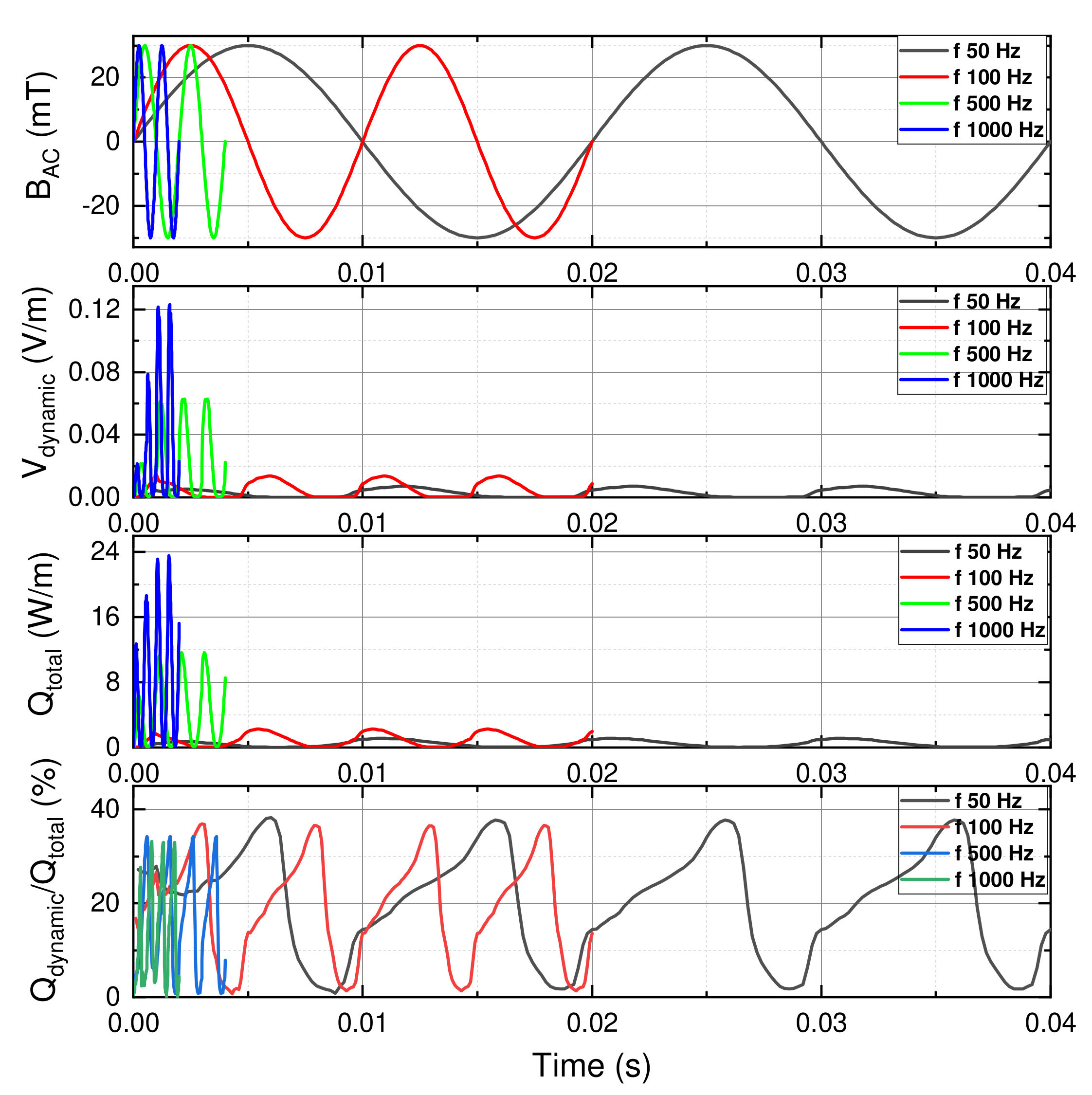
Figure 8 shows the instantaneous dynamic voltage, total energy Qtotal, and the Qdynamic/Qtotal ratio of a 4 mm HTS tape carrying a DC transport current at 30 A and exposed to the perpendicular sinusoidal AC magnetic fields, with the peak at 90 mT, at frequencies of 50 Hz, 100 Hz, 500 Hz, and 1000 Hz. It can be seen that both the amplitude and frequency of the instantaneous dynamic voltage had a linear correlation with the frequency of the AC magnetic field, which agreed well with the analytical solution in Equation (3). For example, the amplitude and frequency of the instantaneous dynamic voltage in the 1000 Hz case were both two times the amplitude and frequency of those in the 500 Hz case. The waveform patterns of Qtotal were fairly similar to the waveform patterns of Vdynalic, which also possessed a factor of two for the frequency. The situation of the Qdynamic/Qtotal waveforms with a wide range of frequencies was significantly different from the situations with different AC magnetic fields (Figure 4) and DC transport currents (Figure 6), where the Qdynamic/Qtotal ratio slightly decreased by 12.3% when the frequency greatly increased from 50 Hz to 1000 Hz, but maintained its level on the whole. If we do not consider the heat accumulation caused by the high-frequency magnetisation loss (discussed later), the higher operating frequency will not cause the quench of the HTS tape, which could be an advantage for high-frequency operations for dynamic voltage generation.
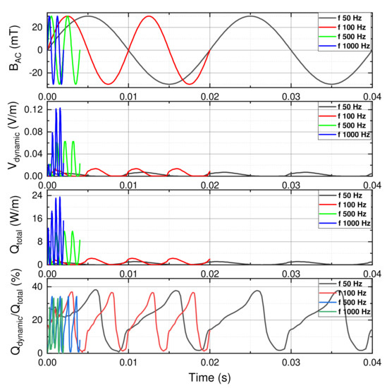
Figure 8.
Instantaneous dynamic voltage, total energy Qtotal, and the Qdynamic/Qtotal ratio of a 4 mm HTS tape carrying a DC transport current at 30 A and exposed to the perpendicular sinusoidal AC magnetic fields, with the peak at 90 mT, at frequencies at 50 Hz, 100 Hz, 500 Hz, and 1000 Hz.
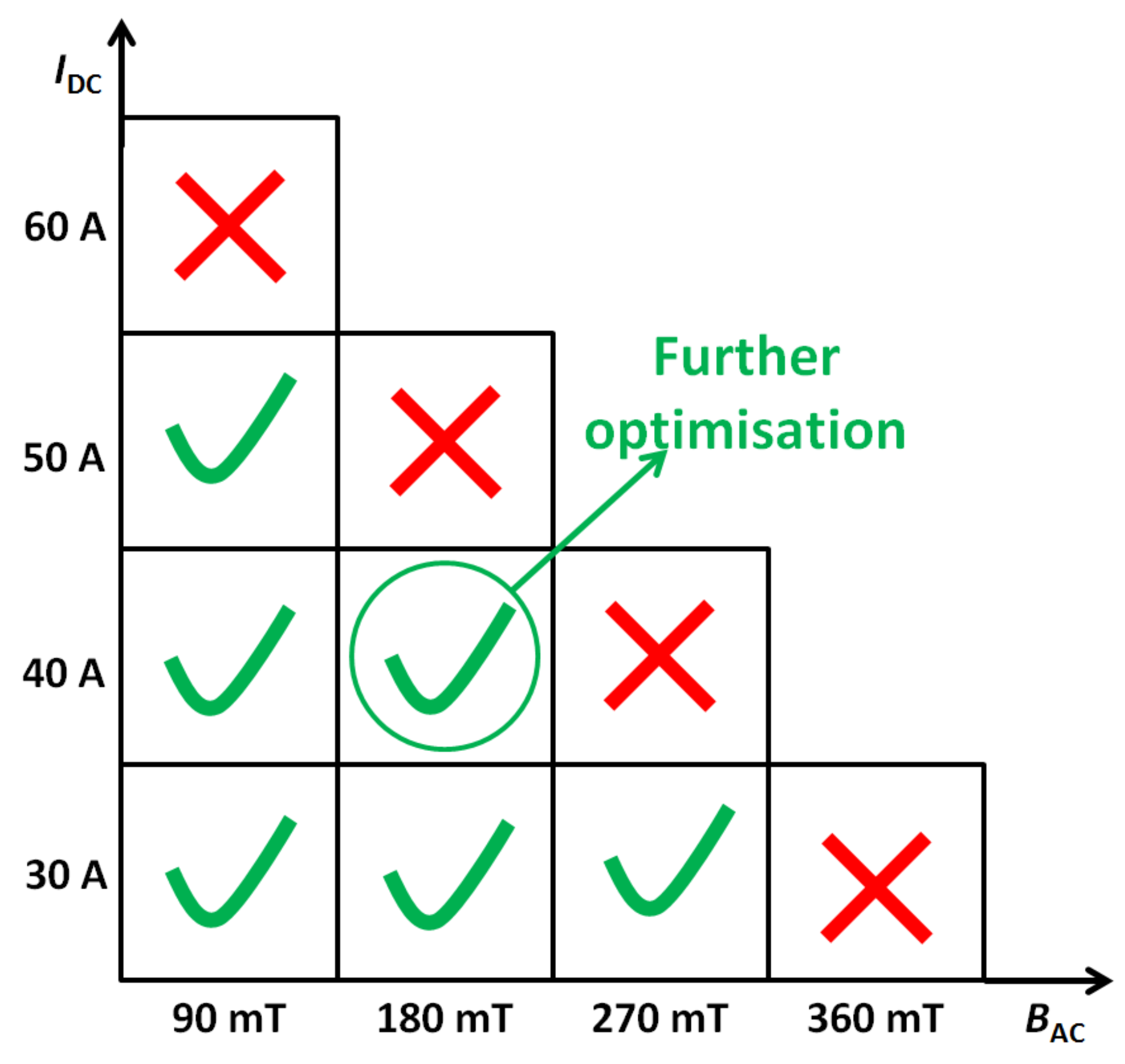
Based on the analysis from Figure 4, Figure 5, Figure 6, Figure 7 and Figure 8, some extreme cases briefly shaped the boundaries for safe operation, e.g., either the 4 mm HTS tape carrying a DC transport current at 30 A and exposed to an AC magnetic field with a 360 mT peak, or that carrying a DC transport current at 60 A and exposed to an AC magnetic field with a 90 mT peak. Figure 9 illustrates the strategy for further optimisation of the energy efficiency of dynamic voltage generated from a 4 mm HTS tape carrying a DC transport current and exposed to a perpendicular AC magnetic field, with the boundaries for safe operation. As shown in Figure 9, the cases with all the combinations of DC transport currents and AC magnetic fields were modelled one by one, and the successful cases (safe operation) and unsuccessful cases (unsafe operation) are marked in Figure 9. For example, the DC transport current of 50 A/AC with a magnetic field of 180 mT and the DC transport current of 40 A/AC with a magnetic field of 270 mT also quenched the HTS tape, while the DC transport current of 40 A/AC with a magnetic field of 180 mT were able to survive. Therefore, the DC transport current of 40 A/AC with a magnetic field of 180 mT was chosen as the candidate for further optimisation, and the “Nelder–Mead” optimisation tool embedded in COMSOL was used to further optimise the dynamic voltage and the energy efficiency with the constraints of safe operation (e.g., no quench).

Figure 9.
Strategy for further optimisation of the energy efficiency of dynamic voltage generated from a 4 mm HTS tape carrying a DC transport current and exposed to a perpendicular AC magnetic field, with the boundaries for safe operation.
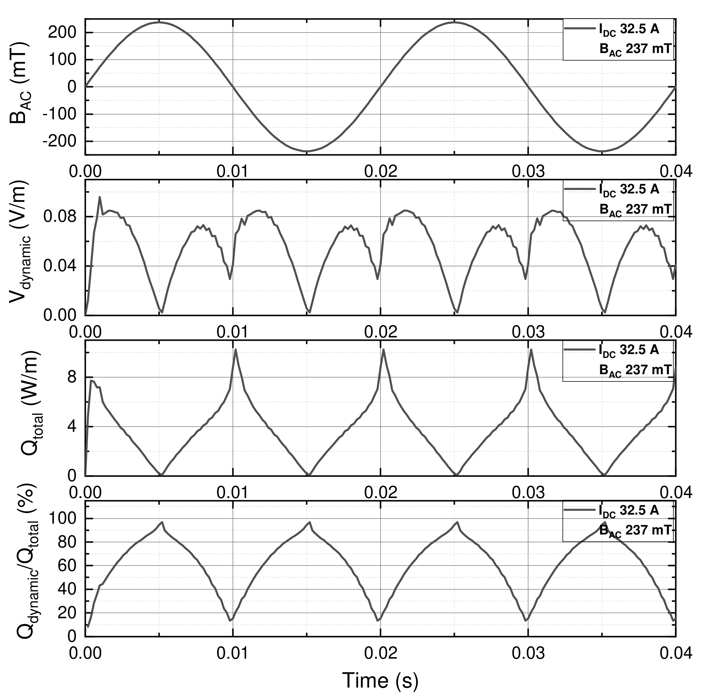
Figure 10 depicts the possible optimised case: the instantaneous dynamic voltage, total energy Qtotal, and the Qdynamic/Qtotal ratio of a 4 mm HTS tape carrying a DC transport current at 32.5 A and exposed to a sinusoidal AC magnetic field, with the peak at 237 mT. After the optimisation, the maximum instantaneous dynamic voltage was over 0.083 V/m, while the minimum dynamic voltage touched down to 0 V/m. There was no “opposite peak” in the waveforms of the dynamic voltage and Qtotal, and the Qtotal waveform had a minimum value close to zero. The peak of the Qdynamic/Qtotal waveform was over 95% but never reached the 100% line. All this evidence could prove that the HTS tape operated in the superconducting state (no quench) and within the safe region, and with a reasonably high energy efficiency.
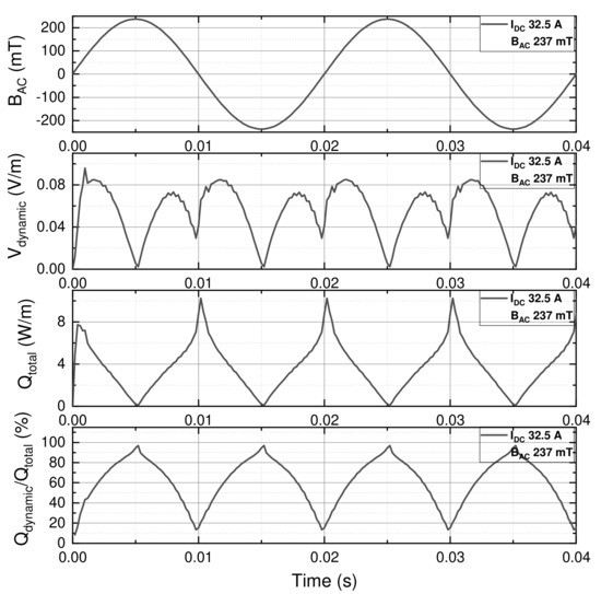
Figure 10.
Possible optimised case: the instantaneous dynamic voltage, total energy Qtotal, and the Qdynamic/Qtotal ratio of a 4 mm HTS tape carrying a DC transport current at 32.5 A and exposed to a sinusoidal AC magnetic field, with the peak at 237 mT.
Having properly optimised the DC transport current and AC magnetic field to generate the dynamic voltage with a good energy efficiency, the proper operating frequency of the AC magnetic field should be chosen. As mentioned above, the operating frequency was linearly correlated with the dynamic voltage, which should be ideally as high as possible. The frequency of the AC magnetic field did not lead to the quench of the HTS directly, but the corresponding magnetisation loss (in Watts) increased with the increasing frequency, and the accumulated heat could probably have caused the quench of the HTS tape. In general, the operating frequency is largely dependent on the cooling approaches, material composition, and the geometry of the superconducting devices. For a small-to-medium scale HTS flux pump, the operating frequency could be chosen from 20 Hz to 2000 Hz.
5. Conclusions
This article has explored the energy efficiency optimisation of dynamic voltage in an HTS tape taking different DC transport currents and exposed to different AC magnetic fields. In the beginning, the fundamental physics of the superconducting dynamic voltage were explained using the Bean model and classic analytical solutions. The modelling method was based on the H-formulation merged into the FEM software, COMSOL, whose feasibility was verified by reproducing the typical behaviours of the Bean model and the analytical solutions of the dynamic voltage. Comprehensive simulations were executed to optimise the energy efficiency regarding the dynamic voltage in a 4 mm HTS tape taking DC transport currents from 30 A to 60 A, AC magnetic field magnitudes from 90 mT to 360 mT, and frequencies from 50 Hz to 1000 Hz. Due to the physical constraints of the HTS tape (e.g., quench), a safe operating region was defined. A more accurate optimisation was carried to explore the optimal operating conditions: a DC transport current at 32.5 A and an AC magnetic field with a peak at 237 mT, where both a reasonable dynamic voltage and energy efficiency can be achieved for the HTS tape. It should be noted that eddy currents can be induced in the metal layers (e.g., copper stabilisers and silver over-layers) and interact with the superconducting layer, particularly for high-frequency operation. Future works such as an eddy-current analysis and a comprehensive thermo-coupled model can be established to make more realistic designs and optimisations. In this article, the optimisation approach, analysis, and results of the study of superconducting dynamic voltage are useful for the future design and optimisation of superconducting energy/power devices under complex electromagnetic conditions.
Author Contributions
Conceptualisation, B.S.; methodology, B.S. and X.C.; software, B.S. and L.F.; validation, B.S., X.C., and M.Z.; formal analysis, B.S. and M.Z.; investigation, B.S. and L.F.; resources, B.S. and X.B.; data curation, B.S.; writing—original draft preparation, B.S. and L.F.; writing—review and editing, L.F. and X.C.; visualisation, B.S.; supervision, B.S. and X.C.; project administration, B.S. and X.B.; funding acquisition, B.S. and X.B. All authors have read and agreed to the published version of the manuscript.
Funding
This work was in part supported by the State Key Laboratory of Alternate Electrical Power System with Renewable Energy Sources (Grant No. LAPS22008).
Data Availability Statement
The data presented in this study are available on request from the corresponding author.
Acknowledgments
The authors would like to thank T. Coombs from the University of Cambridge, UK, for the useful comments.
Conflicts of Interest
The authors declare no conflict of interest.
References
- Alam, M.S.; Alotaibi, M.A.; Alam, M.A.; Hossain, M.A.; Shafiullah, M.; Al-Ismail, F.S.; Rashid, M.M.U.; Abido, M.A. High-Level Renewable Energy Integrated System Frequency Control with SMES-Based Optimized Fractional Order Controller. Electronics 2021, 10, 511. [Google Scholar] [CrossRef]
- Stephan, R.M.; Pereira, A.O., Jr. The Vital Contribution of MagLev Vehicles for the Mobility in Smart Cities. Electronics 2020, 9, 978. [Google Scholar] [CrossRef]
- Chen, X.; Chen, Y.; Zhang, M.; Jiang, S.; Gou, H.; Pang, Z.; Shen, B. Hospital-oriented quad-generation (hoqg)—A combined cooling, heating, power and gas (cchpg) system. Appl. Energy 2021, 300, 117382. [Google Scholar] [CrossRef]
- Chen, X.; Xie, Q.; Bian, X.; Shen, B. Energy-saving superconducting magnetic energy storage (smes) based interline dc dynamic voltage restorer. CSEE J. Power Energy Syst. 2022, 8, 238–248. [Google Scholar] [CrossRef]
- Noe, M.; Steurer, M. High-temperature superconductor fault current limiters: Concepts, applications, and development status. Supercond. Sci. Technol. 2007, 20, R15–R29. [Google Scholar] [CrossRef]
- Chen, X.; Gou, H.; Chen, Y.; Jiang, S.; Zhang, M.; Pang, Z.; Shen, B. Superconducting fault current limiter (sfcl) for a power electronic circuit: Experiment and numerical modelling. Supercond. Sci. Technol. 2022, 35, 045010. [Google Scholar] [CrossRef]
- Shen, B.; Chen, Y.; Li, C.; Wang, S.; Chen, X. Superconducting fault current limiter (sfcl): Experiment and the simulation from finite-element method (fem) to power/energy system software. Energy 2021, 234, 121251. [Google Scholar] [CrossRef]
- Ko, S.-C.; Han, T.-H.; Lim, S.-H. DC current limiting operation and power burden characteristics of a flux-coupling type sfcl connected in series between two windings. Electronics 2021, 10, 1087. [Google Scholar] [CrossRef]
- Uglietti, D. A review of commercial high temperature superconducting materials for large magnets: From wires and tapes to cables and conductors. Supercond. Sci. Technol. 2019, 32, 053001. [Google Scholar] [CrossRef]
- Chen, X.; Jiang, S.; Chen, Y.; Zou, Z.; Shen, B.; Lei, Y.; Zhang, D.; Zhang, M.; Gou, H. Energy-saving superconducting power delivery from renewable energy source to a 100-mw-class data center. Appl. Energy 2022, 310, 118602. [Google Scholar] [CrossRef]
- Parizh, M.; Lvovsky, Y.; Sumption, M. Conductors for commercial mri magnets beyond nbti: Requirements and challenges. Supercond. Sci. Technol. 2016, 30, 014007. [Google Scholar] [CrossRef] [PubMed] [Green Version]
- Chen, X.; Jiang, S.; Chen, Y.; Lei, Y.; Zhang, D.; Zhang, M.; Gou, H.; Shen, B. A 10 mw class data center with ultra-dense high-efficiency energy distribution: Design and economic evaluation of superconducting dc busbar networks. Energy 2022, 123820. [Google Scholar] [CrossRef]
- Shen, B.; Grilli, F.; Coombs, T. Review of the ac loss computation for hts using h formulation. Supercond. Sci. Technol. 2020, 33, 033002. [Google Scholar] [CrossRef] [Green Version]
- Shen, B.; Li, C.; Geng, J.; Zhang, X.; Gawith, J.; Ma, J.; Liu, Y.; Grilli, F.; Coombs, T.A. Power dissipation in hts coated conductor coils under the simultaneous action of ac and dc currents and fields. Supercond. Sci. Technol. 2018, 31, 075005. [Google Scholar] [CrossRef]
- Oomen, M.; Rieger, J.; Leghissa, M.; ten Haken, B.; ten Kate, H.H. Dynamic resistance in a slab-like superconductor with jc (b) dependence. Supercond. Sci. Technol. 1999, 12, 382–387. [Google Scholar] [CrossRef]
- Brandt, E.H.; Mikitik, G.P. Why an ac magnetic field shifts the irreversibility line in type-ii superconductors. Phys. Rev. Lett. 2002, 89, 027002. [Google Scholar] [CrossRef] [Green Version]
- Ogasawara, T.; Yasuköchi, K.; Nose, S.; Sekizawa, H. Effective resistance of current-carrying superconducting wire in oscillating magnetic fields 1: Single core composite conductor. Cryogenics 1976, 16, 33–38. [Google Scholar] [CrossRef]
- Geng, J.; Matsuda, K.; Fu, L.; Shen, B.; Zhang, X.; Coombs, T. Operational research on a high-tc rectifier-type superconducting flux pump. Supercond. Sci. Technol. 2016, 29, 035015. [Google Scholar] [CrossRef]
- Ainslie, M.D.; Bumby, C.W.; Jiang, Z.; Toyomoto, R.; Amemiya, N. Numerical modelling of dynamic resistance in high-temperature superconducting coated-conductor wires. Supercond. Sci. Technol. 2018, 31, 074003. [Google Scholar] [CrossRef]
- Hu, J.; Ma, J.; Yang, J.; Tian, M.; Shah, A.; Patel, I.; Wei, H.; Hao, L.; Ozturk, Y.; Shen, B.; et al. Numerical study on dynamic resistance of an hts switch made of series-connected ybco stacks. IEEE Trans. Appl. Supercond. 2021, 31, 8200106. [Google Scholar] [CrossRef]
- Li, C.; Xing, Y.; Yang, J.; Guo, F.; Li, B.; Xin, Y.; Shen, B. The instantaneous dynamic resistance voltage of dc-carrying rebco tapes to ac magnetic field. Phys. C Supercond. 2021, 583, 1353853. [Google Scholar] [CrossRef]
- Sun, Y.; Fang, J.; Sidorov, G.; Li, Q.; Badcock, R.A.; Long, N.J.; Jiang, Z. Total loss measurement and simulation in a rebco coated conductor carrying dc current in perpendicular ac magnetic field at various temperatures. Supercond. Sci. Technol. 2021, 34, 065009. [Google Scholar] [CrossRef]
- Zhang, H.; Chen, H.; Jiang, Z.; Yang, T.; Xin, Y.; Mueller, M.; Li, Q. A full-range formulation for dynamic loss of high-temperature superconductor coated conductors. Supercond. Sci. Technol. 2020, 33, 05LT01. [Google Scholar] [CrossRef]
- Zhang, H.; Yao, M.; Jiang, Z.; Xin, Y.; Li, Q. Dependence of dynamic loss on critical current and n-value of hts coated conductors. IEEE Trans. Appl. Supercond. 2019, 29, 8201907. [Google Scholar] [CrossRef] [Green Version]
- Jiang, Z.; Hamilton, K.; Amemiya, N.; Badcock, R.; Bumby, C. Dynamic resistance of a high-tc superconducting flux pump. Appl. Phys. Lett. 2014, 105, 112601. [Google Scholar] [CrossRef]
- Jiang, Z.; Toyomoto, R.; Amemiya, N.; Bumby, C.W.; Badcock, R.A.; Long, N.J. Dynamic resistance measurements in a gdbco-coated conductor. IEEE Trans. Appl. Supercond. 2016, 27, 5900205. [Google Scholar] [CrossRef]
- Jiang, Z.; Zhou, W.; Li, Q.; Yao, M.; Fang, J.; Amemiya, N.; Bumby, C.W. The dynamic resistance of ybco coated conductor wire: Effect of dc current magnitude and applied field orientation. Supercond. Sci. Technol. 2018, 31, 035002. [Google Scholar] [CrossRef] [Green Version]
- Bean, C.P. Magnetization of hard superconductors. Phys. Rev. Lett. 1962, 8, 250–253. [Google Scholar] [CrossRef]
- Shen, B.; Grilli, F.; Coombs, T. Overview of h-formulation: A versatile tool for modelling electromagnetics in high-temperature superconductor applications. IEEE Access 2020, 8, 100403–100414. [Google Scholar] [CrossRef]
- Chen, X.; Pang, Z.; Gou, H.; Xie, Q.; Zhao, R.; Shi, Z.; Shen, B. Intelligent design of large-size hts magnets for smes and high-field applications: Using a self-programmed gui tool. Supercond. Sci. Technol. 2021, 34, 095008. [Google Scholar] [CrossRef]


Publisher’s Note: MDPI stays neutral with regard to jurisdictional claims in published maps and institutional affiliations. |
© 2022 by the authors. Licensee MDPI, Basel, Switzerland. This article is an open access article distributed under the terms and conditions of the Creative Commons Attribution (CC BY) license (https://creativecommons.org/licenses/by/4.0/).