A Maritime Traffic Network Mining Method Based on Massive Trajectory Data

Abstract

Intelligent ships are the future direction of maritime transportation. Route design and route planning of intelligent ships require high-precision, real-time maritime traffic network information, which changes dynamically as the traffic environment changes. At present, there is a lack of high-precision and accurate information extraction methods for maritime traffic networks. Based on the massive trajectory data of vessels, the adaptive waypoint extraction model (ANPG) is proposed to extract the critical waypoints on the traffic network, and the improved kernel density estimation method (KDE-T) is constructed to mine the spatial–temporal characteristics of marine lanes. Then, an automatic traffic network generation model (NNCM), based on the pix2pix network, is put forward to reconstruct the maritime traffic network. NNCM has been tested on the historical trajectory data of Humen waters and Dongping waters in China, the experimental results show that the NNCM model improves the extraction accuracy by 13% and 33% compared to the geometric analysis method and density clustering method. It is of great significance to improve the navigation accuracy of intelligent ships. This method can also provide important technical support for waterway design and monitoring and maritime traffic supervision.

1. Introduction

Unmanned surface vessels are the future direction of maritime transportation [1,2]. The key technologies of intelligent vessels, such as maritime voyage planning, ship navigation, and digital waterway, require high-precision, real-time digital maritime traffic network information as the data basis and technical support [3]. Hence, the method for extraction of maritime traffic networks with good stability and high precision is of great significance to improve the intelligence level of vessels, promote the construction of digital channels, and ensure the safety of navigation. Different from the road network, the maritime traffic network changes dynamically, due to the influence of factors such as the traffic environment, hydrometeorological conditions, seasonal time, and shipping economic development, which brings great difficulties for extracting maritime traffic networks.

In the current research, the structure of the route network extraction method can be divided into two parts: One part constructs the navigation area through the geometric method. The geometric method considers the spatial characteristics of all ship trajectories and can reconstruct the route network in restricted waters. However, the result can only provide a rough reference for ship navigation safety and path planning. In addition, this method is easily disturbed by outliers. The limitations lead to poor accuracy in complex waters. The other part analyzes the semantic information of the ship trajectory by means of clustering algorithms, which mine potential ship maneuvering points and connect them to generate a route network. The points are beneficial to improve the practicability of the route network structure. However, it is difficult for the clustering algorithms to mine and analyze a large amount of data due to the complexity of the calculation. At the same time, the real navigation environment is dynamic and cannot be described by a single mathematical formula. Existing studies still have various problems in adapting to large-scale sea areas, the complexity of the navigation environment, and existing traffic patterns. Ship trajectory data contain rich potential laws [4,5] and have not been fully exploited and applied.

To overcome these defects, the study aims to detect the spatial–temporal properties of trajectories to construct a new maritime traffic network extraction method. The main contributions of this study are as follows: (1) In order to capture the potential feature of ships and traffic, a trajectory kernel density estimation method suitable for ship characteristics is designed, so as to realize the extraction of ship experience routes. (2) In view of the dynamic characteristics of the maritime traffic network, our approach calculates the course and cumulative volume of local ship traffic and avoids the use of uniform thresholds, which achieves a higher integrity. (3) For adapting to a large range of complex waters, the study proposes the use of conditional generative adversarial networks (CGANs) to solve the generation problem of the route network. Benefiting from the excellent expression ability of deep learning, the accuracy and robustness of the method were greatly improved.

2. Related Work

In general, the maritime traffic network and route extraction methods include grid-based methods, vector-based methods, and statistical methods. A grid-based method constructs the original traffic data within a set of index grids [3]. Maritime routes are more likely discovered in dense areas. Wang et al. [6] proposed a parallel grid merging and filtering algorithm based on Quad-Trees. Delaunay triangulation was applied to extract route boundary information. However, abnormal data have a great influence on the results. Lu et al. [7] used kernel density estimate (KDE) to infer the edge of the route and constructed popular routes through triangulation. A vector method establishes a traffic network by extracting waypoints. Tang et al. [8] designed a heading criterion and topology extraction method to derive topology points. To model the maritime traffic state, cluster algorithms [9], such as prototype-based clustering [10,11,12], density-based clustering [13], and hierarchical clustering, are suitable for mining and analyzing sampling points. Arguedas et al. [14] proposed an inner and outer traffic network to solve the accuracy problem. Edelkamp [15] applied the K-means algorithm to cluster the trajectory points. Based on the distance and direction, they adopted a suitable spline curve to simulate the centerline. Jin et al. [16] proposed adaptive density incremental clustering to extract frequent trajectories. Wang et al. [17] applied density-based spatial clustering to form different trajectory vector clusters and proposed adding vessel heading and course to ground and trajectory coordinates to form 3D spherical coordinates to extract the centerline to construct a traffic network. However, with these methods, it is hard to process big data because of the requisite huge amounts of calculations. The statistical method is a combination of digital image processing [18] technology, a clustering algorithm, and GIS technology to extract route features. It focuses on a statistical analysis of maritime routes [3]. Yan et al. [19] transformed ship trajectory into ship navigation semantic behavior (STSO). Based on graph theory, STSO was integrated into the topological structure with a maritime traffic graph to realize the extraction and expression of shipping routes. Filipiak et al. [20] constructed a directed graph by combining a spatial index and genetic algorithm (GA) [21] to extract waypoint information, which can reflect the real sea route, but the graph was too redundant. Lee et al. [22] combined the python image processing technology with KDE to complete route extraction. This method requires manual intervention and performs poorly in extracting routes at intersections. To solve the problems of low quality of trajectory data and non-uniform sampling, Wang et al. [23] regarded trajectory as terrain elevation to achieve road network reconstruction. Nicola et al. [24] extended the traffic flow theory to construct an undirected graph of a route, but it could not guide the actual navigation and route planning of the ship.

Although those studies made important achievements in maritime traffic network reconstruction, there are still limitations in two aspects. On the one hand, the waypoint detection algorithms are mostly mined by the density of trajectory points, and the extraction results are concentrated on cross routes and narrow routes. In practice, the density distribution of the trajectory points is quite uneven in different areas [6]. On the other hand, the existing methods apply topology and geometry methods to solve the problem of waypoint connections. The generated traffic network has overlapping, missing, and abnormal edges. To resolve errors, specific optimization processing operations are desired for the spatial–temporal characteristics of the data.

3. System Model and Definition

As Figure 1 shows, an automatic identification system (AIS) can work continuously when the ship is sailing or berthing, broadcast the navigation information to other devices, and effectively transmit the navigation data between ships and shore stations. AIS data contain four different types of information: dynamic information, static information, navigation-related information, and safety-related information. Considering the need for dynamic information and static information, this study selects the Maritime Mobile Packet Service Identity (MMSI), longitude, latitude, etc., as shown in

Table 1. An overview of AIS data.

MMSI	Length (m)	Width (m)	Draught (m)	Longitude (°)	Latitude (°)	Speed (kn)	Course (°)	Time
413xxx062	67	21	7	112.86136	23.2863	5.5	192.5	01:43:24
413xxx062	67	21	7	112.86002	23.2826	5.5	203.1	01:45:52
413xxx062	67	21	7	112.85786	23.2792	5.5	221.0.1	01:48:25

.

As presented in Figure 1 and Table 1, the AIS data can be regarded as time-series data, and the changes in value are relatively stable. At points P1, P2, P3, P4, and P5 of Figure 1, there are obvious changes in the courses of vessels, indicating that the vessels had performed steering maneuvers. If multiple vessels choose the same area to turn, this area may be an important waypoint. At the same time, the navigation areas of most ships can represent the route. The structure of the maritime traffic is composed of nodes (P1, P2, P3, P4, P5) and edges (W1, W2, W3, W4). In shape, nodes are waypoints, and edges are connections of the node’s shortest route.

This study design utilizes the longitude $lon$, latitude $lat$, speed over ground $v$, course over ground $c$, and length of ship $l$ recorded by AIS data to build a maritime traffic network extraction model. The model input $X$ is the sequence of $n$ ship trajectories in time interval $t$:

$$X=\left(X_1,X_2,\dots ,X_n\right), X_i=\left(x_1,x_2,\dots x_t\right), x_{ii}=\left(lon,lat,v,c,l\right)$$

(1)

A maritime traffic network can be constructed by the graph data structure. In Equation (2), graph $Z$ consists of nodes $P$ and edges $W$. The nodes are the actual waypoints in marine traffic. The number of $P$ is $r$ (Equation (3)). Each node $p$ includes longitude $p_x$ and latitude $p_y$. In Equation (4), the number of $W$ is $m$. Each edge $w$ represents a route between nodes $p_h$ and $p_j$, where $h$ is not equal to $j$. In addition, a Boolean value $E{D}_{hj}$ is used to judge whether node $p_h$ can directly reach node $p_j$ without passing through any node. In Equation (5), $O$ represents the rasterized traffic environment; the size is $u$; and each grid has three attributes of abscissa $o_x$, ordinate $o_y$, and trajectory density value $density$.

$$Z=\left(P,W\right)$$

(2)

$$P=\left(p_1,p_2,\dots ,p_r\right), p_i=\left(p_x,p_y\right)$$

(3)

$$W=\left(w_1,w_2,\dots ,w_m\right),\hspace{1em}{w}_i=\left(p_h,p_j,E{D}_{hj}\right)$$

(4)

$$O=\left(o_1,o_2,\dots ,o_u\right),\hspace{1em}{o}_i=(o_x,o_y,density)$$

(5)

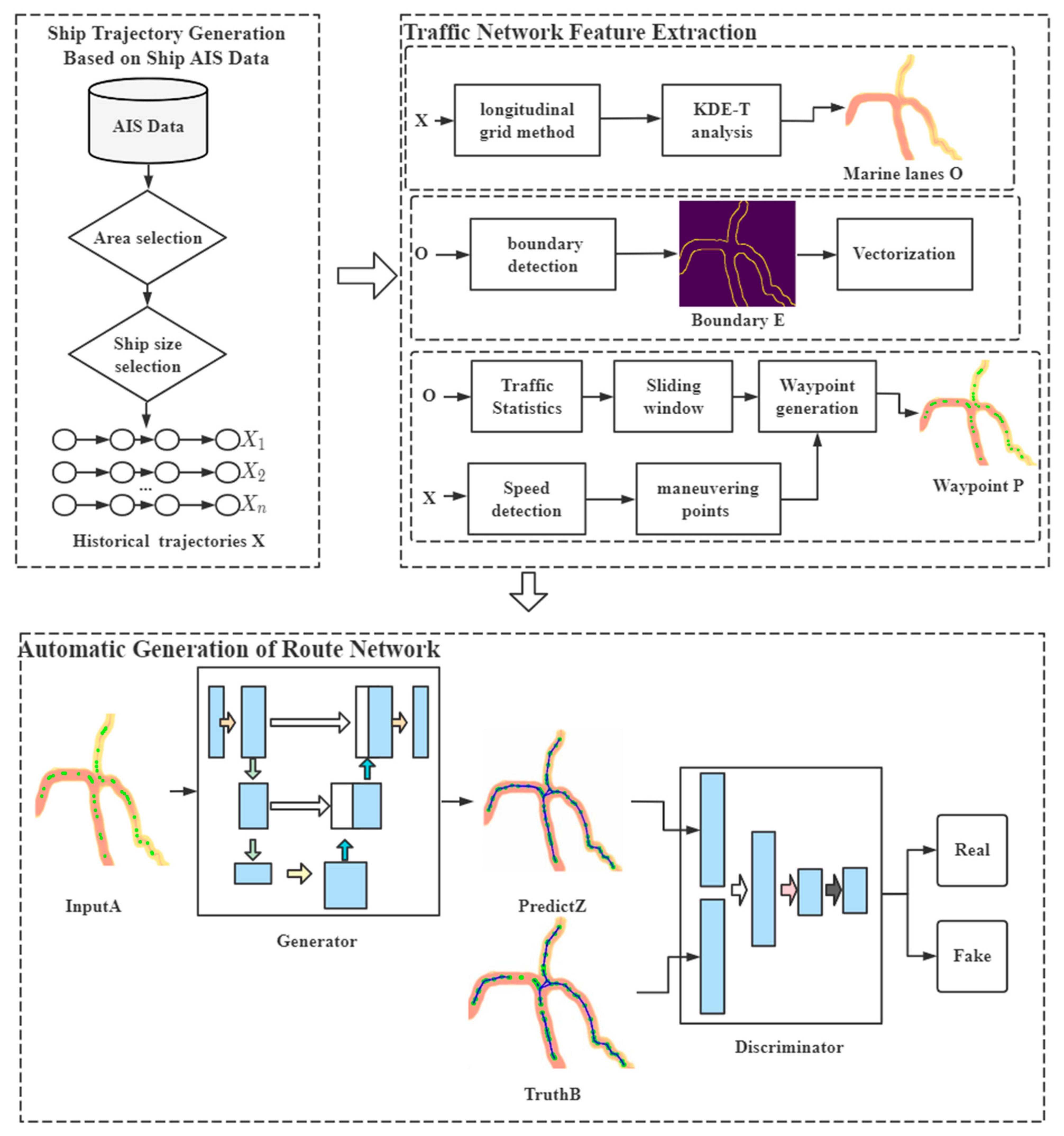
4. Our Proposed Maritime Traffic Network Extraction Scheme

The relevant methods in this study are KDE and pix2pix: KDE is a spatial analysis of point events, focusing on the underlying properties of point events and measuring variation in the mean value of the process. The KDE algorithm has been widely used in the analysis and detection of “hotspots” in the traffic environment. Pix2pix is based on the CGAN architecture, which performs well in the task of image-to-image translation. The generator consists of a U-Net structure suitable for processing images whose input and output share the same underlying structure. The discriminator is composed of a fully convolutional network, which can better judge the local part of the image.

As illustrated in Figure 2, the structure of the maritime traffic network extraction can be divided into three essential parts: ship trajectory generation, traffic network feature extraction, and traffic network automatic generation. Firstly, the ship trajectory generation module preprocesses massive AIS data and generates ship trajectory data $X$. Secondly, the traffic network feature extraction module establishes extraction methods for the constituent elements of the traffic network, including waypoints, marine lane boundaries, and lanes. Through KDE-T analysis, the trajectory $X$ is converted into a grid of marine lanes. Then, boundary detection extracts marine lane boundaries. In this situation, the waypoint extraction model considers the statistics of traffic flow and searches for the maximum of local adjacency points. However, because too many waypoints will increase the redundancy of the network [25,26], the model detects vessel maneuvering points to filter the results. Finally, the automatic generation module of the traffic network realizes the automatic matching of the elements, reconstructing the maritime traffic network rapidly. It is mainly made up of a generator and a discriminator. The input of the generator is the traffic network features. The features are continuously passed down through skip connections to retain as much feature information as possible. Designed in the form of a fully convolutional network, the discriminator takes the ground truth and predicted image as input, and the output is an evaluation value to evaluate the generated image of the generator.

4.1. Ship Trajectory Generation Based on Ship AIS Data

AIS data preprocessing requires three steps: data cleaning, trajectory drift elimination, and trajectory segmentation:

(1)

Due to data anomalies during data collection, transmission, and processing [27], it is necessary to delete wrong coordinates, decode abnormal data, and remove the redundancy of trajectory points. Among them, ship position errors refer to the deletion of the latitude and longitude of the track points beyond the normal range. Decoding abnormal data means that the ship position frequently jumps, necessitating the deletion of the entire trajectory segment. The Douglas–Peucker compression algorithm [7] is applicable to extract the feature point set to represent the trajectory segment.

(2)

The phenomenon of data drift refers to the large difference between the information of individual sample points and the information of the sample point. The generated trajectory may pass through the avoidance area, which will affect the accuracy and precision of the extraction results. The vessel has the characteristics of large mass and inertia, and the behavior state will not change abruptly. Therefore, thresholds can be set for the ship, position, ship speed, and heading of the adjacent points in the trajectory segment to judge whether there is data drift at any time. For the heading $c$, for example, the calculated sample mean $\overline{c}$, and the standard deviation of ${\delta }_c$, when the error between the $i$ sample and the sample mean $\left|c_i-\overline{c}\right|$ > 3${\delta }_c$, it indicates that the sample has abnormal data, and the abnormal data need to be eliminated. The above steps are repeated for behavioral parameters such as position, ship speed, and heading to eliminate the influence of data drift.

(3)

Based on the AIS data, a subset of data is selected for a given vessel type and waters. According to the time series, the trajectory data of a single ship are generated.

4.2. Traffic Network Feature Extraction

4.2.1. Method for Extraction of Marine Lanes

There are spatial correlations between trajectories [28,29,30]. We propose the KDE-T algorithm to extract the marine lanes in the waters. Firstly, the longitudinal grid method is used for the ship’s navigation information. Secondly, the ship traffic volume of each grid is calculated by the kernel function, and it is inferred that an area with a large ship traffic volume is a safe navigation water area for ships. Then, calculating the thermal influence strength for a single trajectory, which is set to be inversely proportional to the distance of the hotspot from the center of the grid cell, the calculation of the influence strength is represented by the normal distribution function shown. The bandwidth setting depends on the actual scene requirements. High bandwidth will lead to the generation of high-density areas, low bandwidth will lead to the generation of low-density areas, and the data characteristics will be covered by the insignificant difference of data density division. There are many types of ships navigating at sea, and the scales are also quite different. Large ships and small ships should not be regarded as the same grid point. Therefore, in this paper, the parameters affecting the bandwidth are set according to the ship scale. For the trajectories $X_1,X_2,\dots ,X_n$, KDE-T can be expressed as follows:

$$h=\frac{l}{L_u}+\frac{v}{V_u}$$

(6)

$${\rho }_h\left(X\right)=\frac{1}{n}{{\displaystyle \sum }}_{i=1}^n{K}_h\left(X-X_i\right)$$

(7)

$$K_h\left(X-X_i\right)=\frac{1}{h\sqrt{2\pi }}{e}^{-\frac{D{\left(X,X_i\right)}^2}{2h^2}}$$

(8)

$$O=\left\{X|{\rho }_{h}X>\sigma \right\}$$

(9)

$h$ is the thermal influence amplitude set based on the scale of the ship; $L_u$ and $V_u$ are the thresholds of length and speed; $K$ is the kernel function; $D\left(X,X_i\right)$ is the function of calculating the distance between the trajectory point $X$ and $X_i$; $\rho$ is the sum of the effects of all the rule points on $X$; $\sigma$ is the density threshold.

4.2.2. Route Boundary Construction Method

Rough sawtooth and disconnected route areas on the boundary of the route will greatly interfere with the quality of boundary extraction and subsequent applications. In this paper, the image processing method [31] is applied to eliminate the influence of resolution. Based on the KDE-T map, the process of boundary detection is shown in Figure 3, including mathematical morphological changes, opening smooth boundaries, closing small cracks, and canny boundary extraction.

A backtracking chain code tracking algorithm is proposed for polyline vectorization. The algorithm considers the backtracking operation of graph traversal and records and tracks the subscript of the previous node [32]. To filter redundant points, corner detection is adopted on each node, which not only can effectively improve the efficiency of grid boundary vectorization but also has good positioning accuracy for edges with inconsistent widths.

4.2.3. Waypoint Extraction Method

The ANPG takes advantage of the KDE-T to infer the hotspot area of maritime traffic. KDE-T maps the field as terrain and regards the density as the elevation of the grid area [23]. By detecting the ridge points in the terrain, waypoints can be determined by the maximum in the sliding window so that the effect of density distribution can be eliminated. The problem of calculating a ridge can be understood as finding the direction with the largest gradient change rate of the surface. First, for the terrain of size $n$, ANPG sets a sliding window of size $S_o$, detects the maximum density in the window, decreases the current point flow, moves the maximum density value, sets its flow $f_o$ to increase $f_u$, and continues to detect the sliding window. Progress will be stopped when the current point is the maximum value or the number of moving steps $Step$ exceeds $Ste{p}_{max}$. Finally, the waypoint can be marked as an area where the flow value is greater than the threshold $\rho$:

$$P_{density}=\left\{o|f_o={\sum }_{i=1}^{n}D\left(i,o\right)\times f_u,f_o>\rho \right\}$$

(10)

$n$ is the size of KDE-T. $D$ is the reachability judgment function; 1 means $i$ can reach $o$, and 0 means false.

To extract the key nodes of the traffic network from the waypoints, the ANPG detects the abrupt speed changes (Equation (11)) in the ship’s historical trajectories to determine the maneuvering points. For the observed variable ship’s speed $v$, the average speed $\mu$ is solved; the speed $v_n$ should float around $\mu$, and when the cumulative difference $S_n$ is greater than the threshold $\tau$, it indicates that the ship has accelerated, decelerated, or turned.

$$P_{steer}=\left\{X_i|S_i=S_{i-1}+v_i-\mu ,S_n>\tau \right\}$$

(11)

Waypoints $P$ can be represented as follows:

$$P=P_{density}\cap P_{steer}$$

(12)

Under this situation, waypoints will be evenly distributed on the centerline in the navigation area, and the waypoint extraction method can eliminate the effects of density differences and noise.

4.3. Automatic Generation of Traffic Network

Reconstructing a traffic network based on waypoints is a crucial step in the traffic network reconstruction method. There are also certain differences in the topological correctness of the results obtained by different connection strategies, including determining the edge based on the real ship trajectory [29], nonlinear regression analysis, and clustering methods to analyze the connectivity between waypoints [33,34]. These methods can build a rough traffic network, but there are many data anomalies, overlaps, and missing values. The methods rely heavily on the characteristics of data distribution, and their generalization ability is not strong, resulting in the problem of low completeness and accuracy of the traffic network. At the same time, researchers use road satellite image data to extract road networks [35,36,37,38], which provides a new idea for the reconstruction of the maritime traffic network. Based on the spatial–temporal features of the traffic network, combined with the CGAN of pix2pix [39,40,41], an automatic generation model of the traffic network, referred to as NNCM, is designed in this paper. As illustrated in Figure 4. This model consists of a generator (G) based on U-Net architecture and a discriminator (D) based on convolutional PatchGAN. The advantage of the NNCM can be summarized as follows: the generator and discriminator framework can cope with noisy data and automatically reconstruct the route network based on the ship’s navigation experience, without additional optimization steps.

4.3.1. Generator

The generator consists of an encoder and a decoder and is used to mine and analyze the navigation experience information of historical trajectories and generate reasonable connections between waypoints. The encoder contains eight downsample layers. Each contains three parts: convolution 4 × 4, batch normalization, and leaky ReLU. The decoder contains seven upsample layers. Each contains four parts: transposed convolution 4 × 4, batch normalization (BN), dropout (for the first three layers), and ReLU. The generator adopts the skip-connection structure. The inputs of each upsample layer are the outputs of the previous downsample layer; thus, features can be continuously passed down to retain as much feature information as possible.

Extracting the traffic network image based on the waypoint image is a matching rule [42]. The input of the generator (InputA) is the KDE-T hotspot map with waypoints $P$, which are encoded by the encoder to obtain a hidden representation of the ship traffic flow. Through skip connections, the potential features are captured, such as the location and waypoint of the route. The output of the generator (PredC) is superimposed on the KDE-T hotspot map, critical waypoints, and traffic network boundaries. In this paper, trajectories of vessels are employed to test the connectivity of adjacent waypoints and connect the generated edge $W$. The distance between adjacent points needs to be less than the threshold to reduce anomalies. Moreover, the edge cannot intersect the channel boundary. Although the completeness is low and misses edges, errors and duplicate data have been reduced. The generator’s loss function optimizes the generator’s network parameters. After training on multiple images, the generated PredC becomes closer and closer to the ground truth and can fill in the missing edges of the ground truth. The relevant formulas are as follows:

$$InputA=\left(O,P\right)$$

(13)

$$W=Conv\left(InputA;C_w\right)$$

(14)

$$PredC=TransConv\left(InputA,W;Z_w\right)$$

(15)

$C_w$ is the parameter of the convolutional layers in the encoder; $Z_w$ is the parameter of the transposed convolution layers in the decoder.

4.3.2. Discriminator

The discriminator is a classifier; it tries to classify if the generated results are real or not real, encodes the elements of the traffic network through fully convolutional networks (FCNs), learns the hidden feature information of the maritime traffic network, classifies the features by image patch, and finally uses the convolution with a channel number of 1 to obtain the classification result $Q$. During the training process, G tries to generate an image that is close to the real domain to deceive D, and the goal of D is to discriminate between true and false. The discriminator illustrated as follows:

$$inpu{t}_d=\left(InputA,TruthB,PredC\right)$$

(16)

$$Q=FCN\left(inpu{t}_d;Q_w\right)$$

(17)

$Q_w$ is the parameter of FCN.

4.3.3. Loss Function

The loss function of the generator includes the cross-entropy of the image generated by the generator and the array of ones, the average absolute error between the generated image and the target image, and the weight $\lambda$:

$$Los{s}_G=Crossentropy\left(InputA,\mathrm{Ones}\right)+\lambda \ast Los{s}_{L1}\left(TruthB,PredC\right)$$

(18)

The loss function of the discriminator $Los{s}_D$ includes the cross-entropy of the real image and the array of ones and the cross-entropy of the generated image and the array of zeros.

$$Los{s}_D=Crossentropy\left(TruthB,\mathrm{Ones}\right)+Crossentropy\left(PredC,Zeros\right)$$

(19)

5. Performance Analysis

For the purpose of assessing the accuracy and completeness of our method, AIS data from two real waters were selected to verify the method. Furthermore, for testing the robustness to outliers and whether the method can effectively extract the results of large-scale waters, two typical methods based on trajectory data mining were set up for comparative analysis.

5.1. Experimental Data

The historical AIS data for Humen waters and Dongping waters of China in November 2020 were selected to verify the model. As shown in Figure 5, the waters include channels of inconsistent width. The ship types selected in the experimental data were cargo ships, oil tankers, and container ships, including a total of 8142 trajectories.

5.2. Comparing Models

For testing whether our approach can effectively extract the large-scale water areas, two representative algorithms were selected and compared with this method in the above actual ship traffic scenarios. The three methods are as follows:

Method 1: Geometric analysis method (Verification of Novel Maritime Route Extraction Using Kernel Density Estimation Analysis with Automatic Identification System Data [22]).

Method 2: Density clustering method (Unsupervised Extraction of Maritime Patterns of Life from Automatic Identification System Data [24]).

Method 3: The method of this paper.

In method 1, the size of the KDE grid cell is set to 100 m, the search radius of the bandwidth is set to 500 m, the grid with the lowest kernel density probability value is lower than 1.532, the canny low threshold is set to 50, and the high threshold is set to 150.

Method 2 In the Ornstein–Uhlenbeck dynamic model, the speed change threshold τ = 15, the DBSCAN parameter Eps = 0.08, and MinPts = 4.

In Method 3, the size of the KDE-T grid cell is set to 100 m, $L_u$= 50, $L_{v }$= 8, the speed change threshold τ = 10, and $\rho =8$.

5.3. Experimental Results

KDE-T analysis draws on the form of shades of color to highlight the hotspots in the marine lanes.

Table 2. The map of KDE-T and color.

Percentage	0–10	10–20	20–30	30–40	40–50	50–60	60–70	70–80	80–90	>90
Color

sets the color legend for vessel density. Figure 6a is the KDE-T hotspot map of the waters of Humen, China. The dark red areas with high traffic flow are concentrated in the confluence waters and the centerline area. Figure 6b is the KDE-T hotspot map of the waters of Dongping, China. The density difference is large in the figure. The traffic in the left area is large, the color stratification is not obvious, and the dark red area on the right is near the centerline of the route.

The method in this paper took advantage of the Adam optimization algorithm [43], which optimized the network parameters. The training size was 200, and the training was 20,000 steps with the batch size of 2. The training time was 1 h 3 min 18 s. The overall trends of the generator loss value and the discriminator loss value changes over time are presented in Figure 7. The model stabilizes at 0.8, the generator loss value fluctuates between 0.02 and 0.025, and the discriminator loss value fluctuates between 0.1 and 0.2.

Figure 8 shows the training results of ANPG and NNCM. The green waypoints completely cover the density area in KDE-T. In the intersecting waters, the waypoints are concentrated relative to the low-density waters, which means that the vessels maneuver frequently in the waters, in general, the waypoints are evenly distributed in the central area of the lane. To improve the robustness of the model, adding a part of the image with a transparent background increases the difficulty of training. NNCM takes the image of ANPG as input, based on the original trajectories; the blue edges connect all the waypoints completely, without errors and redundancy. The resulting image may not be clear enough, but by identifying the blue line, a vectorized route network can be constructed.

The extraction results in the waters of Humen, China, are shown in Figure 9. Figure 9a is constructed by the geometric analysis method; without paying attention to the detection of waypoints, the extraction results can completely cover the trajectory area constructed by KDE-T. Figure 9b shows the maneuvering points mined by the DBSCAN clustering algorithm. Here, 10 clusters and 63 maneuvering points are obtained. The maneuvering points based on density detection are concentrated in the dense areas, and the edges of the traffic network are located in the centerline area of the KDE-T map, while in less dense areas, the maneuvering points are distributed in the steering area, and the distance between adjacent points is far. The edge of the resulting traffic network deviates from the original trajectory. The difference in the density of trajectory points is difficult to eliminate, resulting in the inability to distinguish main waypoints in the dense areas and the inability to detect waypoints in areas with less dense areas, reducing the accuracy and completeness of the subsequently constructed traffic network. Figure 9c shows the results of NNCM, composed of 114 waypoints and edges formed by blue line segments. Near the centerline, it can cover most of the marine lanes, and some areas are not covered, since it is on the edge of the study area and is a straight route, and no maneuvering point is detected. Our method can more accurately excavate the geometrical structure of the route for the intersecting waters of the complex environment. At the same time, it can adaptively deal with the difference in the width of the route in different waters and extract the safe ship navigation area. Moreover, the influence of the dense areas can be reduced, and the distribution of detected waypoints is relatively uniform and will not be concentrated in areas with an extremely high density of ships, such as seaports and restricted waters.

The completeness [44] is the degree of overlap between the traffic network $Z$ extracted by the method and 80th percentile KDE-T areas $X$. The proportion of the results of the analysis vector superposition is calculated as follows:

$$\overline{C}=\frac{Area\left(Z\cap X\right)}{Area\left(X\right)}$$

(20)

Taking the ship routing system and electronic navigational charts (ENCs) as references, the route error rate RF is used to measure the ratio of the boundary length $L_f$ deviating from the original route lanes in the traffic network to the route length $L_s$. The smaller the RF, the higher the accuracy of the extracted traffic network.

$$RF=\frac{L_f}{L_s}$$

(21)

To evaluate the algorithm performance of route detection and traffic network extraction, the assessment of linear features [44,45,46] is adopted to compare the accuracy of the experimental results of each method. The parameters are set to buffers with widths of 70 m, 100 m, and 130 m. Precision (P) measures the proportion of the traffic network in the actual routes; recall (R) measures the proportion of the effective segments in the traffic network; TP is true positive; FP is false positive; FN is false negative:

$$P=\frac{TP}{TP+FP}, R=\frac{TP}{TP+FN}$$

(22)

The traffic network completeness values for the three methods are 90.22%, 70.42%, and 88.15%. Method 1 has the highest completeness from the analysis of the geometric characteristics of the marine lanes. In the navigation state, the speed and heading did not change significantly, resulting in no waypoints being detected in the area and affecting the completeness of the traffic network. Method 2 is affected by the density of trajectory points, and the extracted results are concentrated in high-density areas with the lowest completeness. The route error rates of the three methods are 12.16%, 21.17%, and 2.53%. Method 2 has the highest error rate, and the traffic network extracted in the low-density area of trajectory points is quite different from the actual route. Method 1 focuses on the construction of the empirical route centerline, ignores the actual trajectories, and crosses static obstacles in the centerline of the intersecting waters. The route error rate of the method in this paper is the lowest. The traffic network is formed by connecting adjacent waypoints based on the graph structure, resulting in the existence of erroneous data in some turning areas. Due to the adaptation of ANPG, the reconstructed route network is generally located within the historical navigation area and is closer to the centerline.

Although the route error rate parameters can objectively evaluate the correctness of the model to extract the traffic network in the water area, it cannot compare and analyze whether the traffic network can represent the maritime traffic flow. Therefore, the buffer analysis method is suitable for comparing the difference between the traffic network and the centerline of the original route. As presented in

Table 3. Comparison of experimental results of Humen waters.

Methods	$\overline{\mathit{C}} (\%)$	RF (%)	P (70 m)	R (70 m)	P (100 m)	R (100 m)	P (130 m)	R (130 m)
Method 1	90.22	12.16	71.66	72.11	77.01	77.35	84.13	84.37
Method 2	70.42	21.17	49.81	47.39	54.59	56.40	60.08	63.43
Our method	88.15	2.53	83.12	83.17	91.51	91.53	95.53	95.57

, when the buffer width is 70 m, the accuracy and recall rate of our method are 83.12% and 83.17%. Those of method 2 are 49.81% and 47.39%. Those of method 1 are 71.66% and 72.11%. When the width is 100 m, the accuracy and recall rate of our method are 91.51% and 91.53%. Those of method 2 are 54.59% and 56.40%. Those of method 1 are 77.01% and 77.35%. When the buffer is 130 m, the accuracy and recall rate of our method are 95.53% and 95.57%. Those of method 2 are 60.08% and 63.43%. Those of method 1 are 84.13% and 84.37%. Our method performs better in three buffer widths, indicating that the topology is more accurate and can be applied to represent the maritime traffic patterns in water areas.

The results for the waters of Dongping, China, are presented in Figure 10. Figure 10a is the extraction results of method 1. Figure 10b is the results of method 2; the green maneuvering points are distributed in the turning area, and the blue edges are generated by the point-to-point relationship between the maneuvering points. The extraction results of the method in this paper are shown in Figure 10c. The traffic network elements, namely 41 green waypoints and the KDE-T map, utilized the NNCM to reconstruct the traffic network. The result is composed of multiple non-overlapping blue edges connecting two adjacent waypoints that are reachable.

In the waters of Dongping, China, as shown in

Table 4. Comparison of experimental results of Dongping waters.

Methods	$\overline{\mathit{C} }(\%)$	RF (%)	P (70 m)	R (70 m)	P (100 m)	R (100 m)	P (130 m)	R (130 m)
Method 1	92.15	13. 92	68.4	67.64	73.73	74.78	82.73	84.78
Method 2	85.57	23.25	65.6	65.32	71.54	71.33	78.54	78.81
Our method	89.06	5.83	80.45	81.55	86.52	86.58	93.52	93.58

, the maritime traffic network completeness values of the three methods are 92.15%, 85.57%, and 89.06%. The route error rates are 13.92%, 23.25%, and 5.83%. In the assessment of linear features, when the buffer width is 70 m, the accuracy and recall rate of our method are 80.45% and 81.55%. Those of method 2 are 65.6% and 65.32%, and those of method 1 are 68.4% and 67.64%. When the width is 100 m, the accuracy and recall rate of the experimental results of our method are 86.52% and 86.58%. Those of method 2 are 71.54% and 71.33%. Those of method 1 are 73.73% and 74.78%. When the width is 130 m, the accuracy and recall rate of the experimental results of our method are 93.52% and 93.58%. Those of method 2 are 78.54% and 78.81%. Those of method 1 are 82.73% and 84.78%.

The statistical results of buffer analysis are shown in Figure 11. All three methods can extract the traffic network. By calculating the average value, in the waters of Humen, the value for our method is 15% and 63% higher than that of method 1 and method 2, respectively, which proves that our method can be applied to route network reconstruction in complex waters. In Dongping waters, the value for our method is 13% and 17% higher than that of method 1 and method 2, respectively, which proves that our model has good stability and can be applied to trajectory data in different navigation environments.

The completeness comparison of the three methods is shown in Figure 12. In the Humen waters and Dongping waters, the completeness of the results of method 1 is greater than 90%, proving that the geometric analysis method can reconstruct the approximate shape of the traffic network. In Humen waters, where the traffic environment is more complex, the gap between method 2 and the other two methods is greater than 20%. In Dongping waters, the gap between method 2 and the other two methods is less than 6%, which proves that the performance of the route network, based on spatial–temporal clustering, is degraded in the case of uneven density of trajectory points. The completeness of the results of our method is greater than 88%, which can also maintain this stability in complex waters. However, it is lower than that of method 1; ANPG fails to detect the maneuvering point in waters where the vessels maintain speed and course, resulting in a loss of completeness.

As presented in

Table 5. Time estimation of experimental results.

Methods	${\mathbf{T}}_{\mathit{D}\mathit{o}\mathit{n}\mathit{g}\mathit{p}\mathit{i}\mathit{n}\mathit{g}}$ (s)	${\mathbf{T}}_{\mathit{H}\mathit{u}\mathit{m}\mathit{e}\mathit{n}}$ (s)
Method 1	10.90	6.78
Method 2	11.56	8.73
Our method	10.13	6.12

, time estimation calculates the time cost from trajectories to maritime traffic network generation. The training time of our method (1 h 3 m 18 s) is not included in the comparison. The time estimation (${\mathrm{T}}_{Dongping}$) of our method, method 1, and method 2 in Dongping waters was calculated as 10.13 s, 10.90 s, and 11.56 s, respectively. The time estimation (${\mathrm{T}}_{Humen}$) of our method, method 1, and method 2 in Humen waters was calculated as 6.12 s, 6.78 s, and 8.73 s, respectively. It can be found that our method is the most efficient.

This paper compares the geometric analysis method, the density-based clustering method, and the method proposed in this paper. Using ENC and the ship routing schemes, different route boundary lines and buffers with different radius sizes were set up. The experimental results were superimposed and statistically analyzed, and the completeness, error rate, buffers accuracy rate, recall rate were calculated. Compared with method 1 and method 2, the error rate of our method is reduced by 58% and 75% and the accuracy is increased by 13% and 33%, respectively. The experimental results show that the algorithm proposed in this paper is better in the accuracy and completeness of topology extraction; in particular, topology correctness parameters have no abnormal data, which shows that our method can achieve high-precision route information extraction and mine the traffic network that represents the maritime traffic patterns of the complex water environment.

5.4. Engineering Applications

In the ongoing age of web services [47,48,49,50], this study can promote engineering applications in the fields of maritime traffic: (1) The maritime traffic network reconstruction in this study reveals the ship experience route, which can be used for abnormal ship behavior detection, route planning, navigation safety, and maritime situational awareness. (2) The shipping density calculated by the study can reflect the busyness of the waters, which is very important for revealing the distribution of ships and traffic and provides information for important decisions for shipping safety, logistics transportation, commodity trade, and financial investment. (3) The route network structure constructed in the study can be used to provide the main basis for detecting and protecting key nodes in maritime traffic modes.

6. Conclusion and the Future Work

Aiming at mining navigation experience from massive historical trajectory data and building a route network topology, this study puts forward an automatic maritime traffic network generation model by integrating deep learning pix2pix network, digital image processing, machine learning, and spatial analysis, which improves the extraction accuracy and the robustness of the approach to abnormal data in a dynamic complex environment. The experimental results show that, compared with two similar methods, the approach proposed in this study improves the accuracy of the topology structure by 13% and 33%, respectively, and has better completeness. The NNCM can rapidly extract high-precision digital maritime traffic network information for navigation decision-making of intelligent vessels. The results of this paper can also provide a research basis for constructing a digital navigation environment and smart maritime affairs.

In less dense areas of ship trajectory, the approach has limitations in detecting waypoints and cannot completely extract routes in free water areas. In future research, the maritime traffic network will be extracted for each season, and more hydrological environments can be considered, so as to further improve the service level of marine traffic navigation and create a stable digital marine environment.

References

1. Tu, E.; Zhang, G.; Rachmawati, L.; Rajabally, E.; Huang, G.-B. Exploiting AIS data for intelligent maritime navigation: A comprehensive survey from data to methodology. IEEE Trans. Intell. Transp. Syst. 2017, 19, 1559–1582. [Google Scholar] [CrossRef]
2. Shen, H.; Hashimoto, H.; Matsuda, A.; Taniguchi, Y.; Terada, D.; Guo, C. Automatic collision avoidance of multiple ships based on deep Q-learning. Appl. Ocean Res. 2019, 86, 268–288. [Google Scholar] [CrossRef]
3. Xiao, Z.; Fu, X.; Zhang, L.; Goh, R.S.M. Traffic pattern mining and forecasting technologies in maritime traffic service networks: A comprehensive survey. IEEE Trans. Intell. Transp. Syst. 2019, 21, 1796–1825. [Google Scholar] [CrossRef]
4. Guo, W.; Xiong, N.; Vasilakos, A.V.; Chen, G.; Cheng, H. Multi-source temporal data aggregation in wireless sensor networks. Wirel. Pers. Commun. 2011, 56, 359–370. [Google Scholar] [CrossRef]
5. Gao, K.; Han, F.; Dong, P.; Xiong, N.; Du, R. Connected vehicle as a mobile sensor for real time queue length at signalized intersections. Sensors 2019, 19, 2059. [Google Scholar] [CrossRef] [Green Version]
6. Wang, G.; Meng, J.; Li, Z.; Hesenius, M.; Ding, W.; Han, Y.; Gruhn, V. Adaptive extraction and refinement of marine lanes from crowdsourced trajectory data. Mob. Netw. Appl. 2020, 25, 1392–1404. [Google Scholar] [CrossRef]
7. Lu, N.; Liang, M.; Zheng, R.; Liu, R.W. Historical AIS Data-Driven Unsupervised Automatic Extraction of Directional Maritime Traffic Networks. In Proceedings of the 2020 IEEE 5th International Conference on Cloud Computing and Big Data Analytics (ICCCBDA), Chengdu, China, 10–13 April 2020; pp. 7–12. [Google Scholar] [CrossRef]
8. Tang, L.; Ren, C.; Liu, Z.; Li, Q. A road map refinement method using Delaunay triangulation for big trace data. ISPRS Int. J. Geo-Inf. 2017, 6, 45. [Google Scholar] [CrossRef] [Green Version]
9. Wan, R.; Xiong, N. An energy-efficient sleep scheduling mechanism with similarity measure for wireless sensor networks. Hum.-Cent. Comput. Inf. Sci. 2018, 8, 18. [Google Scholar] [CrossRef] [Green Version]
10. Comaniciu, D.; Meer, P. Mean shift: A robust approach toward feature space analysis. IEEE Trans. Pattern Anal. Mach. Intell. 2002, 24, 603–619. [Google Scholar] [CrossRef] [Green Version]
11. Cheng, Y. Mean shift, mode seeking, and clustering. IEEE Trans. Pattern Anal. Mach. Intell. 1995, 17, 790–799. [Google Scholar] [CrossRef] [Green Version]
12. Li, H.; Liu, J.; Wu, K.; Yang, Z.; Liu, R.W.; Xiong, N. Spatio-temporal vessel trajectory clustering based on data mapping and density. IEEE Access 2018, 6, 58939–58954. [Google Scholar] [CrossRef]
13. Sheng, P.; Yin, J. Extracting shipping route patterns by trajectory clustering model based on automatic identification system data. Sustainability 2018, 10, 2327. [Google Scholar] [CrossRef] [Green Version]
14. Fernandez Arguedas, V.; Pallotta, G.; Vespe, M. Maritime traffic networks: From historical positioning data to unsupervised maritime traffic monitoring. IEEE Trans. Intell. Transp. Syst. 2017, 19, 722–732. [Google Scholar] [CrossRef]
15. Edelkamp, S.; Schrödl, S. Route planning and map inference with global positioning traces. In Computer Science in Perspective; Springer: Berlin/Heidelberg, Germany, 2003; pp. 128–151. [Google Scholar] [CrossRef]
16. Jin, X.; Yang, Y.; Qiu, X. Framework of frequently trajectory extraction from AIS data. In Proceedings of the 2017 the 7th International Conference on Computer Engineering and Networks, Shanghai, China, 22−23 July 2017; pp. 22–23. [Google Scholar]
17. Yitao, W.; Lei, Y.; Xin, S. Route mining from satellite-AIS data using density-based clustering algorithm. J. Phys. Conf. Ser. IOP Publ. 2020, 1616, 012017. [Google Scholar] [CrossRef]
18. He, R.; Xiong, N.; Yang, L.T.; Park, J.H. Using multi-modal semantic association rules to fuse keywords and visual features automatically for web image retrieval. Inf. Fusion 2011, 12, 223–230. [Google Scholar] [CrossRef]
19. Yan, Z.; Xiao, Y.; Cheng, L.; He, R.; Ruan, X.; Zhou, X.; Li, M.; Bin, R. Exploring AIS data for intelligent maritime routes extraction. Appl. Ocean Res. 2020, 101, 102271. [Google Scholar] [CrossRef]
20. Filipiak, D.; Węcel, K.; Stróżyna, M.; Michalak, M.; Abramowicz, W. Extracting maritime traffic networks from AIS data using evolutionary algorithm. Bus. Inf. Syst. Eng. 2020, 62, 435–450. [Google Scholar] [CrossRef]
21. Zhang, Q.; Zhou, C.; Tian, Y.-C.; Xiong, N.; Qin, Y.; Hu, B. A fuzzy probability Bayesian network approach for dynamic cybersecurity risk assessment in industrial control systems. IEEE Trans. Ind. Inform. 2017, 14, 2497–2506. [Google Scholar] [CrossRef] [Green Version]
22. Lee, J.S.; Son, W.J.; Lee, H.T.; Cho, I.S. Verification of novel maritime route extraction using kernel density estimation analysis with automatic identification system data. J. Mar. Sci. Eng. 2020, 8, 375. [Google Scholar] [CrossRef]
23. Wang, S.; Wang, Y.; Li, Y. Efficient map reconstruction and augmentation via topological methods. In Proceedings of the 23rd SIGSPATIAL international conference on advances in geographic information systems, Seattle, WA, USA, 3–6 November 2015; pp. 1–10. [Google Scholar] [CrossRef]
24. Forti, N.; Millefiori, L.M.; Braca, P. Unsupervised extraction of maritime patterns of life from Automatic Identification System data. In Proceedings of the OCEANS 2019-Marseille, Marseille, France, 17–20 June 2019; pp. 1–5. [Google Scholar] [CrossRef]
25. Xia, F.; Hao, R.; Li, J.; Xiong, N.; Yang, L.T.; Zhang, Y. Adaptive GTS allocation in IEEE 802.15.4 for real-time wireless sensor networks. J. Syst. Archit. 2013, 59, 1231–1242. [Google Scholar] [CrossRef]
26. Wan, Z.; Xiong, N.; Ghani, N.; Vasilakos, A.V.; Zhou, L. Adaptive unequal protection for wireless video transmission over IEEE 802.11e networks. Multimed. Tools Appl. 2014, 72, 541–571. [Google Scholar] [CrossRef]
27. Huang, S.; Liu, A.; Wang, T.; Xiong, N.N. BD-VTE: A novel baseline data based verifiable trust evaluation scheme for smart network systems. IEEE Trans. Netw. Sci. Eng. 2020, 8, 2087–2105. [Google Scholar] [CrossRef]
28. Wu, M.; Tan, L.; Xiong, N. A structure fidelity approach for big data collection in wireless sensor networks. Sensors 2015, 15, 248–273. [Google Scholar] [CrossRef] [PubMed] [Green Version]
29. Xie, Z.; Yan, J. Kernel density estimation of traffic accidents in a network space. Comput. Environ. Urban Syst. 2008, 32, 396–406. [Google Scholar] [CrossRef] [Green Version]
30. Rong, H.; Teixeira, A.P.; Soares, C.G. Data mining approach to shipping route characterization and anomaly detection based on AIS data. Ocean. Eng. 2020, 198, 106936. [Google Scholar] [CrossRef]
31. Lu, Y.; Wu, S.; Fang, Z.; Xiong, N.; Yoon, S.; Park, D.S. Exploring finger vein based personal authentication for secure IoT. Future Gener. Comput. Syst. 2017, 77, 149–160. [Google Scholar] [CrossRef]
32. Bribiesca, E. A new chain code. Pattern Recognit. 1999, 32, 235–251. [Google Scholar] [CrossRef]
33. Dobrkovic, A.; Iacob, M.E.; van Hillegersberg, J. Maritime pattern extraction and route reconstruction from incomplete AIS data. Int. J. Data Sci. Anal. 2018, 5, 111–136. [Google Scholar] [CrossRef] [Green Version]
34. Wen, Y.; Sui, Z.; Zhou, C.; Xiao, C.; Chen, Q.; Han, D.; Zhang, Y. Automatic ship route design between two ports: A data-driven method. Appl. Ocean. Res. 2020, 96, 102049. [Google Scholar] [CrossRef]
35. Wei, Y.; Zhang, K.; Ji, S. Simultaneous road surface and centerline extraction from large-scale remote sensing images using CNN-based segmentation and tracing. IEEE Trans. Geosci. Remote Sens. 2020, 58, 8919–8931. [Google Scholar] [CrossRef]
36. Belli, D.; Kipf, T. Image-conditioned graph generation for road network extraction. arXiv 2019, arXiv:1910.14388. [Google Scholar]
37. Yu, Y.; Wang, J.; Guan, H. CS-CapsFPN: A Context-Augmentation and Self-Attention Capsule Feature Pyramid Network for Road Network Extraction from Remote Sensing Imagery. Can. J. Remote Sens. 2021, 47, 499–517. [Google Scholar] [CrossRef]
38. Abdollahi, A.; Pradhan, B.; Alamri, A. VNet: An end-to-end fully convolutional neural network for road extraction from high-resolution remote sensing data. IEEE Access 2020, 8, 179424–179436. [Google Scholar] [CrossRef]
39. Isola, P.; Zhu, J.; Zhou, T.; Efros, A.A. Image-to-image translation with conditional adversarial networks. In Proceedings of the IEEE conference on computer vision and pattern recognition, Honolulu, HI, USA, 21–26 July 2017; pp. 1125–1134. [Google Scholar]
40. Pan, W.; Torres-Verdín, C.; Pyrcz, M.J. Stochastic Pix2pix: A new machine learning method for geophysical and well conditioning of rule-based channel reservoir models. Nat. Resour. Res. 2021, 30, 1319–1345. [Google Scholar] [CrossRef]
41. Mirza, M.; Osindero, S. Conditional generative adversarial nets. arXiv 2014, arXiv:1411.1784. [Google Scholar]
42. Hu, A.; Chen, S.; Wu, L.; Xie, Z.; Qiu, Q.; Xu, Y. WSGAN: An Improved Generative Adversarial Network for Remote Sensing Image Road Network Extraction by Weakly Supervised Processing. Remote Sens. 2021, 13, 2506. [Google Scholar] [CrossRef]
43. Kingma, D.P.; Ba, J. Adam: A method for stochastic optimization. arXiv 2014, arXiv:1412.6980. [Google Scholar]
44. Zang, Y.; Wang, C.; Cao, L.; Yu, Y.; Li, J. Road network extraction via aperiodic directional structure measurement. IEEE Trans. Geosci. Remote Sens. 2016, 54, 3322–3335. [Google Scholar] [CrossRef]
45. Goodchild, M.F.; Hunter, G.J. A simple positional accuracy measure for linear features. Int. J. Geogr. Inf. Sci. 1997, 11, 299–306. [Google Scholar] [CrossRef]
46. Yin, J.; Lo, W.; Deng, S.; Li, Y.; Wu, Z.; Xiong, N. Colbar: A collaborative location-based regularization framework for QoS prediction. Inf. Sci. 2014, 265, 68–84. [Google Scholar] [CrossRef]
47. Qu, Y.; Xiong, N. RFH: A resilient, fault-tolerant and high-efficient replication algorithm for distributed cloud storage. In Proceedings of the 2012 41st International Conference on Parallel Processing, Pittsburgh, PA, USA, 10–13 September 2012; pp. 520–529. [Google Scholar] [CrossRef]
48. Wang, Z.; Li, T.; Xiong, N.; Pan, Y. A novel dynamic network data replication scheme based on historical access record and proactive deletion. J. Supercomput. 2012, 62, 227–250. [Google Scholar] [CrossRef]
49. Wu, L.; Xu, Y.; Wang, Q.; Wang, F.; Xu, Z. Mapping global shipping density from AIS data. J. Navig. 2017, 70, 67–81. [Google Scholar] [CrossRef]
50. Yang, P.; Xiong, N.; Ren, J. Data security and privacy protection for cloud storage: A survey. IEEE Access 2020, 8, 131723–131740. [Google Scholar] [CrossRef]
Figure 1. System model and maritime information systems.
Electronics 11 00987 g001
Figure 2. Structure of traffic network extraction.
Electronics 11 00987 g002
Figure 3. Route boundary construction.
Electronics 11 00987 g003
Figure 4. Structure of NNCM: (a) generator; (b) discriminator.
Electronics 11 00987 g004
Figure 5. Humen waters and Dongping waters of China: (a) satellite imagery of waters; (b) waters of Dongping in China; (c) waters of Humen in China.
Electronics 11 00987 g005
Figure 6. KDE-T analysis: (a) Humen waters; (b) Dongping waters.
Electronics 11 00987 g006
Figure 7. The loss of NNCM: (a) generator loss; (b) discriminator loss.
Electronics 11 00987 g007
Figure 8. Results of ANPG and NNCM: (a) the result of ANPG in Humen waters; (b) the result of NNCM in Humen waters; (c) the result of ANPG in Dongping waters; (d) the result of NNCM in Dongping waters.
Electronics 11 00987 g008
Figure 9. Comparison of several extraction results in the waters of Humen: (a) Method 1; (b) Method 2; (c) our method.
Electronics 11 00987 g009
Figure 10. Comparison of several extraction results in the waters of Dongping: (a) method 1; (b) method 2; (c) Our method.
Electronics 11 00987 g010
Figure 11. Buffer analysis. P70: precision rate when buffer size is 70 m; R70: recall rate when buffer size is 70 m. (a) Humen waters; (b) Dongping waters.
Electronics 11 00987 g011
Figure 12. Completeness analysis.
Electronics 11 00987 g012