Abstract
To further reduce the size of the neural network model and enable the network to be deployed on mobile devices, a novel fusion pruning algorithm based on information entropy stratification is proposed in this paper. Firstly, the method finds similar filters and removes redundant parts by Affinity Propagation Clustering, then secondly further prunes the channels by using information entropy stratification and batch normalization (BN) layer scaling factor, and finally restores the accuracy training by fine-tuning to achieve a reduced network model size without losing network accuracy. Experiments are conducted on the vgg16 and Resnet56 network using the cifar10 dataset. On vgg16, the results show that, compared with the original model, the parametric amount of the algorithm proposed in this paper is reduced by 90.69% and the computation is reduced to 24.46% of the original one. In ResNet56, we achieve a 63.82%-FLOPs reduction by removing 63.53% parameters. The memory occupation and computation speed of the new model are better than the baseline model while maintaining a high network accuracy. Compared with similar algorithms, the algorithm has obvious advantages in the dimensions of computational speed and model size. The pruned model is also deployed to the Internet of Things (IoT) as a target detection system. In addition, experiments show that the proposed model is able to detect targets accurately with low reasoning time and memory. It takes only 252.84 ms on embedded devices, thus matching the limited resources of IoT.
1. Introduction
Neural networks have evolved rapidly in recent years, from VGG [1], GoogLeNet [2], ResNet [3], and DenseNet [4], to the newer networks SqueezeNet [5], MobileNet [6], and ShuffleNet [7], all of which have achieved very good results. As the algorithmic model becomes more complex, the neural network has more and more layers, as well as the number of parameters and computational effort. However, due to the hardware limitations of embedded devices, model compression algorithms have been developed in order to successfully deploy such large network models in such mobile devices. He et al. [8] proposed a new filter pruning method to prune redundant convolutional kernels based on geometric center criterion instead of parameters to achieve network acceleration; Li et al. [9] proposed a pruning operation on the convolutional layer, calculating the convolution kernel based on the -norm, deleting the convolution kernel with a smaller norm value, and the corresponding feature map, reducing considerable computational cost; He et al. [10] proposed a LASSO-based filter selection strategy to identify representative filters and a least-squares reconstruction error to reconstruct the output; Zhao [11] proposed a method based on knowledge distillation and quantification to further improve the model through a teacher network to guide the student network and subsequent quantification methods; Lin [12] computed the rank of the feature map by giving a small amount of input to each layer, and concluded that the feature map with a larger rank contains more information and is ranked based on this, and the corresponding filters should be retained; Wang [13] proposed a global pruning method, which measures the relationship between filters based on the Pearson Correlation Coefficient, reflecting the replaceability between filters, and adding a hierarchical constraint term on the global importance to obtain a better result; Ghimire [14] investigates three aspects of quantization/binarization models, optimization architecture and resource constrained systems to improve the efficiency of deep learning research. The literature [15] proposed a learnable global importance ranking method by measuring the importance of filters with the -norm, and all layers are normalized by a linear transformation. The parameter values of the linear transformation of each layer are solved by the evolutionary algorithm, and the global importance is sorted. Souza [16] proposes a pruning method using Bootstrapped Lasso BR-ELM, which selects the most representative neurons for model responses based on regularization and resampling techniques.
The aforementioned methods have made certain progress in neural network model compression and other related dimensions, but the degree of model compression and accelerated calculation is not enough, and it is not necessarily suitable for deployment on mobile terminal devices. Based on this, a fusion pruning algorithm based on information entropy hierarchy is proposed in this paper. The main contributions of the paper are listed below.
- Through the network pruning operation, the model size of the network model is smaller, the inference time is less, and the number of operations is smaller.
- Compared to the baseline model (VGG16, ResNet56), the model has better performance.
- It maintains a good result for target detection on embedded devices.
The remainder of this paper is organized as follows.
Section 2: Introduction of pruning algorithm fundamentals. Section 3: Describing the algorithm steps and details the paper in detail. Section 4: Presentation of experimental results and analysis interpretation of the results. Section 5: Deployment to mobile devices and testing. Section 6: Summarizes the algorithm’s comprehensive performance and outlook.
2. Related Work
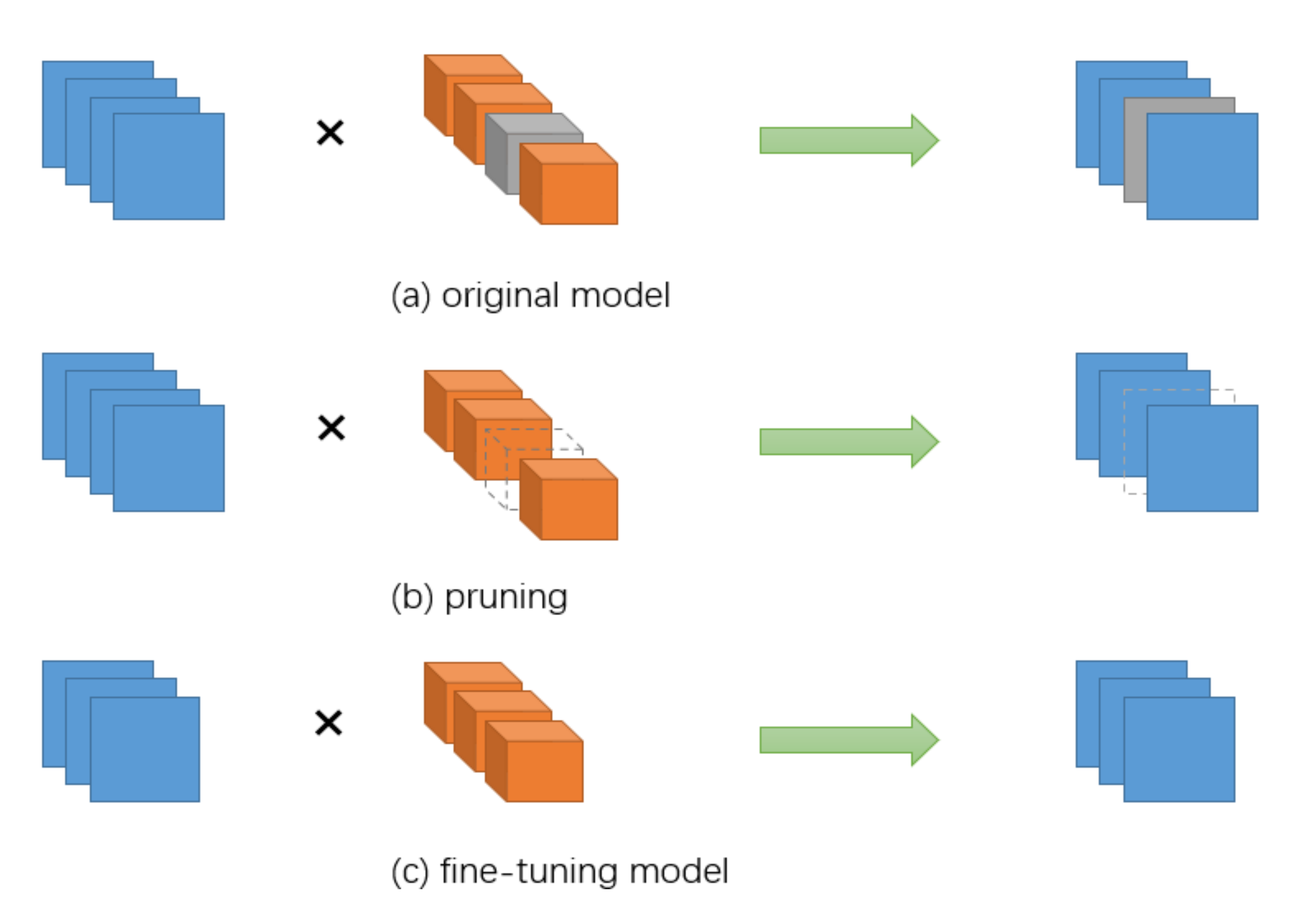
Network pruning is a widely used method in model compression. The pruning steps are generally divided into three steps: model pre-training, pruning, and parameter fine-tuning. Figure 1 shows the general network pruning process. The initial step is model pre-training, which means that the original model is trained to adjust the weight parameters, and the more important purpose of pre-training is to find out what is “important”. The second step is pruning, which generally involves determining which weights are to be removed based on the proposed decision criteria. The final step is fine-tuning, i.e., retraining the pruned network model. After pruning, there may be a loss in accuracy, and this step is used to achieve the purpose of restoring accuracy.

Figure 1.
Schematic diagram of model pruning.
2.1. Unstructured Pruning
Pruning algorithms can be classified into structured pruning and unstructured pruning based on the level of detail. In the early days, LeCun et al. [17] and Hassibi et al. [18] employed the Hessian matrix of the loss function to determine the redundant connections in the network. However, the Hessian matrix itself consumes a lot of computation time for second-order computation and takes a long time to train. Dong et al. [19] further improved the method by restricting the computation of the Hessian matrix to a single-layer network, which greatly reduced the computational effort. Han et al. [20] proposed iterative pruning, which continuously pruned and retrained the network, and obtained a simplified model after convergence, which shortened the network length compared to the method of LeCun et al. [17] training time. In addition, Guo et al. [21] improved the method of Han et al. [20]. Faced with the problem that important filters may be removed during the pruning process, resulting in a drop in accuracy, this method allows the pruned neurons to be restored again during the training process. Similarly, Zhou et al. [22] proposed to prune unimportant nodes based on the magnitude of activation values. Srinivas and Babu et al. [23] proposed a pruning framework that does not rely on training data from the perspective of the existence of redundancy among neurons, where the redundancy of nodes is calculated and removed. Chen et al. [24] proposed the HashedNets model, which introduces a hash function to group the weights according to the Hamming distance between parameters to achieve parameter sharing.
However, weight pruning is unstructured pruning, and the unstructured sparse structure is not conducive to parallel computing and requires special software or hardware for acceleration, as opposed to structured pruning, which does not have these limitations.
2.2. Structured Pruning
Structured pruning is operated on channels or entire filters without destroying the original convolutional structure, compatible with existing hardware and libraries, and more suitable for deployment on hardware. Both unstructured pruning and structured pruning require the evaluation of parameter importance. Liu et al. [25] proposed a channel-level pruning method that uses the scale factor of the BN layer as a measure to achieve compressed model size acceleration operations. Inspired by this, Kang and Han [26] considered channel scaling and shifting parameters for pruning. Yan et al. [27] combined -norm parameters and computational power as pruning criteria. SFP [28] allows the pruned filters to be updated during the training process. The convolutional kernels that were pruned in the previous training round are still involved in the iterations in the current training round, so these convolutional kernels are not directly discarded. This approach can greatly maintain the capacity of the model and obtain excellent performance. Luo et al. [29] proposed a channel pruning algorithm for ThiNet. They defined the channel pruning form as an optimization problem, using the statistics of the next layer to guide the pruning of the current layer. Redundant channels are selected based on a greedy strategy, and then the model is fine-tuning by minimizing the reconstruction error before and after pruning. Jin et al. [30] proposed structured pruning of neural networks followed by weight pruning to further compress the network model. Hu et al. [31] proposed Average Percentage Of Zeros (APOZ) to measure the number of activations to zero in each convolutional kernel as a way to evaluate the importance of convolutional kernels and perform pruning. Molchanov et al. [32] viewed the pruning problem as a combinatorial optimization problem in which an optimal subset of multiple parameters is selected to minimize the change in the model loss function after pruning. Redundant channels were selected by Taylor expansion and evaluated the effect of channel pruning on the model. Luo and Wu et al. [33] used the results of the output feature mapping GAP to obtain the information entropy and remove the redundant filters. Similarly, Yu et al. [34] optimized the reconstruction error of the final output response, and made an importance score for each channel propagation. Lin et al. [35] introduced dynamic coding filter fusion (DCFF) to train compact convolutional neural networks. Wen et al. [36] used Group Lasso for structured sparsity. Huang and Wang et al. [37] performed structured pruning by introducing learnable masks and using APG algorithm for mask sparsification.
All of the above structural pruning methods use only the parameter information of a single layer to select redundant parameters, and do not take advantage of the dynamics of network parameter updates to select redundant filters flexibly. In addition, there is noise in the parameters of the filters themselves, and these methods do not reduce the influence of interference information, which affects the correct selection of redundant filters. The fusion pruning method proposed in this paper uses the filter itself as well as information entropy stratification and BN layer parameter information to jointly select redundant parameters more accurately by combining multiple determination values.
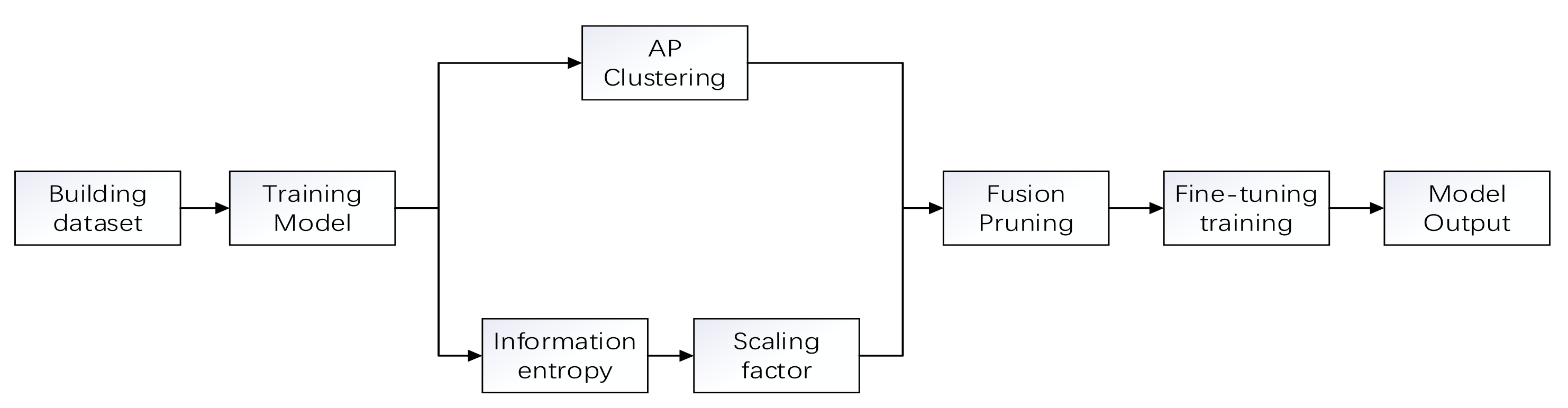
3. Fusion Pruning Algorithm
The main idea of the network pruning method is to judge the weights or convolutional kernels that are less important in the model. We remove these and then recover the model performance by the fine-tuning. It is achieved to compress the neural network model parameters to the maximum extent to achieve model acceleration while guaranteeing the model performance.
In the previous filter pruning methods, most of them were judged by the value of the -norm or -norm to determine whether they were significant or not. However, based on this method is the assumption that the minimum value satisfying the filter norm should be small enough and the variance should be large enough. Obviously, most of them do not meet this requirement. Therefore, a fusion pruning method based on information entropy hierarchy is proposed, and its process is schematically shown in Figure 2.
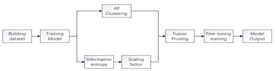
Figure 2.
Flow chart of pruning algorithm in this paper.
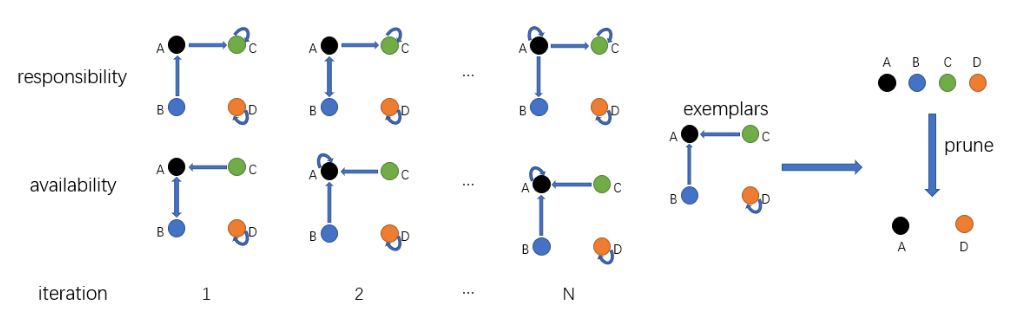
3.1. Filter Pruning Based on Affinity Propagation
Affinity Propagation (AP) was originally proposed as a paradigm for selecting data points with different attributes. All samples are considered as nodes in the network, and then the clustering center of each sample is calculated based on the message transmission of each edge in the network. There are two kinds of messages passed among the nodes during clustering, which are responsibility and availability. Affinity Propagation algorithm [38] continuously updates the responsibility and availability values of each point through an iterative process until high-quality exemplars (similar to the center of mass) are produced, while the remaining data points are assigned to the corresponding clusters.
As shown in Figure 3, it is proposed to reformat each filter as a high-dimensional data point into vector form. For any two filters, Affinity Propagation takes their similarity graph as input, which reflects the extent to which the filter is suitable as an example of the filter. The negative Euclidean distance is:
when , it expresses the adaptability of the filter to its own samples (self-similarity). It can be defined as:
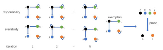
Figure 3.
Schematic diagram of clustering.
The function returns a middle value of the input.
Larger results in more example filters, however, this will reduce complexity. Using the median of the total weights of the k-th layer in Equation (2), a moderate number of samples can be obtained. To solve, Equation (2) was restated as follows:
where is a pre-given hyperparameter.
Equation (3) differs from Equation (2) in two ways: first, the median is obtained on the i-th filter, rather than the whole weight. Therefore, the similarity can be more adapted to the filter . Second, the introduced provides an adjustable model complexity reduction, with larger β reducing very high complexity and vice versa.
In addition to similarity, two other messages are passed between filters—responsibility and availability—to determine which filter is the paradigm, and which paradigm it belongs to for each other filter.
By considering other potential examples of the filter , responsibility indicates the filter and whether it is suitable as a filter paradigm of the filter. The update of the is as follows:
where is initialized to zero, which is the following “availability”. The is set to minus the maximum similarity between the filter and the other filters. Afterwards, if a filter is assigned to other samples, its availability degree is all less than zero in Equation (6), which further reduces the validity of in Equation (4) and thus will be removed from the candidate samples.
For , the “self-responsibility” is defined as follows:
It is set to minus the maximum similarity between the filter and the other filters. It reflects the possibility that the filter is an example.
As for availability, its update rule is first given as follows.
The availability is set to the sum of plus the other responsibilities of the filter. excludes the negative responsibility, since only good filters (positive responsibility) need to be focused on. indicates that the filter is better suited to belong to another paradigm rather than the paradigm itself. It can be seen that the availability of a filter as an exemplar increases if some other filter has a positive responsibility towards it. Thus, the degree of belonging reflects the suitability of the choice as its paradigm, as it takes into account the support of other filters that should be used as paradigms. Finally, limits the effect of strong positive responsibility so that the sum cannot exceed zero.
For , the “self-availability” is given as:
This reflects that the filter is an example of the positive responsibilities based on other filters.
The updates of responsibility and availability are iterative. To avoid numerical oscillations, consider the weighted sum of each message at the t-th update stage.
where is the weighting factor.
After a fixed number of iterations, the filter, as its example, satisfies.
when , the filter selects itself as an example. All the selected filters make up the examples. Therefore, the number of samples is adaptive and there is no artificial identification.
3.2. Channel Pruning Based on Batch Normalization (BN) Layer Scaling Factor
The Batch Normalization (BN) layer has been widely used in neural networks due to its role in accelerating the convergence of the network and is generally placed in the next layer of the convolutional layer to normalize the features to the output of the convolutional layer, allowing each layer of the network to learn on its own, slightly independent of the other layers. BN layer has two optimization parameters—the scaling factor and the offset factor—which fine-tune the normalized feature data so that the feature values can learn the distribution of features in each layer. The Algorithm 1 is the forward propagation process.
| Algorithm 1 Batch Normalizing Transform. |
| Input: values of x over a mini-batch: B = {}; Parameters to be learned: |
| Output. |
| //mini-batch mean |
| 2. //mini-batch variance |
| 3. //normalize |
| 4. //scale and shift |
is the mean of the input and is the variance. The convolution layer produces a feature map for each filter when the convolution operation is performed, and each feature map has a unique correspondence when normalization is performed. Thus, the feature map can be determined by the scaling factor and then the corresponding filter can be selected by the feature map, from which the importance of the filter can be determined.
3.3. Fusion Pruning
In order to achieve the most refined and simplified network model structure, the fusion pruning method combines two pruning methods, filter clustering and information entropy hierarchy, to remove the redundant filters and channels. On the one hand, the redundant filters are searched for from the filter perspective. On the other hand, based on the information entropy hierarchy, the importance between each layer is judged from the layer perspective to determine the pruning rate of each layer, and then channel pruning is performed to remove the redundant channels.
Since the importance of each layer of the convolutional layer is different, pruning with the same pruning rate may lead to pruning of important features of some layers. Therefore, a channel pruning method of the information entropy hierarchy based on the scale factor of the BN layer is proposed. Based on the range of scaling factor value sizes, this value interval is divided equally into a number of intervals, denoted as N, and counts the probability of each weight in different intervals. The entropy value can be calculated by the following equation.
where denotes the entropy value of the j-th scaling coefficient in the i-th layer, and denotes the probability that the scaling factor is in a certain interval.
J denotes the total number of features in the current layer. is the final score entropy value of the current layer, which can reflect the dispersion degree of the current layer. According to the degree of dispersion by which the layer weight fluctuation size can be known, the greater the fluctuation, the more features contained, and vice versa, the less features contained. The K-class pruning rate can be set and the entropy value can be classified using k-means. According to the classification results, they correspond to different pruning rates—a high entropy value corresponds to a low pruning rate and a low entropy value corresponds to a high pruning rate. Algorithm 2 represents the k-means clustering process.
| Algorithm 2 The K-Means Clustering. | |
| Input: sample set | |
| Number of clusters K | |
| Process: | |
| 1: | K samples are randomly selected from T as the initial mean vector: |
| 2: | repeat |
| 3: | Cause |
| 4: | for do |
| 5: | Calculate the distance between the sample and each mean vector : ; |
| 6: | Determined from the nearest mean vector of the cluster markers: ; |
| 7: | Place the samples Classify into the appropriate clusters |
| 8: | end for |
| 9: | for do |
| 10: | Calculate the new mean vector: ; |
| 11: | if then |
| 12: | Update the current mean vector to ; |
| 13: | else |
| 14: | Keep the current mean vector constant |
| 15: | end if |
| 16: | end for |
| 17: | until none of the current mean vectors are updated |
| Output: Cluster division | |
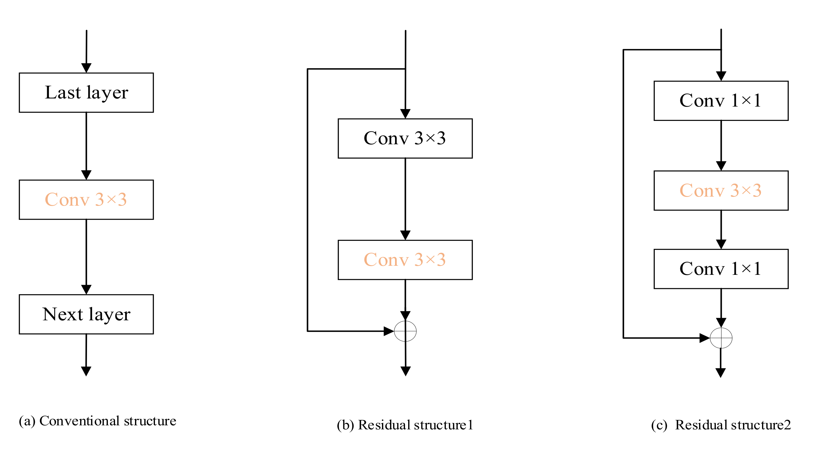
In this paper, it is pruned by the pruning method mentioned above to achieve a network model with maximum proportional compression. Figure 4 shows different pruning strategies for different network structures. Algorithm 3 describes the fusion pruning process. The fusion pruning algorithm takes the training data, the original VGG16 network, the initialized weights, and the high and low pruning rates as input and the network obtained after pruning as output.
| Algorithm 3 Fusion Pruning Algorithm. |
| 1: Trained the original VGG16 network on the training set. |
| 2: Selection of convolutional layers for prunable networks. |
| 3: Clustering of the network to obtain m categories. |
| 4: Obtain the redundant filters to be removed, based on the samples from each category. |
| 5: After step 2, calculate the entropy value using a range of scaling factor values. 6: Determine the pruning rate of each layer by dividing into N classes using k-means. 7: Ranking the scaling factors of each convolutional layer and obtaining the channels to be removed according to the pruning rate P of that layer. |
| 8: Merge the results obtained in steps four and seven. |
| 9: Remove the sum obtained in step eight after step two to obtain the streamlined network structure. |
| 10: Fine-tuning the new network on the training data to get the final model. |
Figure 4.
Different network pruning strategies.
4. Experiment
In order to verify the effectiveness of the model pruning algorithm, the experimental session of this paper will be based on the pytorch framework, based on the VGG model and the Resnet model.
The experimental equipment used in this paper is based on Windows 10 with processor Intel(R) Core (TM) i5-10300H CPU @ 2.50GHz, graphics card NVIDIA GeForce GTX 1650, in virtual environment PyCharm 2020.1.2 (Professional Edition), pytorch 1.8.0, torchversion 0.9.0, CUDA version 10.2.89.
First, experiments were conducted for pruning tests on a dataset containing 10 common objects, CIFAR-10. The CIFAR-10 dataset has a total of 60,000 images, all 32 × 32 pixels in size in color, divided into 10 categories in total. When conducting the experiments, they were generally divided into 50,000 training set images and 10,000 validation set images.
We select several existing algorithms and compare them objectively with the algorithm proposed in this paper in accuracy and parameter compression ratio to verify the advantages and disadvantages of the fusion pruning algorithm. The experimental results of different pruning algorithms are compared on the CIFAR-10 dataset based on the vgg16 model and the resnet56 model.
As shown in Table 1, we analyzed on cifar10 through VGG16 and ResNet56. More detailed analyses are provided as below:

Table 1.
Pruning result on CIFAR-10.
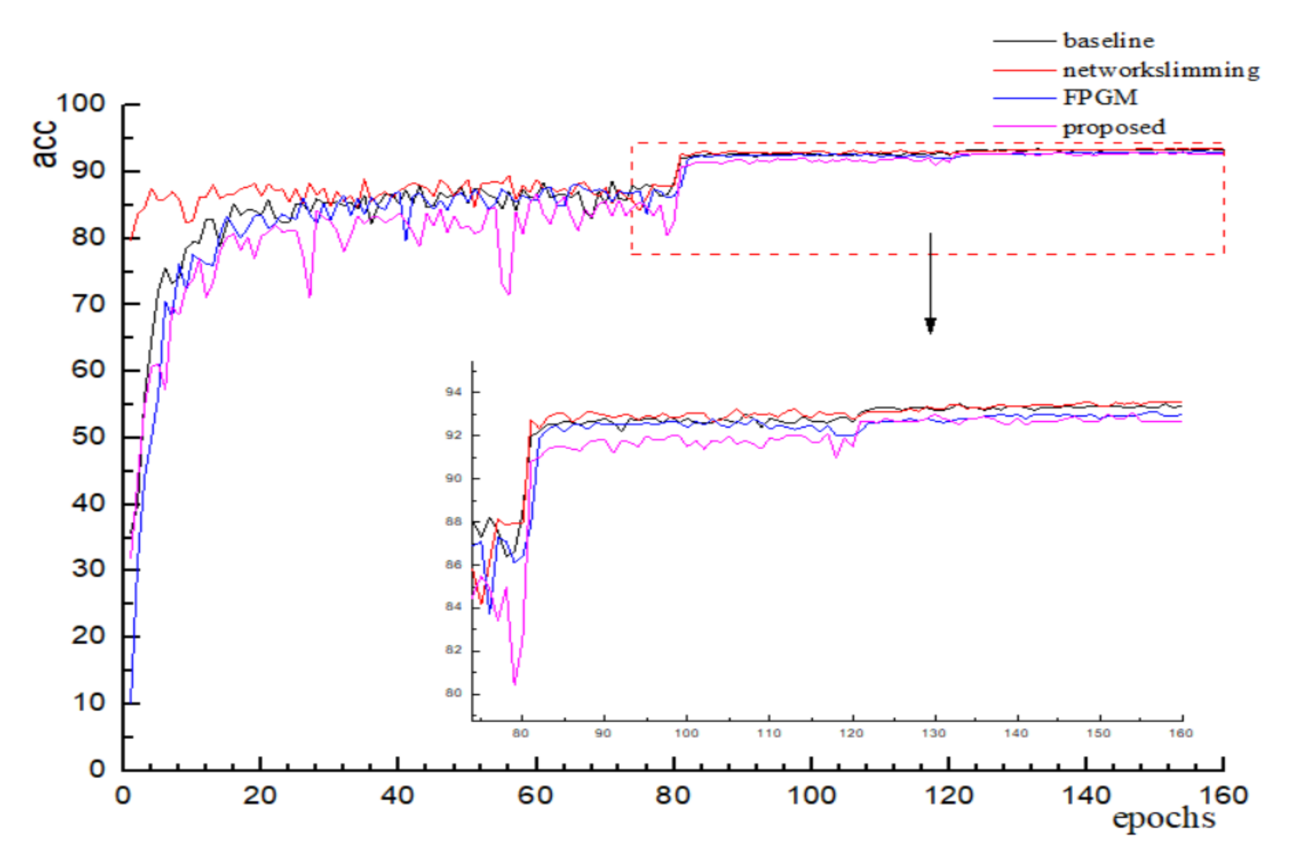
VGGNet-16. After pruning and fine-tuning, several different algorithms’ accuracy variation is shown in Figure 5 below, and it can be found that the final convergence values do not differ much. The accuracy of the proposed pruning method did not lose much accuracy compared to the other algorithms, which is in accordance with the experimental expectations. As shown in Table 1 below, it can be found that the FPGM uses a geometric center-based filter evaluation metric with a small difference in accuracy, but only 34.22% reduction in floating point computation. The literature [25] reduces half of the computation by sparsifying the scale factor evaluation and reduces the parameter volume to 1.83 M. Compared with other algorithms, the algorithm in this paper prunes from both filter and channel perspectives, which greatly compresses the number of parameters as well as the computation volume while ensuring that the pruning accuracy remains basically the same, and achieves the purpose of streamlining and accelerating the network model.
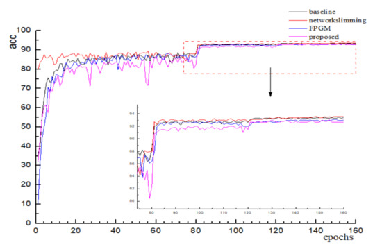
Figure 5.
Variation of accuracy in VGG16.
ResNet-56. On CIFAR10, with similar parameters and FLOPs, our algorithm based on information entropy stratification enables ResNet56 to obtain an accuracy of 93.21% with 0.31 M parameters and 45.78 M FLOPs, respectively. In addition, using our fusion pruning algorithm is effective in reducing the computation with a slight loss of accuracy. This shows that our algorithm is suitable for pruning residual blocks.
5. Case Study
5.1. Development of the Internet of Things (IoT)
Since the launching of Google’s head-mounted device, quite a lot of attention has been paid to wearable (electronic) devices. In recent years, major technology companies have also started to develop novel wearable devices. Samsung launched its first smartwatch, the Samsung Galaxy Gear, in 2013, and Apple followed a year or so later with its own smartwatch offshoot, the Apple Watch. In the field of virtual reality, HTC also announced a new generation of VR headsets in 2016, which allows users to move freely in virtual space-time. It shows that wearable devices have significant market space and have a wide range of applications, including health, entertainment, and military. For example, wearable sensing can provide responsive early warning to patients following episodes of Parkinson’s disease, heart attack, sleep apnea, and other diseases. In these sudden moments, patients are likely to lose consciousness or mobility instantly, and wearable devices can save lives. For certain body signals that are difficult to observe directly, such as pulse and sweat secretion, IoT devices can achieve timely and continuous detection, and can sustainably make health assessment to protect life. On the other hand, IoT applications are not uncommon in life. Kumar [41] proposes a public transportation system mask detection system to guarantee public transportation safety. Tarek [42] designs a tomato leaf disease identification workstation to guard the healthy growth of vegetables.
The proliferation of mobile Internet devices and various embedded devices has created a world full of rich information. Applying deep learning techniques to IoT applications can make better use of the data collected by IoT sensors such as sound, images, etc.
Deploying deep learning solutions in IoT applications typically follows the following processes: training first, then deployment. Deep learning algorithms include both training and inference components. Training is the process of extracting valid information from existing data, while inference is the procedure of using the extracted valid information to process the data to be processed. Training a large deep learning model is a high resource process. When applying deep learning techniques to an IoT environment, the training process is usually done in a server with huge computing power before the trained model is deployed in an IoT device. However, a major design requirement for IoT devices is low power consumption, which often means limited computing power as well as storage space. Therefore, we pruned the complex network before deployment. The network pruning is intended to make the model smaller and the running time faster, suitable for deployment on IOT devices or wearable devices with weak computing power.
The purpose of the research in this section is to deploy the algorithm to the embedded platform. To demonstrate the performance on IoT devices, this experiment uses a common mobile terminal as a platform for target recognition testing. The experimental environment is Android Studio 2020.3.1, simulated device Pixel 4 API 30 Android 11.0 1080*2280:440dpi, cpu x86.
5.2. NCNN Framework
Deploying algorithms to end devices requires a deep learning framework that can achieve inference acceleration on embedded platforms. NCNN is Tencent’s open source deep learning forward framework, which has no dependency on third-party libraries and is relatively small in size and is convenient to use for deployment on the embedded platform. NCNN is not only optimized for CPU acceleration on ARM platforms, but also supports GPU acceleration. NCNN provides an interface to use Vulkan, so in practice you only need to compile the GPU version of the NCNN library, and then use GPU acceleration for model inference via Vulkan, and it is very easy to use with a single line of code command to enable GPU acceleration.
The NCNN framework builds the network and the inference process as shown in Figure 6. First, the NCNN network interface is built, then the model is initialized, and the model parameter file and the model weight file are loaded. Second, the processed network input is read, and then the network extractor is created and used to perform the forward inference process to obtain the network output, where the names of the network input and output should be consistent with those in the model parameter file.
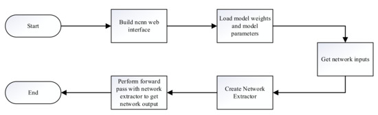
Figure 6.
The NCNN framework for building networks and the inference process.
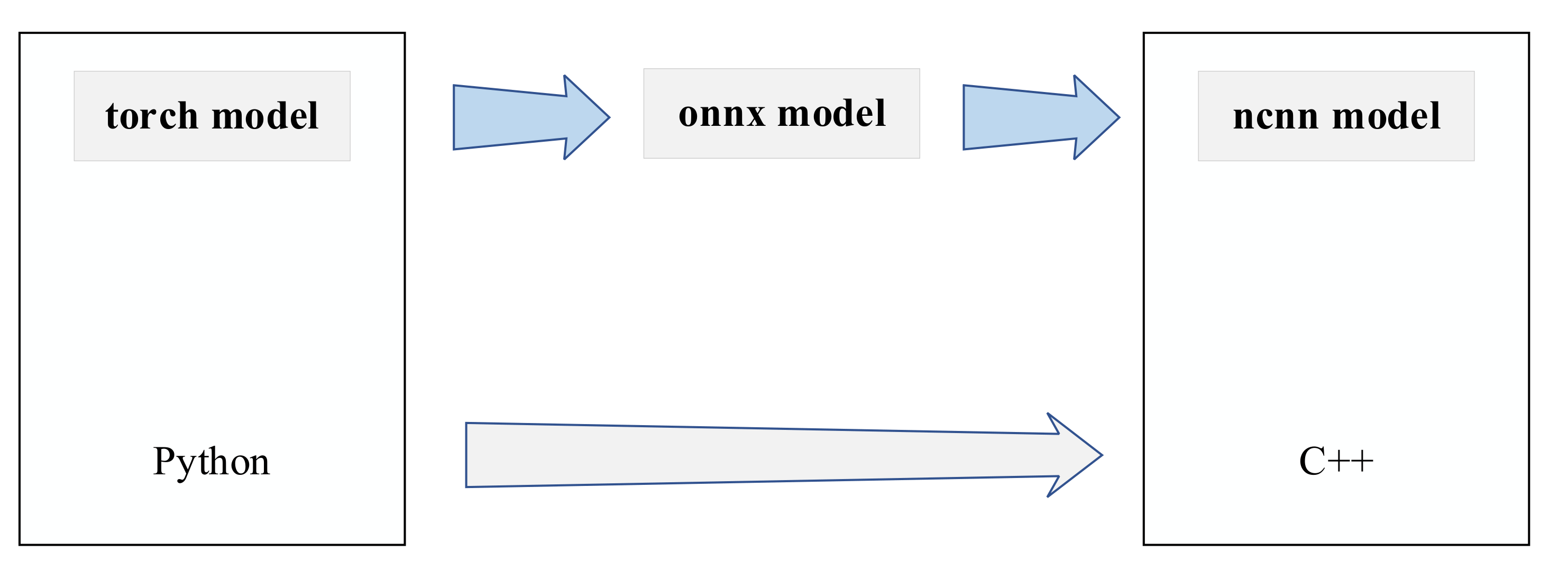
5.3. Model Conversion
The algorithm in this paper will get the model file and weight file after design and training in the Pytorch framework, but NCNN does not provide the interface to convert the Pytorch model to NCNN model directly. NCNN provides interfaces for conversion of caffe framework and onnx model formats, but the caffe framework does not provide interfaces for model conversion from Pytorch to caffe. Therefore, in this paper, we choose to convert the model from torch to the intermediate format onnx first, and then from onnx format to NCNN model, and verify the results at each conversion format. Finally, we can get the model parameter files and model weight files in NCNN format. The model conversion process is shown in Figure 7.
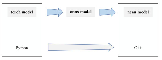
Figure 7.
Model conversion schematic.
5.4. System Construction
The flow of deploying running target recognition algorithms to identify objects based on the NCNN framework is shown in Figure 8.
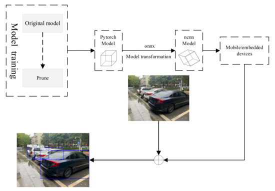
Figure 8.
System Architecture Diagram.
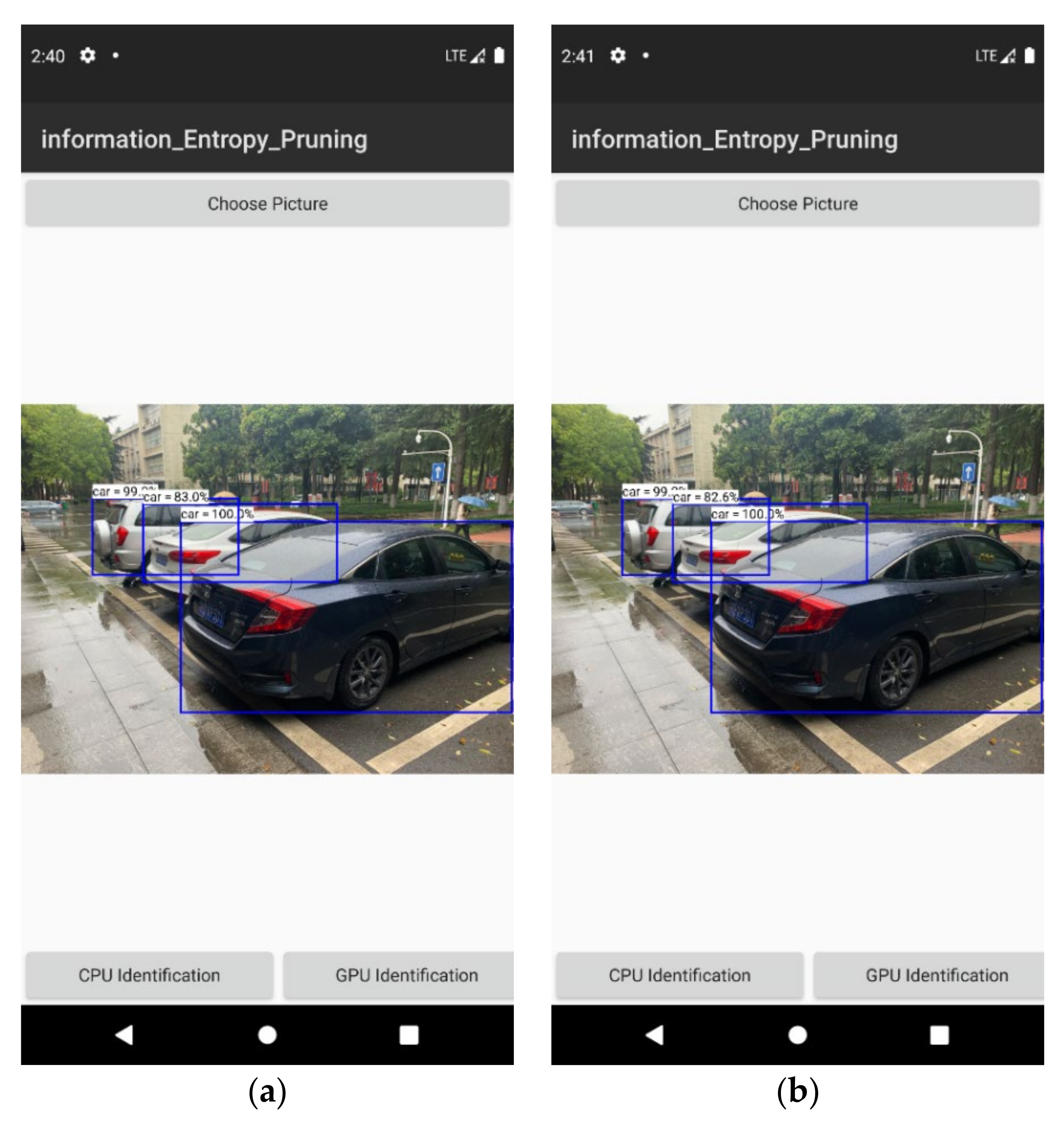
After obtaining the compressed model, we proceeded to deploy it on a mobile platform with ARM instruction set. We take VGG16 as an example to test. The over-parameterized model was implemented and trained using the Pytorch deep learning framework, which provides good computational support for X86 instruction set CPUs and Nvidia GPUs but cannot run on ARM instruction set CPUs. For this reason, we use the ONNX (Open Neural Network Exchange) specification as a transit to convert the computational graph and parameters of the model to the file format used by NCNN, and then use NCNN to perform the inference on the cell phone side. The following Figure 9 shows the running results. Table 2 compares the change in time consumption before and after pruning.
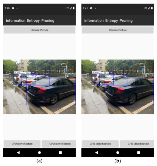
Figure 9.
Actual running results of the target recognition system. (a) is on cpu identification. (b) is on gpu identification.
Table 2.
Compute the time consumption of the model on cpu before and after pruning.
6. Conclusions
In order to obtain a more streamlined and compact network model with basically the same model accuracy, this paper proposes a fusion pruning method, which first uses filter clustering to avoid an overly concentrated weight distribution, and then prunes to remove unimportant channels according to the BN layer scaling factor based on information entropy stratification, and the two are combined to achieve maximum compression. The experimental results show that the algorithm makes the computation compressed by a factor of 4.1 and the number of parameters by a factor of 10.74 while maintaining accuracy on VGG16. There are also pretty good results on ResNet56. After the algorithm is deployed to the device for testing, it still shows excellent performance. The current experiments have proved that, compared with the original deep learning model, the algorithm proposed in this paper has great improvements in both running time and space. The optimized model deployment is only on the mobile side, not really running on wearable devices, and its performance and expansion space have not been fully verified. Our future work will be carried out in this area, and we will try to add quantification methods to further optimize the model.
Author Contributions
Investigation, M.L.; resources, S.-L.P.; supervision, M.H. and M.L.; funding acquisition, M.Z.; writing—original draft preparation, M.H. and J.T.; writing—review and editing, M.Z., M.H., M.L., S.-L.P. and J.T. All authors have read and agreed to the published version of the manuscript.
Funding
This research was funded by Hubei Provincial Department of Education: 21D031.
Conflicts of Interest
The authors declare no conflict of interest.
References
- Simonyan, K.; Zisserman, A. Very deep convolutional networks for large-scale lmage recognition. arXiv 2014, arXiv:1409.1556. [Google Scholar]
- Szegedy, C.; Liu, W.; Jia, Y.; Sermanet, P.; Rabinovich, A. Going Deeper with Convolutions. In Proceedings of the IEEE Conference on Computer Vision and Pattern Recognition, Boston, MA, USA, 7–12 June 2015. [Google Scholar] [CrossRef] [Green Version]
- He, K.; Zhang, X.; Ren, S.; Sun, J. Deep Residual Learning for Image Recognition. In Proceedings of the 2016 IEEE Conference on Computer Vision and Pattern Recognition (CVPR), Las Vegas, NV, USA, 27–30 June 2016. [Google Scholar]
- Huang, G.; Liu, Z.; Laurens, V.; Weinberger, K.Q. Densely Connected Convolutional Networks. In Proceedings of the IEEE Conference on Computer Vision and Pattern Recognition, Honolulu, HI, USA, 21–26 July 2017. [Google Scholar]
- Iandola, F.N.; Han, S.; Moskewicz, M.W.; Ashraf, K.; Dally, W.J.; Keutzer, K. SqueezeNet: AlexNet-level accuracy with 50× fewer parameters and <0.5 MB model size. arXiv 2016, arXiv:1602.07360. [Google Scholar]
- Howard, A.G.; Zhu, M.; Chen, B.; Kalenichenko, D.; Wang, W.; Weyand, T.; Andreetto, M.; Adam, H. MobileNets: Efficient Convolutional Neural Networks for Mobile Vision Applications. arXiv 2017, arXiv:1704.04861. [Google Scholar]
- Zhang, X.; Zhou, X.; Lin, M.; Sun, J. ShuffleNet: An Extremely Efficient Convolutional Neural Network for Mobile Devices. arXiv 2017, arXiv:1707.01083v2. [Google Scholar]
- He, Y.; Liu, P.; Wang, Z.; Hu, Z.; Yang, Y. Filter Pruning via Geometric Median for Deep Convolutional Neural Networks Acceleration. In Proceedings of the 2019 IEEE/CVF Conference on Computer Vision and Pattern Recognition (CVPR), Long Beach, CA, USA, 16–20 June 2019. [Google Scholar]
- Li, H.; Kadav, A.; Durdanovic, I.; Samet, H.; Graf, H.P. Pruning Filters for Efficient ConvNets. arXiv 2016, arXiv:1608.08710. [Google Scholar]
- Zhang, X.; He, Y.; Jian, S. Channel Pruning for Accelerating Very Deep Neural Networks. In Proceedings of the IEEE International Conference on Computer Vision, Venice, Italy, 22–29 October 2017. [Google Scholar]
- Zhao, M.; Li, M.; Peng, S.-L.; Li, J. A Novel Deep Learning Model Compression Algorithm. Electronics 2022, 11, 1066. [Google Scholar] [CrossRef]
- Lin, M.; Ji, R.; Wang, Y.; Zhang, Y.; Zhang, B.; Tian, Y.; Shao, L. HRank: Filter Pruning using High-Rank Feature Map. In Proceedings of the IEEE/CVF Conference on Computer Vision and Pattern Recognition, Seattle, WA, USA, 14–19 June 2020. [Google Scholar]
- Wang, W.; Fu, C.; Guo, J.; Cai, D.; He, X. COP: Customized Deep Model Compression via Regularized Correlation-Based Filter-Level Pruning. arXiv 2019, arXiv:1906.10337. [Google Scholar]
- Ghimire, D.; Kil, D.; Kim, S.-H. A Survey on Efficient Convolutional Neural Networks and Hardware Acceleration. Electronics 2022, 11, 945. [Google Scholar] [CrossRef]
- Chin, T.W.; Ding, R.; Zhang, C.; Marculescu, D. Towards Efficient Model Compression via Learned Global Ranking. arXiv 2019, arXiv:1904.12368. [Google Scholar]
- De Campos Souza, P.V.; Bambirra Torres, L.C.; Lacerda Silva, G.R.; Braga, A.d.P.; Lughofer, E. An Advanced Pruning Method in the Architecture of Extreme Learning Machines Using L1-Regularization and Bootstrapping. Electronics 2020, 9, 811. [Google Scholar] [CrossRef]
- Lecun, Y. Optimal Brain Damage. Neural Inf. Proc. Syst. 1990, 2, 598–605. [Google Scholar]
- Hassibi, B.; Stork, D.G. Second order derivatives for network pruning: Optimal brain surgeon. In Proceedings of the Advances in Neural Information Processing Systems, Denver, CO, USA, 30 November–3 December 1992. [Google Scholar]
- Dong, X.; Chen, S.; Pan, S.J. Learning to Prune Deep Neural Networks via Layer-wise Optimal Brain Surgeon. In Proceedings of the Advances in Neural Information Processing Systems, Long Beach, CA, USA, 4–9 December 2017. [Google Scholar]
- Han, S.; Pool, J.; Tran, J.; Dally, W.J. Learning both Weights and Connections for Efficient Neural Networks; MIT Press: Cambridge, MA, USA, 2015. [Google Scholar]
- Guo, Y.; Yao, A.; Chen, Y. Dynamic Network Surgery for Efficient DNNs. In Proceedings of the Nips, Barcelona, Spain, 5–10 December 2016. [Google Scholar]
- Zhou, A.Z.; Luo, K. Sparse Dropout Regularization Method for Convolutional Neural Networks. J. Chin. Comput. Syst. 2018, 39, 1674–1679. [Google Scholar]
- Srinivas, S.; Babu, R.V. Data-free parameter pruning for Deep Neural Networks. In Proceedings of the Computer Science, Swansea, UK, 7–10 September 2015; pp. 2830–2838. [Google Scholar]
- Chen, W.; Wilson, J.T.; Tyree, S.; Weinberger, K.Q.; Chen, Y. Compressing Neural Networks with the Hashing Trick. In Proceedings of the Computer Science, Swansea, UK, 7–10 September 2015; pp. 2285–2294. [Google Scholar]
- Zhuang, L.; Li, J.; Shen, Z.; Gao, H.; Zhang, C. Learning Efficient Convolutional Networks through Network Slimming. In Proceedings of the 2017 IEEE International Conference on Computer Vision (ICCV), Venice, Italy, 22–29 October 2017. [Google Scholar]
- Kang, M.; Han, B. Operation-Aware Soft Channel Pruning using Differentiable Masks. In Proceedings of the International Conference on Machine Learning, Shanghai, China, 6–8 November 2020. [Google Scholar]
- Yan, Y.; Li, C.; Guo, R.; Yang, K.; Xu, Y. Channel Pruning via Multi-Criteria based on Weight Dependency. In Proceedings of the 2021 International Joint Conference on Neural Networks, Shenzhen, China, 18–22 July 2020. [Google Scholar]
- He, Y.; Kang, G.; Dong, X.; Fu, Y.; Yang, Y. Soft Filter Pruning for Accelerating Deep Convolutional Neural Networks. arXiv 2018, arXiv:1808.06866. [Google Scholar]
- Luo, J.H.; Wu, J.; Lin, W. ThiNet: A Filter Level Pruning Method for Deep Neural Network Compression. In Proceedings of the 2017 IEEE International Conference on Computer Vision (ICCV), Venice, Italy, 22–29 October 2017. [Google Scholar]
- Yang, W.; Jin, L.; Wang, S.; Cu, Z.; Chen, X.; Chen, L. Thinning of Convolutional Neural Network with Mixed Pruning. IET Image Processing 2019, 13, 779–784. [Google Scholar] [CrossRef]
- Hu, H.; Peng, R.; Tai, Y.W.; Tang, C.K. Network Trimming: A Data-Driven Neuron Pruning Approach towards Efficient Deep Architectures. arXiv 2016, arXiv:1607.03250. [Google Scholar]
- Molchanov, P.; Tyree, S.; Karras, T.; Aila, T.; Kautz, J. Pruning Convolutional Neural Networks for Resource Efficient Transfer Learning. arXiv 2016, arXiv:1611.06440. [Google Scholar]
- Luo, J.H.; Wu, J. An Entropy-based Pruning Method for CNN Compression. arXiv 2017, arXiv:1706.05791. [Google Scholar]
- Yu, R.; Li, A.; Chen, C.F.; Lai, J.H.; Davis, L.S. NISP: Pruning Networks Using Neuron Importance Score Propagation. In Proceedings of the IEEE/CVF Conference on Computer Vision & Pattern Recognition, Salt Lake City, UT, USA, 18–22 June 2018. [Google Scholar]
- Lin, M.; Ji, R.; Chen, B.; Chao, F.; Liu, J.; Zeng, W.; Tian, Y.; Tian, Q. Training Compact CNNs for Image Classification using Dynamic-coded Filter Fusion. arXiv 2021, arXiv:2107.06916. [Google Scholar]
- Wen, W.; Wu, C.; Wang, Y.; Chen, Y.; Li, H. Learning Structured Sparsity in Deep Neural Networks. In Proceedings of the Advances in Neural Information Processing Systems, Barcelona, Spain, 5–10 December 2016. [Google Scholar]
- Huang, Z.; Wang, N. Data-Driven Sparse Structure Selection for Deep Neural Networks. In Proceedings of the European Conference on Computer Vision (ECCV), Venice, Italy, 22–29 October 2017. [Google Scholar]
- Lin, M.; Ji, R.; Li, S.; Wang, Y.; Ye, Q. Network Pruning Using Adaptive Exemplar Filters. IEEE Trans. Neural Netw. Learn. Syst. 2021. [Google Scholar] [CrossRef]
- Lin, M.; Ji, R.; Li, S.; Ye, Q.; Tian, Y.; Liu, J.; Tian, Q. Filter Sketch for Network Pruning. arXiv 2020, arXiv:2001.08514. [Google Scholar] [CrossRef]
- Li, Y.; Lin, S.; Zhang, B.; Liu, J.; Ji, R. Exploiting Kernel Sparsity and Entropy for Interpretable CNN Compression. In Proceedings of the 2019 IEEE/CVF Conference on Computer Vision and Pattern Recognition (CVPR), Long Beach, CA, USA, 15–20 June 2019. [Google Scholar]
- Kumar, T.A.; Rajmohan, R.; Pavithra, M.; Ajagbe, S.A.; Hodhod, R.; Gaber, T. Automatic Face Mask Detection System in Public Transportation in Smart Cities Using IoT and Deep Learning. Electronics 2022, 11, 904. [Google Scholar] [CrossRef]
- Tarek, H.; Aly, H.; Eisa, S.; Abul-Soud, M. Optimized Deep Learning Algorithms for Tomato Leaf Disease Detection with Hardware Deployment. Electronics 2022, 11, 140. [Google Scholar] [CrossRef]


Publisher’s Note: MDPI stays neutral with regard to jurisdictional claims in published maps and institutional affiliations. |
© 2022 by the authors. Licensee MDPI, Basel, Switzerland. This article is an open access article distributed under the terms and conditions of the Creative Commons Attribution (CC BY) license (https://creativecommons.org/licenses/by/4.0/).