A Graph Attention Mechanism-Based Multiagent Reinforcement-Learning Method for Task Scheduling in Edge Computing

Abstract

Multi-access edge computing (MEC) enables end devices with limited computing power to provide effective solutions while dealing with tasks that are computationally challenging. When each end device in an MEC scenario generates multiple tasks, how to reasonably and effectively schedule these tasks is a large-scale discrete action space problem. In addition, how to exploit the objectively existing spatial structure relationships in the given scenario is also an important factor to be considered in task-scheduling algorithms. In this work, we consider indivisible, time-sensitive tasks under this scenario and formalize the task-scheduling problem to minimize the long-term losses. We propose a multiagent collaborative deep reinforcement learning (DRL)-based distributed scheduling algorithm based on graph attention neural networks (GATs) to solve task-scheduling problems in the MEC scenario. Each end device creates a graph representation agent to extract potential spatial features in the scenario and a scheduling agent to extract the timing-related features of the tasks and make scheduling decisions using a gated recurrent unit (GRU). The simulation results show that, compared with several baseline algorithms, our proposed algorithm can take advantage of the spatial positional relationship of devices in the environment, significantly reduce the average delay and drop rate, and improve link utilization.

1. Introduction

Currently, with the booming development of short-range communication technologies, network transmission efficiency and bandwidth levels are significantly improving, making short-range wireless data transmission increasingly convenient and fast. Multi-access edge computing (MEC) [1] is considered an effective solution for handling computationally intensive tasks because of its low latency and high computational performance [2].

Although MEC has advantages over cloud computing in multiple scenarios, typical edge-layer stations are limited in terms of computational power as they consist of smart wireless base stations, which also have limited computational power [3,4]. In addition, task arrival uncertainty in the network state poses significant challenges for task scheduling. For example, if a large number of terminal devices in an MEC scenario randomly schedule tasks to the edge nodes, this may lead to unbalanced edge node loads [5]. Thus, because the dropout rates of tasks increase after the processing deadline is exceeded, an inappropriate MEC task scheduling algorithm cannot meet the task deadline requirements to a certain extent.

When facing this type of multiobjective optimization problem, it is difficult for traditional optimization techniques to obtain strong results [6,7]. Therefore, in an MEC system, selecting the appropriate edge server for global task scheduling is a PSPACE-hard problem [8], which is more difficult to solve in polynomial time than a nondeterministic polynomial (NP)-hard problem. Reinforcement learning is considered the quintessential MEC task scheduling solution due to its powerful learning capabilities. The use of deep reinforcement learning (DRL) to optimize the task scheduling process in MEC has become a new research trend [9,10,11,12,13,14]. In many distributed scheduling algorithms that use reinforcement learning to solve task scheduling problems, each end node trains a reinforcement learning agent, and each agent needs to make task scheduling decisions for the generated tasks; such approaches have achieved good results.

However, on the one hand, many existing studies model only the nodes themselves and do not consider global information, such as the potential spatial relationships in the MEC scenario and the connectivity between nodes. On the other hand, existing work assumes a “single-task problem”, where each node generates one task at the beginning of each time interval, but, in real life, end devices often generate multiple tasks at the beginning of each time slice. Assuming that each end node has L tasks arriving simultaneously and that edge-layer nodes have N optional nodes for scheduling, the action space is then $N+1$ to the Lth power. Existing reinforcement-learning-based distributed scheduling algorithms utilizing value-based deep Q-learning networks (DQNs) and policy-based actor–critic (AC) architecture algorithms do not handle large-scale discrete action spaces effectively [15], it is difficult for them to effectively and reasonably schedule multiple tasks generated at the same time, and they cannot meet the time-sensitive requirements of tasks.

In this work, we focus on the task offloading problem in MEC systems and propose a distributed algorithm to carry out the task-scheduling problem for end devices, which can make good use of the potential spatial correlation features in the scenario, and can effectively schedule multiple tasks. Considering the selfish behavior of mobile device users, end devices can offload tasks to edge nodes that are connected to them or by forwarding tasks to other edge nodes for processing via directly connected edge nodes. Thus, our proposed scenario has multiple end nodes connected to a node in the edge layer (e.g., a 5G base station), and the individual edge nodes in the edge layer are also connected to each other via high-speed links.

To exploit the potentially available and useful spatial information in the given scenario, we utilize a graph attention network (GAT) [16] to formalize this problem. A GAT, which can efficiently perform high-level feature representation by extracting the potential spatial correlations contained in the input data, helps the algorithm learn the spatial features in the given scenario. Considering that the link features between nodes are equally important for task-scheduling decisions in MEC scenarios, we incorporate edge features by changing the GAT structure to build a graph representation agent for each node. In addition, we build a scheduling agent on each end device, and each scheduling agent contains a gated recurrent unit (GRU) [17] module and multiple decision modules to make decisions for various tasks in parallel. Ultimately, each end device collaborates with both the graph representation agent and the scheduling agent to make scheduling decisions for tasks. On the one hand, our proposed algorithm can make use of the potentially useful spatial information contained in MEC scenarios to help the end devices make task decisions, and, on the other hand, the multiple decision modules in the scheduling agent can achieve a better performance when faced with a multitask-scheduling problem. The main contributions of this work are shown below.

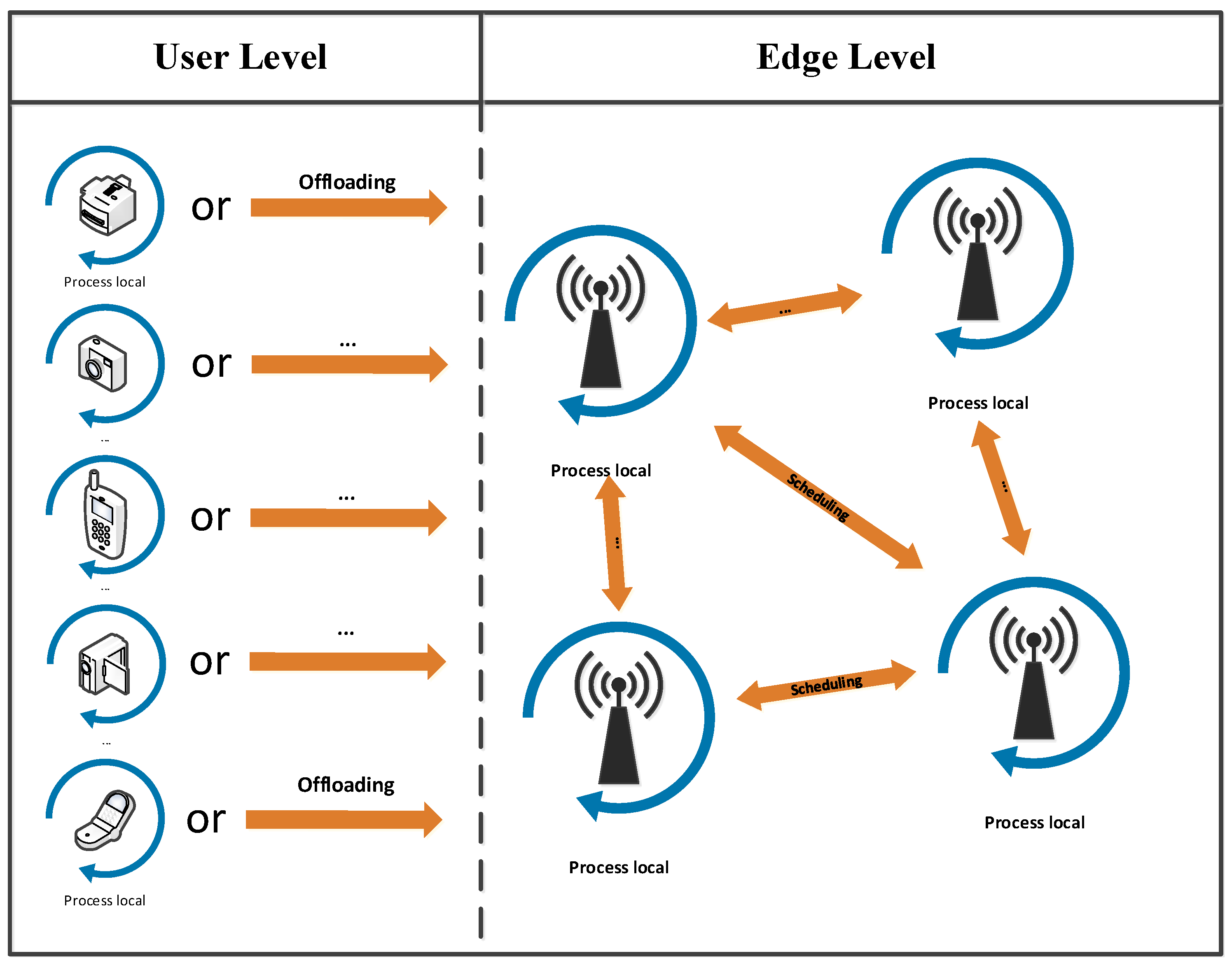
• Multitask-offloading problems in MEC scenarios
  We formally present the problem of delayed indivisible task offloading in MEC, and then we study and formulate the collaborative computing scheduling problem in terms of both processing time and bandwidth utilization. The main objectives are to minimize the long-term consumption of tasks (dropout rate due to latency and timeouts) and to efficiently schedule tasks according to latency requirements. In our considerations, the MEC distributed scheduling algorithm should consider not only the state information of individual nodes but also the interrelationships that exist between the individual nodes from a global perspective. In addition, the devices in this scenario can generate multiple tasks rather than a single-task problem.
• DRL-based offloading algorithm based on an edge GAT (E-GAT)
  Two reinforcement learning agents, the graph representation agent and the scheduling agent, are constructed in our proposed multiagent distributed scheduling algorithm with a GAT, and the task scheduling decisions are collaboratively optimized by the two agents. On the one hand, the proposed algorithm can effectively make good use of the potential spatial features contained in the scenario; on the other hand, the algorithm can make effective task-scheduling decisions by learning historical information.
• Dealing with large-scale discrete action spaces
  An analysis of the results of simulation experiments validates that our proposed algorithm has a better performance in dealing with large-scale discrete action space problem scenarios than algorithms such as the Wolpertinger architecture proposed by Google [15], and exhibits better generalization in terms of dealing with single-task scenarios.

The rest of the paper is organized as follows. Section 2 describes the background and some relevant work. Section 3 presents the system model and problem formulation. We propose a cooperative mechanism of two kind of agents, in Section 4. The task-scheduling algorithm for MEC is introduced in Section 5. We evaluate the performance of the GAT through simulations in Section 6 and demonstrate its superiority. In Section 7, we discuss the limitations of the algorithm proposed in this paper. Finally, Section 8 gives concluding remarks with possible extensions and directions for future research.

2. Related Work

In MEC, the main challenge is how to effectively perform task scheduling and offloading, and mainstream edge computing problem solving can be performed by traditional algorithms (similar to game theory) [18] and neural-network-based reinforcement learning [19] algorithms (for task-scheduling decisions).

Many methods transform the edge calculation problem into an optimization problem and then use convex optimization and other optimization methods to solve this problem. Wang et al. in [20] proposed an algorithm to determine offloading decisions by formulating them as convex optimization problems to maximize the gain. In practice, the processing capacities of edge nodes may be limited, and when a large number of mobile devices offload their tasks to the same edge node, these offloaded tasks may experience large processing delays. Some tasks may even be abandoned when the deadline expires. Wang et al. [21] considered the offloading rate, transmission power, and CPU frequency parameters to minimize the computational latency. Some works have studied the workflow scheduling problem of minimizing the maximum completion time among complex networks in a social group in an edge-computing environment. Sun et al. [22] formulated the scheduling problem as an integer-programming problem and used a greedy search strategy and a composite heuristic algorithm to guarantee the quality of the solution. Meng et al. [23] considered the scheduling problem as a date-aware task and proposed a greedy scheduling algorithm to satisfy the new deadline date. Han et al. [24] proposed a scheduling algorithm to minimize the total weighted response time across all jobs. Bi et al. in [25] considered the wireless powered MEC scenario and proposed a joint optimization method based on the alternating direction method of multipliers (ADMM) decomposition technique. Some existing works consider the load level of edge nodes and propose a centralized task-offloading algorithm. Poularakis et al. in [26] proposed an algorithm that takes the uncertainty of mobile device computational requirements into account; the algorithm minimizes the average cost and the weighted sum of cost variations. Some works have expressed the task-unloading problem as an NP-hard mixed-integer nonlinear programming problem. In [10], Chen et al. studied the offloading problem in ultra-dense networks to minimize the delay by transforming this NP-hard problem into two subproblems. Joilo, S et al. designed a distributed algorithm based on the Stackelberg game in [27]. The above scheduling algorithm using the traditional method considers delay-sensitive tasks, whereas some works consider the delay-tolerant task. Neto et al. in [28] proposed an estimation-based approach to efficiently perform task offloading and significantly reduce the energy consumption of mobile devices. In [29], Lee et al. focused on the fog network formation and task distribution problem and proposed an algorithm based on online optimization techniques to minimize the maximum latency of tasks. In addition, some works consider the load level of edge nodes and propose a distributed task-offloading algorithm. Each end device can make scheduling decisions for its own tasks. However, the distributed task-offloading algorithm will make the load level of edge layer devices unbalanced to a certain extent. To meet these challenges. Yang et al. in [30] proposed a distributed offloading algorithm to jointly optimize the energy consumption and latency of each mobile end device.

Task scheduling in MEC is a multi-objective planning problem, and the use of DRL to optimize task scheduling in MEC has become a new research trend. Some works take both the communication and computation cost into account, such as the proposed DRL-based task-scheduling algorithm. Zhan et al. [14] formulated the offloading problem as a partially observable Markov decision process (POMDP), which was solved by a policy gradient-based DRL approach. In [31], Xu et al. proposed a joint computational offloading and data-caching algorithm to reduce the overall computational latency. Yan et al. [32] developed a DRL framework to jointly optimize offloading decisions and resource allocation with the goal of minimizing the weighted sum of mobile device energy consumption and task execution time. Additionally, the wireless channel condition of the network links is a non-negligible issue in the edge-computing scenario. Huang et al. [33] proposed a DRL-based online offloading algorithm to maximize the weighted sum computation rates in wireless MEC networks with binary computation offloading. In addition, how to make good use of the historical timing information contained in edge-computing scenarios can also effectively improve the long-term payoff of the offloading decision of the algorithm in the future. Tang et al. in [34] proposed an algorithm to minimize the task-processing time by using the historical load information of the network edge layer.

Although many works have achieved good results in specific scenarios, on the one hand, the terminal device generates multiple tasks, and the scheduling problem for tasks is a large-scale discrete action space problem. On the other hand, the above works do not consider exploiting the correlation information implied by the spatial location of devices in the environment to help make task-scheduling decisions. In this work, we build a graph attention network agent to extract and learn spatial information. In addition, we build multiple parallel scheduling modules on the scheduling agent to make synchronous decisions for multiple tasks. It solves the large-scale discrete action space problem existing in the scenario.

3. System Model and Problem Formulation

The experimental simulation scenario we use in this paper is based on the scenario proposed in [34], and establishes a connection relationship between edge layer devices. Figure 1 gives an example of computation scheduling in MEC. The end device in the scenario generates multiple tasks, and this end device decides whether to schedule each task based on its information. We abstract the MEC scenario as $G=(V,E)$ with $V=\left\{M\cup N\right\}$, where E denotes the physical linkages between nodes. The path between each edge device node is calculated by a traditional shortest path algorithm, such as the Dijkstra algorithm. At the beginning of each time point t, the task to be scheduled by the end device is first transmitted to the device directly connected to it through the wireless channel according to the transmission rate $r_m$, and then the device determines whether it needs to continue the forwarding procedure. Each end device in the scenario has the same computing power $f_m^{end}$ and the same number of processing cores C. Each processing core maintains two first-in first-out ($FIFO$) processing queues. Let ${\rho }_m$ indicate the processing density of the processing tasks. As in some other works [35,36], we consider distributing the end-device-computing resources equally to each $FIFO$-processing queue. The tasks, whether they are computed locally or require scheduling, first go through these processing queues. Figure 2 is a flow chart of processing tasks generated by a end device in this scenario.

In general, task scheduling is divided into three steps. First, in each time slice t, the end device m makes scheduling decisions for tasks based on known information about the task $k_m\left(t\right)$, the link state $Link\left(t\right)$ in the scenario, the device information $U\left(t\right)$ of all devices in the MEC scenario, and the historical load information of the edge nodes $H\left(t\right)$, and places the tasks into the processing queue of the end device m. If the examined task needs to be scheduled, then the scheduling identifier $x_m\left(t\right)$ for each task is set to 1 and vice versa, and the scheduling target $y_m\left(t\right)$ is set to the corresponding edge node identifier. The end device calculates the number of time slices $\phi$ that each task must wait for processing when each task is placed in the processing queue. The task to be transmitted is sent to the edge node directly connected to it according to the transmission rate $r_n$ through the wireless link after it is processed in the queue in the end device. Second, after receiving the transmitted task, the edge-layer node first determines whether further forwarding is required based on $y_m\left(t\right)$. If forwarding is required, then this task is placed into the transmission queue for further transmission via the link. Eventually, when the task is transmitted to the final scheduling destination edge node, it is placed directly into the processing queue.

After the processing step is completed, the device calculates the time required from the beginning to the end of each task as the process delay of each task. The queues maintained by the edge nodes are called active queues if tasks are present in the queues. The number of active queues for edge node n is denoted by $Q_n\left(t\right)$, and the sum of the task bits of other devices o that are present on edge node n is defined as $g_{o,n}^{edge}\left(t\right)$. Similar to that of the end device, the computational capacity $f_n^{edge}$ of edge node n is equally distributed to each active queue, and each active queue is allocated computational resources $f_n^{edge}/Q_n\left(t\right)$. If the task is computed locally at the end device, then the task is computed directly in the processing queue of the end device, and tasks $k_m\left(t\right)$ finishes in time slice $P_m\left(t\right)$. In addition, the task is dropped when it exceeds the deadline ${\tau }_m\left(t\right)$.

3.1. Mobile Device Node

The load generated by devices tends to follow certain rules (e.g., Poisson inter-arrival time distribution [37]). At the beginning of each time slice, the end device possesses multiple tasks $k_m\left(t\right)$ and the data size of $k_m\left(t\right)$ obeys the uniform distribution. Then, this data size is multiplied by a randomly sampled value between 0 and 1 that is no larger than the task arrival probability. The size range of task size ${\lambda }_m^i\left(t\right)$ and the task arrival probability in the environment are shown in

Table 1. Parameter Settings.

Parameter	Value
$f_m^{device},m\in M$	2.5 GHz [28]
$f_n^{edge},n\in N$	41.8 GHz [28]
Mobile end device core C	4
${\lambda }_m^i\left(t\right),m\in M,i\in I,t\in T$	3.0, 3.1, ..., 10.0 Mbits [20]
$r_m\mathsf{\Delta },m\in M$	14 Mbits [34]
$r_n\mathsf{\Delta },n\in N$	41.8 Mbits
${\rho }_m,m\in M$	0.297 gigacycles per Mbits [20]
${\rho }_n,n\in N$	0.297 gigacycles per Mbits [20]
${\tau }_m^i,m\in M,i\in I$	100 time slots (10 s)
Task arrival probability	0.3

.

Each task $k_m^i\left(t\right)$ has its own information, such as its task size ${\lambda }_m^i\left(t\right)$ and task number. The tasks first enter the processing queue of the end device. Then, the end device calculates the waiting time slice ${\phi }_m^i\left(t\right)$ at which task $k_m^i\left(t\right)$ is either processed locally to completion or is dropped based on the information currently contained in the queue and the scheduling decision $x_m^i$ for task $k_m^i$. Note that the completion of the processing step mentioned here includes both computation completion and transmission completion.

$${\phi }_m^i\left(t\right)=\left[\underset{t^{\prime }\in \left\{0,1,\dots ,t-1\right\}}{max}{P}_{m,i}^c\left(t^{\prime }\right)-t+1\right]$$

(1)

$P_{m,i}^c\left(t^{\prime }\right)$ indicates the completion time of task $k_m^i\left(t^{\prime }\right)$. Since the end device observes the situation in the computing queue, including the number of tasks in the queue and the size of each task, we can calculate $P_{m,i}^c\left(t^{\prime }\right),c\in 2\ast C$ in advance when it is placed in the computing queue x.

$$P_{m,i}^c\left(t\right)=min\{t+{\phi }_m^i\left(t\right)+\left|x_m^i\left(t\right)-1\right|⌈\frac{{\lambda }_m^i\left(t\right)}{f_m^{end}\mathsf{\Delta }/{\rho }_m}⌉+x_m^i\left(t\right)\ast ⌈\frac{{\lambda }_m^i\left(t\right)}{r_m\mathsf{\Delta }}⌉-1,t+{\tau }_m^i-1\}$$

(2)

For computational convenience, let $P_{m,i}^x\left(0\right)=0$, where $⌈\ast ⌉$ represents the ceiling function. If task $k_m^i\left(t\right)$ is computed within the maximum drop time, then the time required for task computation is $⌈\frac{{\lambda }_m^i\left(t\right)}{f_m^{end}/{\rho }_m}⌉$; similarly, if it is transferred, the time required for the transfer is $⌈\frac{{\lambda }_m^i\left(t\right)}{r_m\mathsf{\Delta }}⌉$. Due to the fact that each queue contains both transfer and computation tasks, $x_m^i\left(t\right)\ast ⌈\frac{{\lambda }_m^i\left(t\right)}{r_m\mathsf{\Delta }}⌉$ represents the time required for task transfer, and $\left|x_m^i\left(t\right)-1\right|⌈\frac{{\lambda }_m^i\left(t\right)}{f_m^{end}\mathsf{\Delta }/{\rho }_m}⌉$ represents the time required for local computation. The first item of the formula is the end time of the task when completed within the specified time, the second item is the timeout time, and we take the smaller of the two items as the end time of the task execution process.

For tasks that need to be scheduled, after the end device completes transmission, each task enters the preprocessing queue of the edge node directly connected to it, and the edge node determines whether to process or forward the task based on its final scheduling destination edge node index.

3.2. Edge Server

The device possesses $3\ast N_i$ queues (each edge node maintains a preprocessing queue, a computation queue, and a transmission queue for each node directly connected to it) on each edge node $E_i$ in the edge layer, and $N_i$ represents the number of nodes (including the end device and other edge nodes) directly connected to $E_i$. At the beginning of each time slice, each edge node takes a task out of the preprocessing queue and then determines whether to process or forward it based on the associated task information; therefore, the task is placed into the corresponding computation queue or transmission queue. Note that it takes no time to transfer a task from the preprocessing queue to the computation queue or transmission queue. In time slice t, if a task $k_o^i\left(t^{\prime }\right)$ arrives at an edge node $n\in N$, we define $k_{o,n}^{edge}\left(t\right)$ = $k_o^i\left(t^{\prime }\right)$. Let ${\lambda }_{o,n}^{edge}\left(t\right)$ denote the size of the tasks from other nodes $o\in \left\{N,M\right\}$ to edge node n at the beginning of time slice t. We define $y_{o,n}^{edge}\left(t\right)=y_o^i\left(t^{\prime }\right)$ as the node to which the task is finally scheduled, and the edge node also obtains the maximum dropout time of the task assignment: ${\tau }_{o,n}^{edge}\left(t^{\prime }\right)={\tau }_o^i\left(t\right)$:

$$Q_n\left(t\right)=\sum _{i=0}^{Ni}If({\lambda }_{o,n}^{edge}\left(t\right)>0\mathrm{or}{g}_{o,n}^{edge}\left(t\right)>0)$$

(3)

The tasks in the edge layer are dropped if they are not completed by the deadline; then, we define $dro{p}_{o,n}^{edge}\left(t\right)$ as representing the total size of the tasks dropped by edge node n at the end of time slice $⌈\frac{f_n^{edge}\mathsf{\Delta }}{{\rho }_o^i{Q}_n\left(t\right)}⌉$, which represents the amount of time the task needs to be processed; similarly, $⌈\frac{{\lambda }_{o,n}^{edge}\left(t\right)}{r_n\mathsf{\Delta }}⌉$ represents the time required for task transmission to complete. Let $g{c}_{o,n}\left(t\right)$ represent the size of the processed data bits of node o on node n in time slice t.

Therefore, we can calculate $g_{o,n}^{edge}\left(t\right)$ as the size of the existing tasks in the queue of another device o on edge n according to the following steps:

$$g{c}_{o.n}^{}\left(t\right)=flag\ast ⌈\frac{f_n^{edge}\mathsf{\Delta }}{{\rho }_o^i{Q}_n\left(t\right)}⌉+flag\ast ⌈\frac{{\lambda }_{o,n}^{edge}\left(t\right)}{r_n\mathsf{\Delta }}⌉$$

(4)

$$g_{o,n}^{}\left(t\right)=\left\{g_{o,n}^{}(t-1)+{\lambda }_{o,n}^{edge}\left(t\right)-g{c}_{o,n}\left(t\right)-dro{p}_{o.n}^{edge}\left(t\right)\right\}$$

(5)

The $flag=IF(n=y_{o.n}^{edge}\left(t\right))$ in the above formula indicates whether the current node is the final scheduling destination of the task.

3.2.1. Computation Queue

At the beginning of each time slice, each edge node takes tasks from the $FIFO$ processing queue. These tasks may be transmitted directly from the end device or forwarded from another edge node. As for a mobile device node, we define $P_{o,n}^{comp}\left(t\right)$ as the time slice during which the task computation step is completed in the edge node and define ${\phi }_{o,n}^{comp}\left(t\right)$ as the time that the task must wait in the edge node from queuing to starting the computation process; this time is calculated with the following equation:

$${\phi }_{o,n}^{comp}\left(t\right)=\left[\underset{t^{\prime }\in \left\{0,1,\dots ,t-1\right\}}{max}{P}_{o,n}^{comp}\left(t\right)-t^{\prime }+1\right]$$

(6)

Similarly, for ease of calculation, we let $P_{o,n}^{comp}\left(0\right)=0$, so the final completion time of processing for the task is calculated by:

$$P_{o,n}^{comp}\left(t\right)=min\{t^{\prime }+{\phi }_{o.n}^{comp}\left(t\right)+⌈\frac{{\lambda }_{o.n}^{comp}\left(t\right)}{f_n^{edge}\mathsf{\Delta }/{\rho }_n}⌉-1,t^{\prime }+{\tau }_{o,n}^{edge}-1\}$$

(7)

The first term in the formula represents the task end time point calculated by the completion of the task before the maximum deadline, and the second term represents that the task is not completed within the maximum deadline. Then, the final processing time of the task is the maximum deadline, and the task is discarded.

3.2.2. Transmission Queue

As with the processing queue, tasks are taken out of the transmission queue at the beginning of each time slice and forwarded according to a predefined shortest path algorithm. We similarly define $P_{o,n}^{tran}\left(t\right)$ as the time slice in which the task completes its computation in the edge node and define ${\phi }_{o,n}^{tran}\left(t\right)$ as the time that the task must wait from queuing to the start of the computation process in the edge node. ${\phi }_{o,n}^{tran}\left(t\right)$ is computed in the same way as in the computation queue, which is as follows:

$${\phi }_{o,n}^{comp}\left(t\right)=\left[\underset{t^{\prime }\in \left\{0,1,\dots ,t-1\right\}}{max}{P}_{o,n}^{tran}\left(t\right)-t^{\prime }+1\right]$$

(8)

The transmission completion time $P_{o,n}^{tran}\left(t\right)$ of task $k_{o,n}^{edge}\left(t\right)$ is calculated by:

$$P_{o,n}^{tran}\left(t\right)=min\{t^{\prime }+{\phi }_{o.n}^{tram}\left(t\right)+⌈\frac{{\lambda }_{o.n}^{comp}\left(t\right)}{r_n\mathsf{\Delta }}⌉-1,t^{\prime }+{\tau }_{o,n}^{edge}-1\}$$

(9)

The first term of the formula represents the time node for completing the task within the maximum deadline for transmission, and the second term represents that the task is not completed within the maximum deadline. Then, the final processing time of the task is the maximum deadline, and the task is dropped.

3.3. Problem Formulation in the Multitask MEC Scenario

At the beginning of each time interval, the terminal device generate multiples time-sensitive tasks according to a certain probability. The terminal device makes scheduling decisions about the tasks by observing the relevant information in the scenario as well as the known information about the tasks; the ultimate goal is to minimize the average delay of the tasks generated by the device and the discard rate due to timeouts. The end device solves this multiobjective scheduling problem by using reinforcement learning; essentially, by constructing a reasonable mapping relationship from $state$ to $action$, which, in turn, can minimize the long-term expense $Cos{t}_m$ of device m:

$${\pi }_m=argminimize\mathrm{E}\left[\sum _{\mathrm{t}\in \mathrm{T}}^{}{\gamma }^{\mathrm{t}-1}\mathrm{Cos}{t}_m^{}|{\pi }_m\right]$$

(10)

${\pi }_m$ is the parameter of the mapping relationship, the formula $\mathrm{E}$ represents mathematical expectation, and $\gamma$ represents the decay factor.

4. Multiagent Cooperation

In this section, we introduce the graph representation agent for extracting spatial feature information, the scheduling agent for making decisions by using spatial and temporal information, and the message passing logic between them.

4.1. Graph Representation Agent

A $\mathrm{GAT}$ is a neural network structure for processing graph-structured data by using a masked self-attentive layer to aggregate the features of neighboring nodes, and it does not require prior knowledge of the complete structure of the graph as other graph convolutional structures do [38,39,40]. We build a graph representation agent based on a GAT with link features to extract useful potential spatial features in the MEC scenario [41], train this module separately, and subsequently collaborate with the scheduling agent for task-scheduling decisions.

The graph representation agent calculates the similarity coefficient between two nodes, computes their inner product with a vector a and a shared learnable parameter matrix W, and takes a leaky rectified linear unit ($LeakyReLU$) as the activation function. Finally, the graph representation agent calculates an “attention coefficient” through normalization.

$${\alpha }_{ij}=\frac{\mathit{exp}\left(\mathit{LeakyReLU}\left(a^T\left[W{U}_i\parallel W{U}_j\parallel L_{i,j}\right]\right)\right)}{{\sum }_{k\in N_i}\mathit{exp}\left(\mathit{LeakyReLU}\left(a^T\left[W{U}_i\parallel W{U}_k\parallel L_{i,k}\right]\right)\right)}$$

(11)

${\alpha }_{ij}$ is the “attention coefficient” between nodes i and j, which indicates the importance of node j to node i. ‖ in the above formula represents the concatenation operation, which splices the features of node i and node j and the links between node i and node j. After that, the new features $F_i$ of node i are updated by the attention coefficient.

$$F_i=\sigma \left(\sum _{j\in {\mathcal{N}}_i}{\alpha }_{ij}^k{W}^h{U}_j\right)$$

(12)

4.1.1. State

At the beginning of each time slice, the end devices observe the relevant information they need. We assume that, at the beginning of each time slice, all nodes broadcast their own information, such as the device’s own CPU utilization and the network link utilization, as the state of the graph representation agent:

$$Stat{e}_m^{gr}\left(t\right)=\left\{U\left(t\right),Link\left(t\right)\right\}$$

(13)

$U\left(t\right)$ and $Link\left(t\right)$ represent the CPU utilization of all nodes and the bandwidth utilization in the link during time slice t, respectively.

4.1.2. Action

We use the graph representation agent in this work as a means to extract useful information about the potential spatial features in the given scenario, use the features of the nodes F characterized by the graph representation agent as the $action$ of this agent, and then forward the $action$ as part of the state space of the next scheduling agent. Moreover, we take the extracted node features F as a high-dimension $Q_{value}$ in a traditional DQN.

$$Q_m^{gr}\left(t\right)=F_m$$

(14)

4.1.3. Reward

At the end of each time slice, the end device calculates the corresponding $cost$ based on the task completion status returned by the scenario, and we use this $cost$ as the $reward$ of reinforcement learning to guide the training process. We define $Dela{y}_m^i\left(s_m\left(t\right),a_m^i\left(t\right)\right)$ to represent task $k_m^i\left(t\right)$ according to the $state$ and the $delay$ of the $action$. If a task is processed before the deadline time, then the task-processing delay $Dela{y}_m^i\left(Stat{e}_m\left(t\right),a_m^i\left(t\right)\right)=T-P_m^i\left(t\right)+1$ according to the task-processing completion time $P_m^i\left(t\right)$. Additionally, if a task is not processed because it exceeds the maximum cutoff time, then its $Dela{y}_m^i\left(Stat{e}_m\left(t\right),a_m^i\left(t\right)\right)$ is C, and C is a constant set by the implementation. If fewer than l tasks are generated on mobile end device M during time slice t, then the corresponding $Dela{y}_m^i\left(Stat{e}_m\left(t\right),a_m^i\left(t\right)\right)=0$ for these tasks.

After that, we can derive the rewards returned from the scenario at the end of each time slice for both agents as:

$$Cos{t}_m=\sum _{i=1}^{l}Dela{y}_m^i\left(Stat{e}_m\left(t\right),a_m^i\left(t\right)\right)$$

(15)

4.2. Scheduling Agent

In the scheduling agent, we use a dueling DQN structure. The Q value of the traditional single output action is changed by adding two subnetwork structures to split the state $value$ and the $advantage$ of each action, and the final Q network’s output is obtained by linearly combining the output of the price function network and the output of the dominance function network. This improves the estimated Q values by evaluating the long-term costs incurred due to states and actions separately. Since each agent in this problem needs to judge all of the tasks arriving at this moment, if there are N tasks as well as M edge nodes, the size of the action space is N times M, which is a large-scale discrete action space; considering this, we initialize the list of $M\ast A\&V$ modules in the network structure of the scheduling agent by initializing the list of each task’s features. The $A\&V$ modules output the advantages and corresponding values of the actions of the tasks, and these values are calculated as described above to ultimately obtain the final Q value of each action and thus guide the task schedule selection process.

The historical dynamic load levels of edge nodes, as a kind of sequence information, can give us very useful time-dependent information, but the traditional $recurrentneural$ $network$ ($RNN)$ [42] used to deal with sequence information has difficulty addressing long sequence information. $Longshort-termmemory$ ($LSTM$) [43] is an excellent variant of an $RNN$ and is a network structure that can handle long sequence dependence. However, since $LSTM$ is more complex than the $\mathrm{GRU}$ network structure, it is less time-efficient than a $\mathrm{GRU}$, so we choose to use $GRUs$, with approximately one-third as many parameters as that possessed by $LSTM$ as an important part of the network structure; these units address the time level under the premise of ensuring the training effect and use the dynamic load levels in the long time sequence of past edge node information to predict the load levels at future times.

Specifically, the $\mathrm{GRU}$ network uses the edge node load level matrix H as an output to learn the dynamic load level. Each $\mathrm{GRU}$ takes one row $H\left(t\right)$ as input, and we let $H{\left(t\right)}_i$ denote the i-th row of $H\left(t\right)$. The connections among these $GRUs$ allow for the memory $H\left(t\right)$ to fuse its long-term and short-term memories; thus, $H\left(t\right)$ contains past information $H(t-1)$ and present information $H\left(t\right)$. The present information is the joint decision of the past information $H(t-1)$ over resets and the current input, which can reveal the changes in the load levels of the edge nodes between time slots. The $\mathrm{GRU}$ network outputs information indicating the future load level dynamics in the last $\mathrm{GRU}$ (in step 3 of Algorithm 1), and this output is passed to the next layer for further learning.

Algorithm 1 Data Processing in Network $n\in N$

1: Input: State of device m in time slot t, $m\in M$: $S_m\left(t\right)=E_m\left(t\right),U\left(t\right),H\left(t\right),Link\left(t\right)$; 2: Output: The action chosen for each task; 3: Obtain $H^{\prime }\left(t\right)$ by passing $H\left(t\right)$ in each $\mathrm{GRU}$; 4: Obtain $F_m\left(t\right)$ by passing $U_m^{\prime }\left(t\right)$ and $Link\left(t\right)$ in the $graphrepresent$ agent; 5: Forward $F_m\left(t\right),E_m\left(t\right),H\left(t\right)$ to the scheduling gent; 6: Obtain $H^{\prime }\left(t\right)$ by passing $H\left(t\right)$ in the $GRUs$ of the scheduling agent; 7: for Each task $E_{m,i}\left(t\right)$ do 8:     Obtain $E_{m,i}^{\prime }\left(t\right)$ by concatenating $E_{m,i}\left(t\right)$,$H^{\prime }\left(t\right)$ and $F_m\left(t\right)$; 9:     Compute state_value $V_{m,i}\left(t\right)$ and advantage_value $A_{m,i}\left(t\right)$; 10:     Compute $Q\underline{}valu{e}_{m,i}^{sche}$ by (Equation (21)); 11:     Obtain $a_m^i=Softmax\left(Q\underline{}valu{e}_{m,i}^{sche}\right)$; 12: end for

4.2.1. State

Similarly, at the beginning of each time slice, the node information characterized by the graph representation agent is sent to the scheduling agent as part of $Stat{e}_m^{sche}\left(t\right)$ and is related to the magnitude of the tasks scheduled by this device to each edge node during the previous $\mathsf{\Delta }t$ time slice, which is a matrix of $\mathsf{\Delta }\ast N$, where $H_m{\left(t\right)}_{i,j}$ represents the load level of edge node $E_j$ during the ith time slice starting from $T-\mathsf{\Delta }t$. Based on the above information, the scheduling agent is shown as follows:

$$Stat{e}_m^{sche}\left(t\right)=\{U_m^{\prime }\left(t\right),H_m\left(t\right),E_m^{}\left(t\right)\}$$

(16)

$E_m\left(t\right)$ represents the information about all tasks $k_m^{}\left(t\right)$ generated on the end device at the beginning of the tth time slice, including the task size ${\lambda }_m^i\left(t\right)$, and ${\phi }_m^i\left(t\right)$, the time the tasks have been waiting to be processed since they were generated.

$$E_m^{}\left(t\right)=\{E_m^1\left(t\right),\dots ,E_m^L\left(t\right)\},E_m^i\left(t\right)=\left\{{\lambda }_m^i\left(t\right),{\phi }_m^i\left(t\right)\right\}$$

(17)

4.2.2. Action

At the beginning of each time slice, the scheduling agent on each end device selects scheduling decision $actions$ for the tasks it generates.

$$a_m\left(t\right)=\left\{a_1,a_2,\dots ,a_l\right\}$$

(18)

$a_i\in \{0,1,2,\dots ,l\}$, and we use $A$ to denote the action space; then, the action space $A$= ${(N+1)}^L$ (N + 1 means that each task can choose any edge node or itself).

4.2.3. Reward

In order to unify the collaborative optimization of two agents, we define the scheduling agent as utilizing the same cost calculation as the graph representation agent:

$$Cos{t}_m=\sum _{i=1}^{l}Dela{y}_m^i\left(s_m\left(t\right),a_m^i\left(t\right)\right)$$

(19)

5. Graph Attention Mechanism-Based Task-Scheduling Algorithm

In this section, we present our proposed distributed task offloading algorithm for MEC scenarios in detail. The algorithm is based on the deep Q-learning mechanism of model-free reinforcement-learning methods and utilizes two types of agents for collaborative processing: the graph representation agent and the scheduling agent, which can fit good actions through the complex state features generated by the interaction between the end device and the scenario. The algorithm selects an action at the beginning of each time slice based on the state information and performs the related task-offloading process based on the chosen action. More importantly, our algorithm effectively solves the large-scale discrete action space problem.

In this work, we aim to find a suitable mapping relation from the scenario feedback state to the action selection and to maximize the desired long-term payoffs of the state and actions. Each end device chooses the appropriate action based on the mapping relationship to decide whether to offload its task and to which edge node. In the following, we describe the overall network architecture (including several important components), as well as the algorithm itself.

5.1. Model Architecture

As shown in Figure 3, the state information obtained from the scenario is divided into three parts: the historical load level information of edge nodes, the device and link information, and the information related to each task, after which, the first two parts are input into the $\mathrm{GRU}$ [17] and the graph representation agent module to extract time-related and space-related features, respectively. Next, the output of the $\mathrm{GRU}$ and graph representation agent are combined with the features of each. The output of the $\mathrm{GRU}$ and graph representation agent are combined with the features of each task, and the scheduling agent is used to make the scheduling decision for each task. It is important to note that we not only used the information of each node in the scenario but also aggregated the features of the links into the GAT. We subdivided the algorithm into two reinforcement-learning agents and optimized the task-scheduling decision through the collaboration of the two agents.

5.2. Scheduling Algorithm for MEC

Unlike traditional deep learning, which focuses on perception and representation, reinforcement learning focuses on finding strategies to solve problems. The reinforcement-learning agent keeps determining strategies under self-defined rules, saves its exploration experience, and uses this experience as the root of its own continuous optimization process. The core of the reinforcement-learning algorithm is to train the neural network to form mappings from $states$ to $actions$ according to the saved historical experience so that the selected $action$ obtains a larger Q-value and can minimize the long-term loss after being applied in the scenario. In this work, two structurally identical scheduling agent and graph representation agent networks were created for each end node, one for the $Eval$ network to calculate the Q-$value$ to guide the action selection process and the other for the $Target$ network to calculate the target Q-$value$ for the next state, approximating the cost of the action in the long-term observed state. The parameters of the $Eval$ network for both agents were updated by minimizing the numerical difference between the Q-$value$ of the $Eval$ network and the Q-$value$ of the $Target$ network in each agent.

In our algorithm, inspired by the message passing network, we introduced a $\mathrm{GAT}$ to help us consider the global information and extract useful information, and, through the neighboring node feature aggregation mechanism of the $\mathrm{GAT}$, we characterized the node features into a higher level and deeply considered the global features to help the training process. In addition, it should be noted that the $\mathrm{GAT}$ is trained by semisupervision. If the $\mathrm{GAT}$ is directly trained as part of the scheduling agent network structure, a poor performance is achieved, so we built the graph representation agent by separating the GAT part and used the $cost$ returned by the scenario not only as an important basis for updating the network parameters of the scheduling agent but also to guide the $graphrepresent$ agent to train and collaborate with the $cost$ returned from the scenario to make task-scheduling decisions. Furthermore, we used the $GRUs$ in the scheduling agent to help us to extract the time-level information regarding the load levels of edge nodes and predict the load levels of edge nodes at a future time to help with training. Let us consider the number of mobile end nodes, the number of edge-layer nodes, and the number of nodes directly connected to the end nodes. The graph neural network (GNN)-based DRL algorithm used for mobile end devices is represented by Algorithm 2.

Algorithm 2 GNN-Based DRL Algorithm for $n\in N$

1: Initialize the replay memory $R_m$ for $m\in M$ with Counter = 0, ${\mathrm{RL}}_{-}\mathrm{Step}$ = 0; 2: Initialize the graph representation agent Eval_net $Ne{t}_{m\_gr}^{Eval}$ with a random ${\theta }_m^{gr}$ for $m\in M$; 3: Initialize the graph representation agent Target_net $Ne{t}_{m\_gr}^{Tar}$ with random ${\theta }_m^{gr}$${}^{\prime }$ for $m\in M$; 4: Initialize the scheduling agent Eval_net $Ne{t}_{m\_sche}^{Eval}$ with a random ${\theta }_m^{sche}$ for $m\in M$; 5: Initialize the scheduling agent Eval_net $Ne{t}_{m\_sche}^{Tar}$ with a random ${\theta }_m^{sche}$${}^{\prime }$ for $m\in M$; 6: while True do 7:     Every node broadcasts information itself; 8:     if mobile end devices receive an experience ($Stat{e}_m\left(t\right)$, $a_m\left(t\right)$, $Cos{t}_m\left(t\right)$, $Stat{e}_m(t+1)$) for $m\in M$ then; 9:         Store ($S_m\left(t\right)$, $a_m\left(t\right)$, $C_m\left(t\right)$, $S_m(t+1)$) in $R_m$; 10:         Counter += 1; 11:     end if 12:     if Counter ≥ RL_Step then 13:         Sample a set of experiences (denoted by E) from $R_m$ 14:         for Each experience $e\in E$ do 15:            Obtain experience ($S_m\left(e\right)$, $a_m\left(e\right)$, $C_m\left(e\right)$, $S_m(e+1)$) 16:            Split $S_m\left(e\right)$ into $S_m^{gr}\left(e\right)$ and $S_m^{gr}\left(e\right)$ 17:            Compute $Q_{m\_gr}^{Eval}\left(e\right)$ and $Q_{m\_gr}^{Tar}\left(e\right)$ according to (Equations (14) and (24)) 18:            Compute $Q_{m\_sche}^{Eval}\left(e\right)$ and $Q_{m\_sche}^{Tar}\left(e\right)$ according to (Equations (21) and (25)) 19:         end for 20:         Set ${\mathbf{Q}}_{m\_gr}^{Tar} = (Q_{m\_gr}^{Tar}\left(e\right),e\in E$) 21:         Set ${\mathbf{Q}}_{m\_sche}^{Tar} = (Q_{m\_sche}^{Tar}\left(e\right),e\in E$) 22:         Update ${\theta }_m^{gr}$ by minimizing $L(Q_{m\_gr}^{Eval},Q_{m\_gr}^{Tar})$; 23:         Update ${\theta }_m^{sche}$ by minimizing $L(Q_{m\_sche}^{Eval},Q_{m\_sche}^{Tar})$; 24:         RL_Step += 1; 25:         if mod(RL_Step, Replace_Flag) = 0 then 26:            Copy ${\theta }_{m\_gr}^{Eval}$ to ${\theta }_{m\_gr}^{Tar}$ 27:            Copy ${\theta }_{m\_sche}^{Eval}$ to ${\theta }_{m\_sche}^{Tar}$ 28:         end if 29:     end if 30: end while

We define E to denote the number of scenario training episodes. At the beginning of each episode, the end nodes initialize their two agents and maintain their own experience replay memory, which is used to record and save relevant information, such as task latency, link utilization, task scheduling, the $cost$ returned by the scenario, etc., in each round. Each end device has a certain probability of generating N tasks. After that, the device uses the information shared by the other nodes and the link information as $State$:

$$Stat{e}_m^{}\left(t\right)=\{U\left(t\right),Link\left(t\right),H_m\left(t\right),E_m^{}\left(t\right)\}$$

(20)

When new tasks are generated, the end device inputs the observed CPU utilization rate $U\left(t\right)$ and link features $Link\left(t\right)$ from $Stat{e}_m^{}\left(t\right)$ into the graph representation agent to form a higher-order representation of the node features, inputs the represented node features $F_m\left(t\right)$ and the historical load level information of the edge nodes and all generated tasks as $Stat{e}_m^{sche}\left(t\right)$ into the scheduling agent, and uses a $\mathrm{GRU}$ to extract the historical load levels of the edge nodes. In this problem, $A(Stat{e}_m^{sche}\left(t\right),a_m^{})$ represents the action advantage value obtained by the scheduling agent through taking the $Stat{e}_m^{sche}\left(t\right)$ scheduling decision $a_m^{}$ for the corresponding task under state $Stat{e}_m^{sche}\left(t\right)$ of the end device, and $V\left(Stat{e}_m^{sche}\left(t\right)\right)$ represents the state value function obtained by the scheduling agent on the end device under state $Stat{e}_m^{sche}\left(t\right)$. Based on the $A\&V$ layer, the Q value for the scheduling agent on the end device is calculated as:

$$Q_m^{sche}(Stat{e}_m^{sche},a_m)=V\left(Stat{e}_m^{sche}\right)+A(Stat{e}_m^{sche},a_m)$$

(21)

Ultimately, the algorithm makes scheduling decisions for each task generated by the end device by using the following equation:

$$a_m^i\left(t\right)=\left\{\begin{array}{cc}\mathrm{rand}\mathrm{from}A& ,\mathrm{w}.\mathrm{p}\epsilon \\ argmin{Q}_m^{sche}\left(Stat{e}_m^{sche}\left(t\right),a_m\right)& ,\mathrm{w}.\mathrm{p}1-\epsilon \end{array}\right.$$

(22)

“w.p” is an abbreviation for “with probability”. The purpose of this probability is to allow the algorithm to explore more of the unknown parameters at the beginning so that it can learn better choices. Eventually, as the probability increases, the algorithm learns its own patterns based on predefined rules.

Although the edge-layer nodes have powerful computational capabilities, tasks do not take only one time slice from generation to ending, so the task latency is generally not observed at the next time slice, and the end devices can only observe the costs of some tasks at time $t^{\prime }<t$.

The scheduling algorithm uses the saved historical experience of each end node to update the network parameters of both agents. During training, the end nodes take random samples of the algorithm’s saved historical experience. The experience replay technique improves data efficiency by reusing experience samples in multiple updates and, more importantly, reduces the variance because conducting uniform sampling on the replay buffer reduces the correlations among the samples used in the update. We denote these sampled experiences by R and the number of sampled experiences by $\left|R\right|$. With these experiences, we use the features corresponding to each device after the device and link features through the graph representation agent as the Q value of this agent, and we use the difference between the features output by the $Eval$-$graphrepresentation$ network and the $Target$-$graphrepresentation$ network as the loss of the graph representation agent module according to the $Duelin{g}_{D}QN$ optimization process. For ease of reading, we use $L\left(G\right)$ to replace the difference between the two networks of the graph representation agent and $L\left(S\right)$ to replace the interpolation of the two networks of the scheduling agent:

$$L\left(E\right)=\frac{1}{\left|R\right|}\sum _{r\in R}{\left(Q_g^E(Stat{e}_m^{gr}\left(r\right),F_m\left(r\right))-{\widehat{Q}}_g^T\left(r\right)\right)}^2$$

(23)

${\widehat{Q}}_g^T\left(r\right)$ represents the long-term cost that can be achieved given $F^i\left(r\right)$ for state $Stat{e}_m^{gr}\left(r\right)$ of the $Target$-$graphrepresentation$ network.

$${\widehat{Q}}_g^T=Cos{t}_m^{}\left(r\right)+\gamma Q_g^E(Stat{e}_m^{gr}(r+1),F_m(r+1))$$

(24)

In the same way, we performed a loss calculation for the scheduling agent by:

$$L\left(S\right)=\frac{1}{\left|R\right|}\sum _{r\in R}{\left(Q_s^E(Stat{e}_m^{sche}\left(r\right),a_m^{}\left(r\right))-{\widehat{Q}}_s^T\left(r\right)\right)}^2$$

(25)

${\widehat{Q}}_s^T$ is calculated as:

$${\widehat{Q}}_s^T=Cos{t}_m^{}\left(r\right)+\gamma Q_s^E(Stat{e}_m^{sche}(r+1),a_m(r+1))$$

(26)

After that, the two types of agents are backpropagated simultaneously to perform the overall update of the parameters of their respective $Eval$ networks (for the $Target$ network of two agents, we adopted a soft update strategy: fix the parameters of the two $Target$ networks and wait for a period of time before copying the parameters of the two $Eval$ networks to the two $Target$ networks).

6. Performance Evaluation

In this section, we demonstrate the effectiveness of our proposed algorithm through extensive experimental simulations. By observing the reward performance of the algorithm, we can assume that the algorithm has reached a convergence state in 500 rounds. In this section, the algorithms we used are trained for 500 rounds. We consider scenarios in which the maximum number of end devices and edge servers is twice the number set in some work [34]: 10 edge-layer server nodes and 100 mobile end devices. In this section, we test the performance of each algorithm for different terminal count settings, and, in addition, we take the middle 80 mds as the default setting in the scenario. Multiple end nodes are connected to one edge-layer node and topological connections exist between the edge nodes. The end devices are connected to the edge-layer nodes via a wireless network with a default network bandwidth of 10 Mbps, and the edge-layer nodes are connected to each other using a high-speed wired network with a bandwidth of 100 Mbps. To simplify the complexity of the simulation, we specify that the end devices have the same processing and transmission abilities, and the edge-layer nodes also possess the same processing and transmission abilities. In the scenario of this paper, each end device is connected to all edge-layer nodes by default. If the scenario changes, we only need to change some of the features, such as the exploration rate, to re-adapt the algorithm to the new scenario. The settings of all parameters in this scenario and the parameters used by the agent are shown in Table 1 [34]. Our training method is online learning, and the agent selects actions in real time according to the observed features for subsequent updates.

To visually demonstrate the performance of each algorithm from different perspectives, we show the numerical results used in the experiments in

Table 2. Performance comparison under various indicators.

Type	Average Delay (s)	Dropout Rate (Proportion)	Bandwidth Use (Proportion)	Inference Time (s)
Our Algorithm_4task	6.80393	0.1185	0.04022	3.6 × 10${}^{-3}$
Without GAT_4task	6.87792	0.11982	0.04072	2.8 × 10${}^{-3}$
Random_4task	8.75488	0.15914	0.03814	-
Wolpertinger_4task	7.81175	0.15914	0.04017	2.6 × 10${}^{-3}$
No Scheduling_4task	9.28424	0.2193	0	-
Our Algorithm_1task	1.70151	0	0.05606	1.6 × 10${}^{-3}$
Without GAT_1task	1.7196	1.15 × 10${}^{-3}$	0.05536	9.3 × 10${}^{-4}$
DRL_1task	1.65309	0	0.05618	6.3 × 10${}^{-4}$
Random_1task	5.74319	0.09053	0.06026	-
No Scheduling_1task	7.40783	0.08449	0	-

. In addition, we add the inference time of each algorithm in Table 2 to analyze the pros and cons of the algorithms from different perspectives.

First, we analyze the sensitivity of the proposed algorithm to various hyperparameters. As shown in Figure 4a, the algorithm proposed in this paper is not sensitive to batch size, different batch sizes have little impact on the reward curve during the training process, and the performance of various reward curves is very close. In addition, by observing Figure 4b, it can be found that the use of different learning rate settings will have a greater impact on the algorithm, especially when the learning rate is set to 0.00001, where the algorithm finds it difficult to achieve convergence. Under the condition of the learning rate being set to 0.0001, the performance of the algorithm is poor at the beginning of training, but with the increase in training rounds, it can also reach a state of convergence. Under the other three conditions, the reward performance of the algorithm is close.

Figure 5a shows the delay times of each algorithm for different numbers of terminal node cases under the same conditions. From the numerical relationships, it can be found that the latency of each algorithm remains relatively stable, and the latencies of our proposed algorithm and the algorithm with the GAT removed from our proposed algorithm remain relatively low compared to those of the other algorithms because they both have the ability to handle large-scale discrete action spaces. We can also see that the latency performance of our proposed algorithm is better than that of the algorithm without the GAT, indicating that our algorithm effectively exploits the potential spatially relevant information in the scenario. In addition, by looking at the Wolpertinger algorithm proposed by Google for solving large-scale discrete action spaces, the performance of the Wolpertinger algorithm differs from that of our proposed algorithm, although it can also reduce the latency compared to that achieved by allowing the end nodes to make random scheduling decisions.

Figure 5b shows that our proposed algorithm also maintains a lower task drop rate than the other algorithms for different end nodes and that the drop rate increases when the GAT is removed, again indicating that the GAT plays a key role in the scheduling decision process.

Figure 5c is a simulation of the relationship between network bandwidth utilization and the number of end nodes. All of the other algorithms maintain high bandwidth utilization rates compared to that achieved by allowing the end nodes to make random scheduling decisions.

It can be seen that, in many cases, the algorithms with the GAT removed maintain higher bandwidth utilization, which is because our proposed algorithm cannot make optimal scheduling decisions well after the GAT is removed, resulting in a large number of useless task-forwarding steps in the scenario; this, in turn, leads to an increase in bandwidth utilization but also causes increases in the task discard rate and average delay. Figure 5d shows the rewards achieved by each algorithm after training.

Figure 5d shows the performance of each algorithm as the number of training rounds increases, as well as the reward. It can be intuitively seen that the two proposed algorithms achieve a superior reward performance in terms of their numerical relationships after the convergence of each algorithm. In addition, it can be clearly seen that in the episodes before the algorithm reaches convergence, the algorithm with the GAT removed returns a lower $cost$ after interacting with the scenario, which also verifies the effectiveness of the proposed algorithm including the GAT.

To verify the generalization ability of the algorithm, as in Figure 6, the performance of the algorithm is also analyzed in terms of four aspects on a single-task-scheduling problem in which each end node generates only one task at the beginning of each time interval.

Figure 6a shows the latency performance of each algorithm by comparing our algorithm with several other algorithms for analysis purposes. Since the end nodes in the scenario have sufficient processing capabilities, it can be seen that each end node performs better in a single-task scenario by processing the task locally than by scheduling the task randomly. In addition, compared to Tang’s proposed algorithm (denoted by $\mathrm{DRL}$) [34], although our proposed algorithm exhibits some minor performance gaps, it can reflect its generalization capability, as it also has a better performance in the single-task scenario.

By looking at Figure 6b, we can see that only local task processing and random scheduling cause increases in the task drop rate in this scenario. Both our proposed algorithm and the $\mathrm{DRL}$ algorithm maintain low task dropout rates. However, the competing algorithm removes the GAT, which still causes task dropout in some scenarios.

Figure 6c shows the bandwidth utilization of each algorithm, and it can be seen that the bandwidth utilization rates of the proposed algorithm and $\mathrm{DRL}$ are similar, and that neither of them causes useless task forwarding due to scheduling decisions, which would result in a large amount of wasted bandwidth resources.

Figure 6d shows the reward returned by each algorithm during the training process with scenario interaction, and it can be seen that the three algorithms maintain a similar performance, but, by observing the rewards returned at several episodes before the algorithm converges, although a slight performance gap with $\mathrm{DRL}$ is present, the proposed algorithm exhibits a better performance than the algorithm obtained after removing the GAT. It achieves a higher performance and converges faster, further illustrating the effectiveness of the GAT.

7. Discussion

Although the algorithm we propose in this work solves the multi-task-scheduling problem to a certain extent, if the scenario changes (such as the number of edge nodes, the number of simultaneous tasks generated by terminal devices, etc.), it needs to be retrained to adapt to the new scenario. In addition, due to the addition of the graph attention network, the inference time of the algorithm will be longer than other algorithms, especially when the amount of task data is small, although this algorithm can achieve a small task delay, However, considering the time consumption of the decision inference stage, the overall latency performance is poor.

Compared with most existing edge-computing-scheduling algorithms, the algorithm proposed in this paper requires all devices to broadcast their own relevant information during the training process. Therefore, the algorithm proposed in this paper can be applied only by making the devices in the scenario modify the broadcast rules. Additionally, we did not consider the time required for the end device to accept the transmitted parameter information in the scenario. In future work, we will study the use of meta learning to improve the generalization ability of the algorithm and speed up the ability of the algorithm to adapt to new scenarios.

8. Conclusions

In this work, we propose a collaborative multi-task-scheduling algorithm based on GATs to solve the multi-task-scheduling optimization problem in edge-computing scenarios. This work not only considers the own information of the devices in the scenario but also considers the potential spatial correlation information in the scenario, and, by using the graph neural network to extract the implicit spatial correlation information between the devices in the learning scenario, helps the algorithm to perform more effective task scheduling. As far as we know, this is the first time anyone has created reinforcement-learning agents for GAT, let them work with task-offloading decision agents to solve task-scheduling problems in edge computing, and experimentally demonstrated the algorithm’s ability to handle large-scale discrete action spaces and the importance of the spatial location of devices in the scenario for task-scheduling decisions.

References

1. Taleb, T.; Samdanis, K.; Mada, B.; Flinck, H.; Dutta, S.; Sabella, D. On Multi-Access Edge Computing: A Survey of the Emerging 5G Network Edge Cloud Architecture and Orchestration. IEEE Commun. Surv. Tutor. 2017, 19, 1657–1681. [Google Scholar] [CrossRef] [Green Version]
2. Mao, Y.; You, C.; Zhang, J.; Huang, K.; Letaief, K.B. A Survey on Mobile Edge Computing: The Communication Perspective. IEEE Commun. Surv. Tutorials 2017, 19, 2322–2358. [Google Scholar] [CrossRef] [Green Version]
3. Zhao, F.; Chen, Y.; Zhang, Y.; Liu, Z.; Chen, X. Dynamic Offloading and Resource Scheduling for Mobile Edge Computing With Energy Harvesting Devices. IEEE Trans. Netw. Serv. Manag. 2021, 18, 2154–2165. [Google Scholar] [CrossRef]
4. Mao, Y.; Zhang, J.; Letaief, K.B. Dynamic Computation Offloading for Mobile-Edge Computing With Energy Harvesting Devices. IEEE J. Sel. Areas Commun. 2016, 34, 3590–3605. [Google Scholar] [CrossRef] [Green Version]
5. Yang, L.; Yao, H.; Wang, J.; Jiang, C.; Liu, Y. Multi-UAV Enabled Load-Balance Mobile Edge Computing for IoT Networks (IEEE IoT Journal). IEEE Internet Things J. 2020, 7, 6898–6908. [Google Scholar] [CrossRef]
6. Zhang, K.; Hu, Y.; Tian, F.; Li, C. A Coalition-Structure’s Generation Method for Solving Cooperative Computing Problems in Edge Computing Environments. Inf. Sci. 2020, 536, 372–390. [Google Scholar] [CrossRef]
7. Zhu, K.; Zhang, T. Deep Reinforcement Learning Based Mobile Robot Navigation:A Review. Tsinghua Sci. Technol. 2021, 26, 18. [Google Scholar] [CrossRef]
8. Xu, Y.; Cheng, P.; Chen, Z.; Ding, M.; Li, Y.; Vucetic, B. Task Offloading for Large-Scale Asynchronous Mobile Edge Computing: An Index Policy Approach. IEEE Trans. Signal Process. 2021, 69, 401–416. [Google Scholar] [CrossRef]
9. Chen, X.; Zhang, H.; Wu, C.; Mao, S.; Ji, Y.; Bennis, M. Optimized Computation Offloading Performance in Virtual Edge Computing Systems via Deep Reinforcement Learning. IEEE Internet Things J. 2018, 6, 4005–4018. [Google Scholar] [CrossRef] [Green Version]
10. Zhu, T.; Shi, T.; Li, J.; Cai, Z.; Zhou, X. Task Scheduling in Deadline-Aware Mobile Edge Computing Systems. IEEE Internet Things J. 2018, 6, 4854–4866. [Google Scholar] [CrossRef]
11. Xu, X.; Li, H.; Xu, W.; Liu, Z.; Yao, L.; Dai, F. Artificial intelligence for edge service optimization in Internet of Vehicles: A survey. Tsinghua Sci. Technol. 2022, 22, 270–287. [Google Scholar] [CrossRef]
12. Cai, Z.; Zheng, X. A Private and Efficient Mechanism for Data Uploading in Smart Cyber-Physical Systems. IEEE Trans. Netw. Sci. Eng. 2020, 7, 766–775. [Google Scholar] [CrossRef]
13. Zhao, R.; Wang, X.; Xia, J.; Fan, L. Deep Reinforcement Learning Based Mobile Edge Computing for Intelligent Internet of Things. Phys. Commun. 2020, 43, 101184. [Google Scholar] [CrossRef]
14. Zhan, Y.; Guo, S.; Li, P.; Zhang, J. A Deep Reinforcement Learning Based Offloading Game in Edge Computing. IEEE Trans. Comput. 2020, 69, 883–893. [Google Scholar] [CrossRef]
15. Dulac-Arnold, G.; Evans, R.; Hasselt, H.V.; Sunehag, P.; Lillicrap, T.; Hunt, J.; Mann, T.; Weber, T.; DeGris, T.; Coppin, B. Deep Reinforcement Learning in Large Discrete Action Spaces. arXiv 2015, arXiv:1512.07679. [Google Scholar]
16. Velikovi, P.; Cucurull, G.; Casanova, A.; Romero, A.; Liò, P.; Bengio, Y. Graph Attention Networks. Stat 2017, 1050, 20. [Google Scholar]
17. Cho, K.; Merrienboer, B.V.; Gulcehre, C.; Bahdanau, D.; Bougares, F.; Schwenk, H.; Bengio, Y. Learning Phrase Representations using RNN Encoder-Decoder for Statistical Machine Translation. arXiv 2014, arXiv:1406.1078. [Google Scholar]
18. Porambage, P.; Okwuibe, J.; Liyanage, M.; Ylianttila, M.; Taleb, T. Survey on Multi-Access Edge Computing for Internet of Things Realization. IEEE Commun. Surv. Tutor. 2018, 20, 2961–2991. [Google Scholar] [CrossRef] [Green Version]
19. Liu, Y.; Yu, H.; Xie, S.; Zhang, Y. Deep Reinforcement Learning for Offloading and Resource Allocation in Vehicle Edge Computing and Networks. IEEE Trans. Veh. Technol. 2019, 68, 11158–11168. [Google Scholar] [CrossRef]
20. Wang, C.; Liang, C.; Yu, F.R.; Chen, Q.; Lun, T. Computation Offloading and Resource Allocation in Wireless Cellular Networks With Mobile Edge Computing. IEEE Trans. Wirel. Commun. 2017, 16, 4924–4938. [Google Scholar] [CrossRef]
21. Wang, Y.; Min, S.; Wang, X.; Liang, W.; Li, J. Mobile-Edge Computing: Partial Computation Offloading Using Dynamic Voltage Scaling. IEEE Trans. Commun. 2016, 64, 4268–4282. [Google Scholar] [CrossRef]
22. Sun, J.; Yin, L.; Zou, M.; Zhang, Y.; Zhou, J. Makespan-Minimization Workflow Scheduling for Complex Networks with Social Groups in Edge Computing. J. Syst. Archit. 2020, 108, 101799. [Google Scholar] [CrossRef]
23. Meng, J.; Tan, H.; Li, X.Y.; Han, Z.; Li, B. Online Deadline-Aware Task Dispatching and Scheduling in Edge Computing. IEEE Trans. Parallel Distrib. Syst. 2020, 31, 1270–1286. [Google Scholar] [CrossRef]
24. Han, Z.; Tan, H.; Li, X.Y.; Jiang, H.C.; Lau, F. OnDisc: Online Latency-Sensitive Job Dispatching and Scheduling in Heterogeneous Edge-Clouds. IEEE/ACM Trans. Netw. 2019, 27, 2472–2485. [Google Scholar] [CrossRef]
25. Bi, S.; Zhang, Y.J. Computation Rate Maximization for Wireless Powered Mobile-Edge Computing with Binary Computation Offloading. IEEE Trans. Wirel. Commun. 2017, 17, 4177–4190. [Google Scholar] [CrossRef] [Green Version]
26. Poularakis, K.; Llorca, J.; Tulino, A.M.; Taylor, I.; Tassiulas, L. Joint Service Placement and Request Routing in Multi-cell Mobile Edge Computing Networks. In Proceedings of the IEEE INFOCOM 2019—IEEE Conference on Computer Communications, Paris, France, 29 April–2 May 2019. [Google Scholar]
27. Joilo, S.; Dán, G. Wireless and Computing Resource Allocation for Selfish Computation Offloading in Edge Computing. In Proceedings of the IEEE Conference on Computer Communications, Paris, France, 29 April–2 May 2019. [Google Scholar]
28. Neto, J.; Yu, S.Y.; Macedo, D.F.; Nogueira, J.M.S.; Langar, R.; Secci, S. ULOOF: A User Level Online Offloading Framework for Mobile Edge Computing. IEEE Trans. Mob. Comput. 2018, 17, 2660–2674. [Google Scholar] [CrossRef] [Green Version]
29. Lee, G.; Saad, W.; Bennis, M. An Online Optimization Framework for Distributed Fog Network Formation with Minimal Latency. IEEE Trans. Wirel. Commun. 2017, 18, 2244–2258. [Google Scholar] [CrossRef] [Green Version]
30. Yang, L.; Zhang, H.; Xi, L.; Hong, J.; Leung, V. A Distributed Computation Offloading Strategy in Small-Cell Networks Integrated With Mobile Edge Computing. IEEE/ACM Trans. Netw. 2018, 26, 2762–2773. [Google Scholar] [CrossRef]
31. Xu, J.; Chen, L.; Zhou, P. Joint Service Caching and Task Offloading for Mobile Edge Computing in Dense Networks. In Proceedings of the IEEE Infocom—IEEE Conference on Computer Communications, Honolulu, HI, USA, 16–19 April 2018. [Google Scholar]
32. Yan, J.; Bi, S.; Zhang, Y. Offloading and Resource Allocation with General Task Graph in Mobile Edge Computing: A Deep Reinforcement Learning Approach. IEEE Trans. Wirel. Commun. 2020, 19, 5404–5419. [Google Scholar] [CrossRef]
33. Huang, L.; Bi, S.; Zhang, Y. Deep Reinforcement Learning for Online Computation Offloading in Wireless Powered Mobile-Edge Computing Networks. IEEE Trans. Mob. Comput. 2018, 19, 2581–2593. [Google Scholar] [CrossRef] [Green Version]
34. Tang, M.; Wong, V. Deep Reinforcement Learning for Task Offloading in Mobile Edge Computing Systems. arXiv 2020, arXiv:2005.02459. [Google Scholar] [CrossRef]
35. Xiang, S.; Ansari, N. Avaptive Avatar Handoff in the Cloudlet Network. IEEE Trans. Cloud Comput. 2017, 7, 664–676. [Google Scholar]
36. Borcea, C.; Ding, X.; Gehani, N.; Curtmola, R.; Debnath, H. Avatar: Mobile Distributed Computing in the Cloud. In Proceedings of the IEEE International Conference on Mobile Cloud Computing, San Francisco, CA, USA, 30 March–3 April 2015. [Google Scholar]
37. Kogias, M.; Mallon, S.; Bugnion, E. Lancet: A Self-Correcting Latency Measuring Tool; USENIX ASSOC: Berkeley, CA, USA, 2019; pp. 881–895. [Google Scholar]
38. Lv, Z.; Li, J.; Dong, C.; Li, H.; Xu, Z. Deep learning in the COVID-19 epidemic: A deep model for urban traffic revitalization index. Data Knowl. Eng. 2021, 135, 101912. [Google Scholar] [CrossRef]
39. Lv, Z.; Li, J.; Dong, C.; Xu, Z. DeepSTF: A Deep Spatial–Temporal Forecast Model of Taxi Flow. Comput. J. 2021, bxab178. [Google Scholar] [CrossRef]
40. Xu, Z.; Lv, Z.; Li, J.; Sun, H.; Sheng, Z. A Novel Perspective on Travel Demand Prediction Considering Natural Environmental and Socioeconomic Factors. IEEE Intell. Transp. Syst. Mag. 2022, 2–25. [Google Scholar] [CrossRef]
41. Chen, J.; Chen, H. Edge-Featured Graph Attention Network. arXiv 2021, arXiv:2101.07671. [Google Scholar]
42. Hopfield, J.J. Neural networks and physical systems with emergent collective computational abilities. Proc. Natl. Acad. Sci. USA 1982, 79, 2554–2558. [Google Scholar] [CrossRef] [Green Version]
43. Hochreiter, S.; Schmidhuber, J. Long short-term memory. Neural Comput. 1997, 9, 1735–1780. [Google Scholar] [CrossRef]
Figure 1. Multitask edge computing scenario.
Electronics 11 01357 g001
Figure 2. An illustration of task-processing flow.
Electronics 11 01357 g002
Figure 3. Model–Scenario interaction diagram.
Electronics 11 01357 g003
Figure 4. Simulation results under different parameter settings over 500 episodes. (a) Batch Size; (b) Learning Rate.
Electronics 11 01357 g004
Figure 5. Multi-task scheduling simulation results over 500 episodes. (a) Delay; (b) Drop; (c) Bandwidth; (d) Reward.
Electronics 11 01357 g005
Figure 6. One-task scheduling simulation results obtained over 500 episodes. (a) Delay; (b) Drop; (c) Bandwidth; (d) Reward.
Electronics 11 01357 g006