Conservative but Stable: A SARSA-Based Algorithm for Random Pulse Jamming in the Time Domain

Abstract

As a dynamic jamming pattern, random pulse jamming is stochastic, sudden, and not easily perceived or addressed. Random pulse jamming can exert a negative influence on the quality of wireless communication. This paper models an anti-jamming communication under random pulse jamming as a Markov Decision Process and proposes a SARSA-based Time-domain Anti-jamming Algorithm (STAA). Differently from previous research, this study attempts to use the SARSA algorithm to counter random pulse jamming in the time domain. The proposed STAA can achieve high-quality transmission while maintaining small fluctuations in transmission performance when the risk of external interference is high.

1. Introduction

As a kind of interference signal, pulse jamming has the characteristics of a short duration and high instantaneous power. According to its law in the time domain, we can divide it into periodic pulse jamming and random pulse jamming. Periodic pulses can send interference signals at constant time intervals to affect and interrupt communication transmissions [1]. However, periodic pulse jamming has a high degree of regularity, which means that the target communication system can easily sense it and take targeted anti-jamming measures. Because of its randomness and abruptness, random pulse jamming occupies an important position in wireless communication systems, and its threat to wireless communication systems is greater than periodic pulse jamming [2,3]. So, the question of how to effectively counter random pulse interference is a difficult problem that wireless communication systems must face and overcome.

1.1. Related Works

Machine learning provides a feasible new way to solve the problem of anti-random pulse jamming. Reinforcement learning, as an important branch of machine learning, can optimize the anti-jamming transmission strategy by relying only on agent action selection and feedback from the external environment without modeling the interference itself [4], which has advantages in realizing intelligent anti-jamming transmission strategies. The Q-learning algorithm, as the most-used classical model-free reinforcement learning algorithm, has been studied in anti-interference communication problems [5,6,7,8,9,10,11]. The other model-free reinforcement learning algorithm—the SARSA algorithm—is not as widely used as the Q-learning algorithm. Studies [12,13,14] show that the SARSA algorithm is suitable for single agent scenarios, but current studies mainly focus on the channel allocation of wireless communication networks [12,13]. Studies on anti-interference strategies are relatively rare.

Intelligent anti-jamming algorithms based on Q-learning continuously learn from the environmental feedback caused by their own transmission actions (such as the channel, the power, and the coding method) without modeling the external environment, and finally achieve optimal transmission. They focus more on scenario-specific applications, but not enough on the most critical parameter—the benefit–risk of transmission—which plays the most fundamental and important role in anti-interference transmission. In previous work, Q-learning was used to counter random pulse interference in the time domain; however, the other value iteration algorithm (the SARSA algorithm) has received little attention.

1.2. Contribution and Structure

The contributions of this paper are as follows:

• This paper uses the SARSA-based algorithm to counter random pulse jamming in the time domain, filling the gap in the literature on the use of the SARSA-based algorithm in anti-jamming strategies in the time domain.
• The proposed algorithm improves the robustness in countering random pulse jamming in the time domain and can achieve high-quality transmission while maintaining small fluctuations in transmission performance when the risk of external interference is high.

The remainder of this paper is organized as follows. Section 2 presents the system model and problem formulation. In Section 3, we introduce the SARSA-based Time-domain Anti-jamming Algorithm (STAA). The simulation results and an analysis are presented in Section 4. Our concluding remarks are given in Section 5.

2. System Model and Problem Formulation

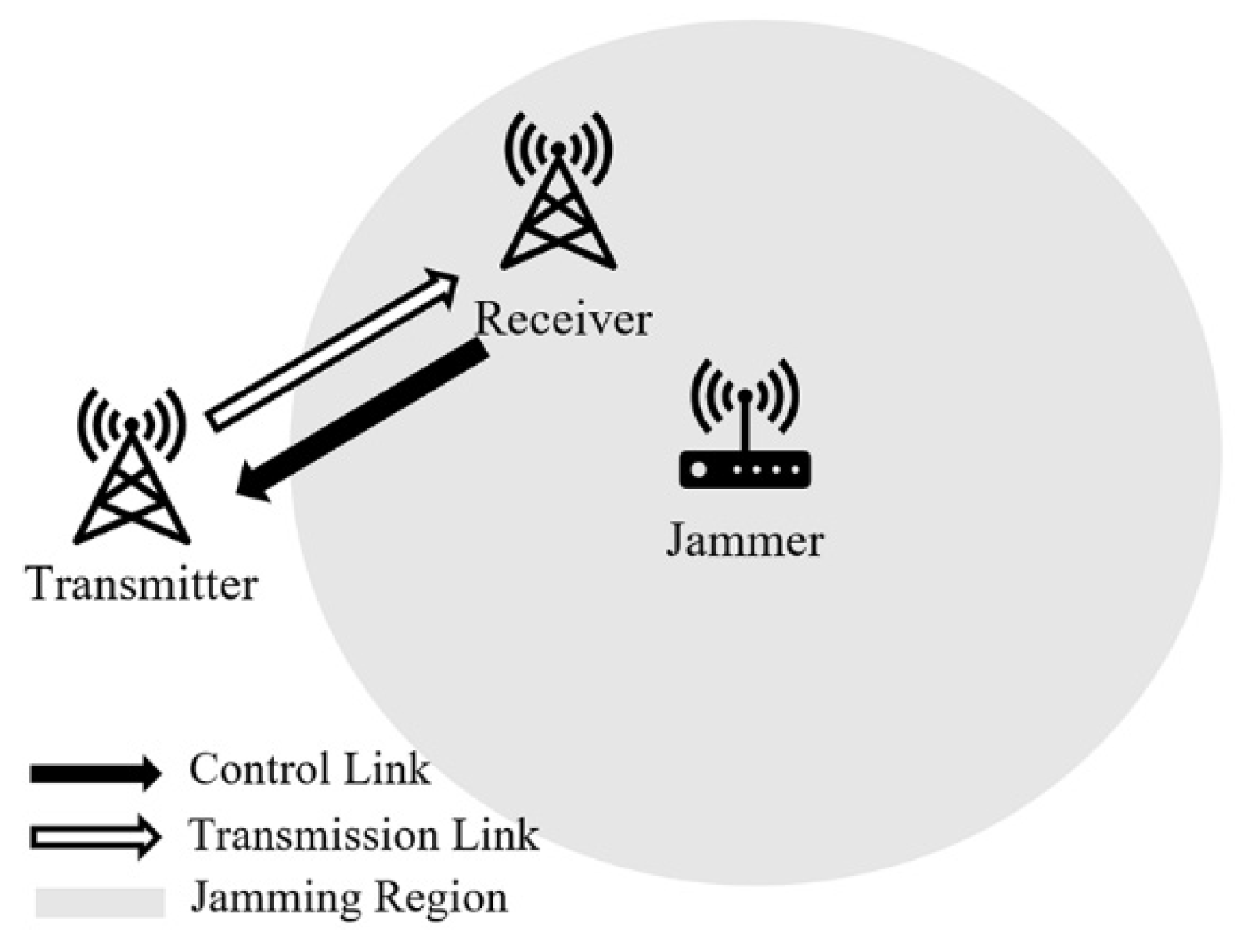
2.1. System Model

As shown in Figure 1, the model in this paper consists of three elements: a legitimate communication transmitter, a corresponding communication receiver, and a malicious jammer whose jamming signal can cover the receiver. For convenience, the following assumptions were made in this study.

• Transmission period: we assume that the time slot with a length of $T_s$ is the smallest unit of continuous transmission. A complete transmission period is composed of $N_T$ continuous time slots. This paper assumes that there are $N_S$ time slots, equivalent to $N_S/N_T$ periods.
• Jammer: we assume that the jammer grasps the information of the transmitter, such as the possible frequency of communication, the width of the time slot, and the transmission period of the wireless communication system, in advance through reconnaissance. The random pulse jamming signal is able to cover the channel of communication completely, and the duration of a single pulse $T_p$ is equal to the length of the communication time slot $T_s$.
• Jamming period: in this paper, the jammer is assumed to set the interference period to be the same as and synchronous with the communication transmission period. It consists of $N_T$ time slots in one period, in which the jammer selects time slot $n_i$ to conduct jamming according to a specific probability distribution. The discrete probability density function is defined as $f_J\left(n\right)$, and the probability of jamming in the $k\mathrm{th}$ period $P_J\left(n_i\right)$ can be expressed as follows:

  $$P_J\left(n_i\right)={\displaystyle \sum }_{i=0}^{\left(k-1\right)N_T·T_s+n_i{T}_s}{f}_J\left(n_i\right)-{\displaystyle \sum }_{i=0}^{\left(k-1\right)N_T·T_s+n_{\left(i-1\right)}{T}_s}{f}_J\left(n_i\right)$$

  (1)

  where $n_iϵ\left[1, N_T\right]$ represents the slot number in one jamming period, and $P_J\left(n_i\right)$ represents the probability that the jammer selects the $n_i\mathrm{th}$ time slot in the $k\mathrm{th}$ period to conduct pulse jamming.

2.2. Problem Formulation

This paper models the problem of anti-random-pulse jamming as a Markov Decision Process (MDP). The definition of the four elements $\left(S,A,P,r\right)$ in the MDP is shown as follows, where $S$ is the state space, $A$ is the action space, $P$ is the state transition probability, and $r$ is the immediate reward that the transmitter can receive from the system.

1.

$S$: The state space is defined as follows:

$$S\triangleq \left\{\left(n_i,j\right):n_i\in \left\{1,2,3\cdots N_T\right\},jϵ\left\{0,1\right\}\right\}$$

(2)

Considering that the state of the environment depends on external malicious interference, we define the state space as a compound variable $s=\left(n_i,j\right)$,$sϵS$, where $n_i$ represents the slot number in a single interference period, and$j$ represents the identification of pulse jamming, i.e., $j=1$ represents the perception of pulse jamming in a single interference period; $j=0$ otherwise.

The principle of the compound variable $\left(n_i,j\right)$ is that $n_i$ records the number of slots and $j$ initializes to 0 in a single interference period. If the transmitter detects pulse jamming in the $n_j\mathrm{th}$ slot, $j$ will keep 1 from the $n_{j+1}\mathrm{th}$ slot to the end of the same period, and $j$ will reset to 0 if next the period starts, which is shown in Figure 2a.

2.

$A$: The action space is defined as follows:

$$A\triangleq \left\{a:aϵ\left\{0,1\right\}\right\}$$

(3)

We define the action that the receiver will perform as a dichotomous problem, i.e., $a=0$ represents the transmitter remaining silent; $a=1$ otherwise.

3.

$P_{s{s}^{\prime }}^a$: $s\times a\times s^{\prime }\to \left[0,1\right]$, whose definition is the probability of transitioning from state $s$ to state $s^{\prime }$ by executing action $a$. Figure 2b shows the state transition of the system, where $P_J\left(n_i\right)$ is the probability of the timeslot selection in Equation (1). For instance, the current state of the timeslot is $s=\left(n_i,j\right)$, and the transmitter performs an action that is required; afterwards, the external environment transitions into the next state $s^{\prime }=\left(n_{i+1},j^{\prime }\right)$. The next sequence number $n_{i+1}$ can be expressed as follows:

$$n_{i+1}=\{\begin{array}{ll}{n}_i+1& n_i<N_T\\ 1& n_i=N_T\end{array}$$

(4)

Obviously, the value of $n_{i+1}$ is related to the current state $n_i$ only.

The next sequence number $j^{\prime }$ can be expressed as follows:

$$j^{\prime }=\{\begin{array}{ll}0& j=0,g=0, n_i<N_T\\ 1& j=0,g=0, n_i<N_T\\ 1& j=1, n_i<N_T\\ 0& n_i=N_T\end{array}$$

(5)

where $g$ represents the consequence of interference, i.e., $g=0$ represents no pulse jamming in the current timeslot and $g=1$ otherwise.

According to the foregoing content, the next state of the environment $s^{\prime }=\left(n_{i+1},j^{\prime }\right)$ is related to the current state $s=\left(n_i,j\right)$ only. So, the system modeled in this paper is Markovian.

Given the above, we define the probability of a state transition $P_{s{s}^{\prime }}^a$ from $s=\left(n_i,j\right)$ to $s^{\prime }=\left(n_{i+1},j^{\prime }\right)$ by a conduction action as follows:

$$P_{s{s}^{\prime }}^a=\{\begin{array}{ll}1& j=1,n_i<N_T or n_i=N_T\\ p_k\left(i\right)& j=0,j^{\prime }=1\&n_i<N_T\\ 1-p_k\left(i\right)& j=0,j^{\prime }=0\&n_i<N_T\end{array}$$

(6)

4.

$r$: The immediate reward function is that the transmitter takes action $a$ in state $s$ to obtain immediate benefits from environmental feedback. According to different states and actions, the following four types of instant reward R in specific scenes are distinguished, and the definition formula is as follows:

$$r\left(s,a\right)=\{\begin{array}{ll}E& j=0,g=0 \mathrm{and} a=1\\ -L& j=0,g=1 \mathrm{and} a=1\\ E& j=1,g=1 \mathrm{and} a=1\\ 0& a=0\end{array}$$

(7)

• If $j=0$, $g=0$, and $a=1$, there is no pulse jamming signal in this interference period and the transmitter conducts the transmission successfully and reaps rewards $E$ from the system.
• If $j=0$, $g=1$, and $a=1$, in this timeslot, a pulse jamming signal appears and the transmitter insists on the transmission, which will be a failure, leading to the loss $L$ from the system.
• If $j=1$, $g=1$, and $a=1$, according to the principle of ‘One period, One pulse’, there will not be a pulse jamming signal in this single period, so the transmitter will perform the transmission successfully and gain the reward $E$.
• If $a=0$, the transmitter remains silent no matter the external environment, and there will be neither a reward nor a loss.

Figure 2c shows the immediate rewards vividly, in which the blue line and the red line in the figure represent the immediate reward situation of the “continuous transmission” and “keep silent” strategies, respectively.

5.

The structure of the timeslot:

This paper divides a single timeslot into three parts chronologically: the conducted action $T_{act}$, the observation $T_{observe}$, and the decision $T_{decide}$.

• $T_{act}$: the transmitter conducts the action that was decided in the last $T_{decide}$.
• $T_{observe}$: the transmitter observes the external environment and senses whether there is a pulse jamming signal right now.
• $T_{decide}$: after updating the Q table, the policy of the next time slot is obtained and transmitted back to the transmitter.

According to the above, the goal of the MDP is to find the optimal strategy ${\pi }^{*}$ corresponding to the maximum long-term cumulative reward under a discount condition. The state-action function (also called the Q value) corresponding to any strategy $\pi$ can be expressed as:

$$Q^{\pi }\left(s,a\right)=E\left\{{\sum }_{\tau =0}^{\infty }{\gamma }^{\tau }{r}_{r+\tau }|s_t=s,a_t=a,\pi \right\}$$

(8)

$Q^{\pi }\left(s,a\right)$ represents the accumulated discount reward that the agent can obtain by executing the action $a$ before using the strategy starting from the corresponding state $s$ at the time $t$. As mentioned above, if the optimal Q values corresponding to all state-action groups are obtained, the optimal strategy ${\pi }^{*}$ can be obtained.

3. SARSA-Based Time-Domain Anti-Jamming Algorithm

This paper proposes a SARSA-based Time-domain Anti-jamming Algorithm (STAA).

When the STAA is in state $s_t$, it will perform the action decided in the last $T_{decide}$, observing the immediate reward $r_t$ and the next state $s_{t+1}$. Therefore, based on the derivation strategy (here set as the ε- greedy strategy), the STAA selects the next action $a_{t+1}$. The principle of updating the Q value is as follows:

$$Q\left(s_t,a_t\right)=\{\begin{array}{ll}Q\left(s_t,a_t\right)+{\alpha }_t\left[r_t+\gamma Q\left(s_{t+1},a_{t+1}\right)-Q\left(s_t,a_t\right)\right],& \mathrm{if} s=s_t,a=a_t\\ Q\left(s_t,a_t\right),& \mathrm{other} \mathrm{cases}\end{array}$$

(9)

In other cases, the Q value remains unchanged. At this point, the STAA has completed one iteration, and it will iterate until the end of the loop. Each complete timeslot corresponds to a complete iteration of the algorithm.

After the completion of initialization, the algorithm repeats the following operations in each full timeslot. According to the policy instruction returned by the receiver at the end of the last timeslot, in sub-slot $T_{act}$ the transmitter performs ‘keep silent’ or ‘transmission’ and calculates the immediate reward $r$ and the probability of the state transition $P_{s{s}^{\prime }}^a$ (line 3). In sub-slot $T_{observe}$, the receiver senses the presence of pulse jamming in the current environment using the perceptual interference technique (line 4). In the decision sub-slot, the receiver deduces the next action according to the update criterion (line 5), and then updates the current Q table according to the equation (line 9). Finally, after receiving the update, the receiver generates the new strategy (line 10) and sends the strategy of the next time slot to the transmitter (line 11). The cycle repeats until the end of the iteration.

In order to achieve a reasonable transition between “dare to explore” at the early stage of decision-making and “rational use” at the later stage of decision-making, closer to the reality of intelligent decision-making, we set $\epsilon =1/\sqrt{t}$, where $t$ represents the number of timeslots (Algorthm 1).

The steps of the STAA are as follows:

Algorthm 1: STAA

Initialize$\alpha$,$\gamma$,$s\in S$,$a\in A$,$Q \left(s,a\right)\leftarrow 0$

$\mathrm{For}$ $t=1,2,\dots T$ $\mathrm{do}$

The transmitter performs $\alpha$ and calculates $r$ and $P_{s{s}^{\prime }}^a$ in sub-slot $T_{act}$

The receiver senses the presence of pulse jamming in sub-slot $T_{observe}$

The receiver deduces the next action according to the update criterion in $T_{decide}$ and the

rule is as follows

The receiver selects the next action $a_{t+1}={\pi }^{\epsilon }\left(s_{t+1}\right)=argma{x}_{aϵA}{Q}_t\left(s_t,a\right)$ with probability $1-\epsilon$

The receiver selects the next action $a_{t+1}=\forall a\in A$ with probability $\mathsf{\epsilon }$

The receiver updates the Q value according to the above formula.

The receiver generates the new strategy

The receiver sends the strategy ($s\leftarrow s_{t+1},a\leftarrow a_{t+1}$) of the next time slot to the transmitter

$end for$

Outputs${\pi }^{*}$

4. Simulation Result and Analysis

4.1. Parameter Settings

We set the parameters related to the simulation in

Table 1. Settings of model-related parameters.

Parameters	Value
$\mathrm{Time} \mathrm{slot} T_s$	0.6 ms
$\mathrm{Sub}-\mathrm{slot} T_{act}$	0.5 ms
$\mathrm{Sub}-\mathrm{slot} T_{observe}$	0.04 ms
$\mathrm{Sub}-\mathrm{slot} T_{decide}$	0.06 ms
$\mathrm{Learning} \mathrm{parameter} \alpha$	0.8
$\mathrm{Discount} \mathrm{parameter} \gamma$	0.6
$\mathrm{Greedy} \mathrm{index} \epsilon$	$1/\sqrt{t}$
$\mathrm{Transmission} \mathrm{reward} E$	1
$\mathrm{Transmission} \mathrm{loss}-L$	−3
$\mathrm{The} \mathrm{total} \mathrm{number} \mathrm{of} \mathrm{time} \mathrm{slots} N_S$	10,000
$\mathrm{The} \mathrm{number} \mathrm{of} \mathrm{time} \mathrm{slots} \mathrm{in} \mathrm{one} \mathrm{period} N_T$	10

as follows:

This paper proposes a SARSA-based Time-domain Anti-jamming Algorithm (STAA).

When the STAA is in state $s_t$, it will perform the action decided in the last $T_{decide}$, observing the immediate reward $r_t$ and the next state $s_{t+1}$. Therefore, based on the derivation strategy (here set as the ε- greedy strategy), the STAA selects the next action $a_{t+1}$. The principle of updating the Q value is given in Equation (9).

In order to evaluate the performance of the proposed algorithm, this section compares the performance of the proposed algorithm with that of the following two transmission schemes:

• Continuous Transmission (CT): the transmitter continues to send data to the receiver without taking any anti-interference measures;
• The Time Domain anti-jamming Algorithm (TDAA) based on Q-learning: the anti-jamming algorithm based on Q-learning is used by the transmitter to cope with external interference and realize data communication with the receiver. For a detailed description of the algorithm, see [11].

It is worth mentioning that although Q-learning and SARSA are both reinforcement learning algorithms, they differ from each other, especially in terms of the iteration strategy. Figure 3 vividly shows the difference in the iteration strategy between Q-learning and SARSA. Q-learning’s strategy is to try possible actions in each iteration, select the prescribed action with the highest immediate return with the probability of $1-\epsilon$, and try actions randomly in the other cases. It is easier to obtain the optimal action quickly at the beginning of the iteration, but the high risk brought about by the high returns makes the TDAA fluctuate easily. SARSA, on the other hand, is more inclined to choose the safe and conservative strategy. The differences in the two core strategies suggest that the STAA will perform better in terms of stability and reliability than the TDAA.

In order to investigate the performance of the STAA and compare the two schemes, we set the following four indicators to investigate the survival ability, the transmission stability, and the learning of the anti-jamming algorithm, respectively.

• Final Collision Rate of Jamming (FCRJ). Firstly, we define the collision rate of jamming ${\rho }_j\left(k\right)$, where ${\rho }_j\left(k\right)={\tau }_{jam}^W\left(k\right)/\left(N_T·W\right)$, which is used to describe the change in the collision probability of transmission and pulse jamming in each interference period, where ${\tau }_{jam}^W\left(k\right)$ represents the number of timeslots that are jammed in the $k\mathrm{th}$ interference period when iterating $W$ times.$W$ represents the number of iterations that the STAA performed; in this paper, we set it to 1000. Finally, we select the final value of the collision rate of jamming, the so-called FCRJ, at the end of an iteration, which is used to describe the algorithm’s ability to survive when jammed.
• Average Reward in Each Period (AREP). Firstly, we define the cumulative rewards $R_k$ in a single period. $R_k,=\left(E·{\tau }_{trans}^W\left(k\right)+\left(-L\right)·{\tau }_{jam}^W\left(k\right)\right)$. Further, we define the average reward $R_{average}$ in each period, where $R_{average}=\sum _{k=1}^W{R}_k/k$, $k\in \left\{1,2,3\cdots W\right\}$, which is used to describe the algorithm’s transmission ability after the $k\mathrm{th}$ interference period.
• Dynamic Fluctuation Ratio (DFR). To describe the stability during transmission, we define $F=\left(R_{k+5}-R_k\right)/\left(\sum _{n=k}^{k+5}{R}_k\right)$, where $kϵ\left\{1,2.3\cdots \cdots W-5\right\}$, which is used to describe the algorithm’s degree of fluctuation during transmission.
• Velocity of Learning Anti-jamming (VLA). In this paper, we define $v=N_{episode}/N_{pre-stablize}$, where $N_{episode}=N_S/N_T$. $N_{pre-stablize}$ is the number of pre-stable disturbance periods of dynamic fluctuations, which is used to describe how fast the algorithm learns external disturbances.

Last, but not least, the distribution of the pulse jamming selection is a vital parameter. We set the jamming selection to have a normal distribution. The probability density function $f_J\left(t\right)$ in the $k\mathrm{th}$ period can be expressed as follows:

$$f_J\left(t\right)=\frac{1}{\sqrt{2\pi }\sigma }\exp \left[-\frac{{\left(t-\mu \right)}^2}{2{\sigma }^2}\right]$$

(10)

To ensure a normal distribution in the corresponding interference period with respect to the median axis symmetry, the value of the mathematical expectation $\mu$ can be expressed as follows:

$$\mu =\left(k-\frac{1}{2}\right)N_T·T_s+{\tau }_0{T}_s$$

(11)

where ${\tau }_0$ is the number of timeslots when the jammer starts to work. As the other element in the normal distribution ${\sigma }^2$, to make sure that the probability distribution of pulse jamming can strictly correspond to each jamming cycle, that is, the $k\mathrm{th}$ pulse interference falls within the $k\mathrm{th}$ interference cycle, we set $\sigma =\left(N_T·T_s\right)/10$ according to the Pauta Criterion.

According to the above two factors, the probability of pulse interference occurring in the $n_i$ timeslot of the $k\mathrm{th}$ interference cycle can be expressed as follows:

$$P_J\left(n_i\right)={{\displaystyle \int }}_{k{N}_T{T}_s+n_i{T}_s}^{k{N}_T{T}_s+(n_i+1)T_s}\frac{1}{\sqrt{2\pi }\sigma }\exp \left[-\frac{{\left(t-\mu \right)}^2}{2{\sigma }^2}\right]dt$$

(12)

Figure 4 shows the schematic diagram of the probability distribution of time slot interference.

4.2. Analysis of Simulation

4.2.1. Basic Analysis of Indicators

Through the above-described background settings, the collision rate of jamming and the average reward in each period of continuous transmission of the STAA and the TDAA with a normal distribution of random pulse interference in the time domain were compared.

Figure 5 shows that the STAA can effectively reduce the probability of interference collision, which is much lower than the probability of random pulse interference (0.1) within the interference cycle, and the decreasing trend is similar to that of the TDAA. As shown in Figure 6, the STAA steadily improved its throughput, ranking among the top three in performance.

In conclusion, the comparison between the collision rate and average cycle return of the three algorithms shows that the STAA has good anti-interference performance and anti-interference transmission performance in this situation.

Figure 6 shows that the AREP curves of the TDAA and STAA both have a decrease in performance at the beginning of the iteration, and then the AREP steadily increases. Local values are magnified, and it was found that the local maximum of performance decline could be uniformly defined as the “Peak Value of Return (PVR)” in this paper. The local minimum was defined as the “Valley Value of Risk” (VVR), and the interval from the PVR to the VVR was called the “Trap of Return”. The reward trap is the performance fluctuation inevitably caused by trial and error in the process of making the optimal decision at the beginning of the iteration, and the absolute difference between the PVR and the VVR of the STAA is larger than that of the TDAA. Therefore, the TDAA in local areas is more volatile and unstable.

From local areas to the entire area, fluctuations in the TDAA and STAA in Figure 6 can be observed. It was found that with the increase in the number of interference cycles, both the TDAA and the STAA experienced a period of violent fluctuations and entered a relatively stable fluctuation interval, which was denoted the “Dynamic Stability Interval” in this paper. Taking this case as an example, it was found that the range of the dynamic fluctuation interval (DSI) was about $\left[-0.1 , 0.1\right]$. In Figure 7, the $N_{pre-stablize}$ of each algorithm is marked on the X-axis, and it was found that the TDAA can enter the dynamic stability interval earlier than the STAA. As the total number of interference cycles is fixed, the learning speed V is inversely proportional to $N_{pre-stablize}$, so the TDAA has better performance than the STAA in learning the features of the external interference. We calculated the fluctuation value after the DSI and plotted it in a frequency diagram to observe the transmission stability performance as shown in Figure 8.

4.2.2. Risk–Return Ratio $\mathsf{\omega }$

The results show that, compared with the TDAA, the fluctuation value of the STAA is more concentrated near the fluctuation value of zero, and the number of unstable fluctuation values exceeding the DSI is less than that of the TDAA. Therefore, the STAA is more stable than the TDAA in terms of transmission performance.

Considering the impact of external interference risks on the performance of the algorithm model, the concept of the risk–benefit ratio [15] is introduced and we define $\omega$ as follows:

$$\omega =L/E$$

(13)

We set $\omega =1/4,1/2,1,2,4$, respectively, where $\omega =1$ is the reference value. Here, we analyze the consequences of the compared performance when the STAA and the TDAA face different degrees of the risk–return ratio $\omega$.

4.2.3. Simulation under Different $\mathsf{\omega }$ Conditions

The simulation results of each performance index are shown in

Table 2. Performance of the TDAA [11] and the STAA under different ω conditions.

ω	ALGORITHM	FCRJ (%)	VLA	AREP	$\mathbf{DVR} \left({10}^{-5}\right)$
1/4	TDAA	9.54	12.35	8.57	3.61
	STAA	9.15	9.09	8.58	2.16
1/2	TDAA	8.52	15.38	8.35	7.43
	STAA	5.27	10.42	8.40	6.25
1	TDAA	4.38	17.86	8.10	26.20
	STAA	4.76	16.13	8.12	20.01
2	TDAA	1.59	26.32	7.81	61.72
	STAA	1.84	18.52	7.78	46.85
4	TDAA	0.69	43.48	7.28	111.33
	STAA	0.78	22.73	7.25	104.66

, and a schematic diagram of the performance comparison is shown in Figure 9. In order to verify the STAA’s excellent performance in stable transmission, a diagram comparing the numerical fluctuation frequency under five ω conditions was made and is shown in Figure 9 and Figure 10.

It can be observed from Figure 9 and Figure 10 that the STAA, which has a more conservative iteration strategy, has a narrower fluctuation range and a more concentrated fluctuation value than the TDAA [11], which has a more radical iteration strategy, regardless of whether $\omega$ ≤ 1 or $\omega$ ≥ 1. This is consistent with the conclusion of the initial simulation.

Subsequently, the performance indicators of the TDAA and STAA under different $\omega$ conditions were simulated. The values are shown in Table 2, and a schematic diagram of the performance comparison is shown in Figure 11. It is worth noting that the values of those indicators shown in Table 2 are pure numbers with no units according to the definitions above.

An additional verification of the fluctuation confirmed our idea. The final comparison results are consistent with the above conclusions. It was observed that the STAA achieved good communication transmission on the basis of maintaining small fluctuations under different $\omega$ conditions. In particular, under a high risk of interference, the advantages of small fluctuations and high-quality transmission are obvious.

5. Conclusions

In this paper, we proposed a SARSA-based Time-domain Anti-jamming Algorithm (STAA) for countering random pulse jamming in the time domain. By comparing the FCRJ, AREP, DVR, and VLA, the simulation results show that the STAA has small fluctuations, a high degree of determinacy, and good stability. Finally, through the control variable (the risk–benefit ratio ω), an experiment analyzing the performance of the STAA and the TDAA under different risk scenarios was carried out. The simulation shows that in terms of the stability of transmission, the STAA performs better than the TDAA. As the ω changes, its fluctuation range decreases by 6.0% to 40.2% compared with the TDAA, and its transmission performance error compared with the TDAA is between −0.4% and 0.6%, which can be ignored. Hence, the STAA’s value lies in its stable transmission and low volatility during periods of high demand. The simulation results further prove that, under the same interference risk conditions, the STAA’s transmission performance is more stable and less volatile than that of the TDAA. This is due to its tendency to choose conservative strategies when iterating. However, it should be noted that the cost of the stability of the STAA is the lack of an ability to extract more valuable strategies from iterations, which is not the case for the TDAA, resulting in latency in the process of learning the optimal strategy. Our conclusion is that the STAA is much more conservative than the TDAA in terms of iteration strategies. Overall, although the strategy of the STAA is more conservative, the indicators show that the STAA is more stable and reliable, especially in situations where the risk of interference is high.

References

1. Sampath, A.; Hui, D.; Zheng, H.; Zhao, B.Y. Multi-channel Jamming Attacks using Cognitive Radios. In Proceedings of the 2007 16th International Conference on Computer Communications and Networks, Honolulu, HI, USA, 13–16 August 2007. [Google Scholar]
2. Lee, J.J.; Lim, J. Effective and Efficient Jamming Based on Routing in Wireless Ad Hoc Network. IEEE Commun. Lett. 2012, 16, 1903–1906. [Google Scholar] [CrossRef]
3. Noels, N.; Moeneclaey, M. Performance of advanced telecommand frame synchronizer under pulsed jamming conditions. In Proceedings of the 2017 IEEE International Conference on Communications (ICC), Paris, France, 21–25 May 2017. [Google Scholar]
4. Busoniu, L.; Babuska, R.; Schutter, B.D. A Comprehensive Survey of Multiagent Reinforcement Learning. IEEE Trans. Syst. Man Cybern. Part C 2008, 38, 156–172. [Google Scholar] [CrossRef] [Green Version]
5. Slimeni, F.; Chtourou, Z.; Scheers, B.; Nir, V.L.; Attia, R. Cooperative Q-learning based channel selection for cognitive radio networks. Wirel. Netw. 2018, 25, 4161–4171. [Google Scholar] [CrossRef]
6. Wang, B.; Wu, Y.; Liu, K.J.R.; Clancy, T.C. An Anti-Jamming Stochastic Game for Cognitive Radio Networks. IEEE J. Sel. Areas Commun. 2011, 29, 877–889. [Google Scholar] [CrossRef] [Green Version]
7. Xiao, L.; Lu, X.; Xu, D.; Tang, Y.; Wang, L.; Zhuang, W. UAV Relay in VANETs Against Smart Jamming with Rein-forcement Learning. IEEE Trans. Veh. Technol. 2018, 67, 4087–4097. [Google Scholar] [CrossRef]
8. Aref, M.A.; Jayaweera, S.K. A cognitive anti-jamming and interference-avoidance stochastic game. In Proceedings of the 2017 IEEE International Conference on Cognitive Informatics & Cognitive Computing (ICCI*CC), Oxford, UK, 26–28 July 2017. [Google Scholar]
9. Machuzak, S.; Jayaweera, S.K. Reinforcement learning based anti-jamming with wide-band autonomous cognitive radios. In Proceedings of the 2016 IEEE/CIC International Conference on Communications in China (ICCC), Chengdu, China, 27–29 July 2016. [Google Scholar]
10. Aref, M.A.; Jayaweera, S.K.; Machuzak, S. Multi-Agent Reinforcement Learning Based Cognitive Anti-Jamming. In Proceedings of the 2017 IEEE Wireless Communications and Networking Conference (WCNC), San Francisco, CA, USA, 19–22 March 2017. [Google Scholar]
11. Zhou, Q.; Li, Y.; Niu, Y. A Countermeasure Against Random Pulse Jamming in Time Domain Based on Reinforcement Learning. IEEE Access 2020, 8, 97164–97174. [Google Scholar] [CrossRef]
12. Lilith, N.; Dogancay, K. Dynamic channel allocation for mobile cellular traffic using reduced-state reinforcement learning. In Proceedings of the Wireless Communications & Networking Conference, Atlanta, GA, USA, 21–25 March 2004. [Google Scholar]
13. Lilith, N.; Dogancay, K. Distributed reduced-state SARSA algorithm for dynamic channel allocation in cellular networks featuring traffic mobility. In Proceedings of the IEEE International Conference on Communications, Seoul, Korea, 16–20 May 2005. [Google Scholar]
14. Wang, W.; Kwasinski, A.; Niyato, D.; Han, Z. A Survey on Applications of Model-Free Strategy Learning in Cognitive Wireless Networks. IEEE Commun. Surv. Tutor. 2016, 18, 1717–1757. [Google Scholar] [CrossRef]
15. Lintner, J. The valuation of risk assets and the selection of risky investments in stock portfolios and capital budgets. Stoch. Optim. Models Financ. 1969, 51, 220–221. [Google Scholar] [CrossRef]
Figure 1. Schematic diagram of the system model.
Electronics 11 01456 g001
Figure 2. Schematic diagram of the elements in this model. (a) Schematic diagram of the state parameters; (b) State transition diagram; (c) Diagram of the immediate reward function; (d) Schematic diagram of the time slot structure.
Electronics 11 01456 g002
Figure 3. Schematic diagram of the differences in the iteration strategies. (a) SARSA’s iteration strategy; (b) Q-learning’s iteration strategy.
Electronics 11 01456 g003
Figure 4. Schematic diagram of the probability distribution of timeslot interference.
Electronics 11 01456 g004
Figure 5. Schematic diagram comparing the CRJ between continuous transmission (CT), the TDAA [11], and the STAA.
Electronics 11 01456 g005
Figure 6. Schematic diagram comparing the AREP between continuous transmission (CT), the TDAA [11], and the STAA.
Electronics 11 01456 g006
Figure 7. Schematic diagram comparing the DFR between the TDAA [11] and the STAA.
Electronics 11 01456 g007
Figure 8. Schematic diagram comparing the numerical fluctuation frequency in the DSI between the STAA and the TDAA [11] (red represents the STAA and blue represents the TDAA [11]).
Electronics 11 01456 g008
Figure 9. Schematic diagram comparing the numerical fluctuation frequency in the DSI under ω 1 : (a) ω = 1 / 4 ; (b) ω = 1 / 2 ; (c) ω = 1 (red represents the STAA and blue represents the TDAA [11]).
Electronics 11 01456 g009
Figure 10. Schematic diagram comparing the numerical fluctuation frequency in the DSI under ω 1 : (a) ω = 1 ; (b) ω = 2 ; (c) ω = 4 (red represents the STAA and blue represents the TDAA [11]).
Electronics 11 01456 g010
Figure 11. Schematic diagram of the performance comparison under different ω conditions between the TDAA [11] and the STAA. (a) The contrast between the VLA and FCRJ; (b) The contrast between the AREP and DVR.
Electronics 11 01456 g011