Short-Term Traffic-Flow Forecasting Based on an Integrated Model Combining Bagging and Stacking Considering Weight Coefficient

Abstract

This work proposed an integrated model combining bagging and stacking considering the weight coefficient for short-time traffic-flow prediction, which incorporates vacation and peak time features, as well as occupancy and speed information, in order to improve prediction accuracy and accomplish deeper traffic flow data feature mining. To address the limitations of a single prediction model in traffic forecasting, a stacking model with ridge regression as the meta-learner is first established, then the stacking model is optimized from the perspective of the learner using the bagging model, and lastly the optimized learner is embedded into the stacking model as the new base learner to obtain the Ba-Stacking model. Finally, to address the Ba-Stacking model’s shortcomings in terms of low base learner utilization, the information structure of the base learners is modified by weighting the error coefficients while taking into account the model’s external features, resulting in a DW-Ba-Stacking model that can change the weights of the base learners to adjust the feature distribution and thus improve utilization. Using 76,896 data from the I5NB highway as the empirical study object, the DW-Ba-Stacking model is compared and assessed with the traditional model in this paper. The empirical results show that the DW-Ba-Stacking model has the highest prediction accuracy, demonstrating that the model is successful in predicting short-term traffic flows and can effectively solve traffic-congestion problems.

1. Introduction

In recent years, as the economy has grown and people’s quality of life has improved, people’s demands for transportation has increased, and vehicles have progressively become the preferred mode of transportation. However, this has caused an increase in traffic congestion, and a contradiction and an intensification between the supply and demand of road traffic. As a result, comprehensive technologies and methods are urgently needed to properly control and monitor traffic flow, as well as to alleviate traffic congestion and other issues.

Traffic-flow prediction is fundamental in traffic management and dredging, and its accuracy is critical in resolving traffic-congestion issues. A vast number of experts have done extensive research on this in recent years, primarily utilizing a linear or nonlinear model to predict the following:

(1)

Linear model

The historical average forecasting methods, the time series forecasting methods, and the Kalman wave forecasting methods were all used in the early days of traffic flow research. Some scholars use simple linear models to predict traffic flow, such as the autoregressive moving average model (ARIMA) model, which is suitable for predicting data with time rules, but the traffic flow has a strong non-linear trend, and its prediction accuracy for traffic flow is not high and has limitations [1,2,3]. D. Cvetek et al. used the collected data to compare some common time series methods such as ARIMA and SARIMA, showing that the ARIMA model provides better performance in predicting traffic demand [4].

The Kalman wave is also used as a linear theory-prediction method by many scholars. Okutani firstly applied the Kalman wave to traffic-flow forecasting [5]. According to the inherent shortcomings of Kalman wave variance, Guo et al. proposed an adaptive Kalman wave energy update variance, which improved the prediction performance of the original model [6]. Israr Ullah et al. developed an artificial neural network (ANN)-based learning module to improve the accuracy of the Kalman filter algorithm [7]. Additionally, in the experiment of the indoor environment prediction in the greenhouse, good prediction results were obtained. Therefore, the Kalman wave model can effectively reduce the uncertainty and noise in the flow change in the prediction process, but it is difficult to predict the nonlinear change trend of the traffic flow.

(2)

Non-linear model

With the recent development of technology, the widespread use of powerful computer and mathematical models is applied to this field [8]. Among them, the wavelet neural network, as a representative of the nonlinear theoretical model, has a better traffic-flow prediction effect. Gao et al. used the network model to predict short-term traffic flow and achieved good results [9]. Although the wavelet neural network converges faster and the prediction accuracy is higher, the existence of the wavelet basis function increases the complexity of the model.

Machine learning models have become research hotspots that have been widely used in many fields. They are best applied to the field of traffic flow. Qin et al. proposed a new SoC estimation method on the impact of temperature on SoC estimation, and the use of limited data to rapidly adjust the estimation model to new temperatures, which not only reduces the prediction error at a fixed temperature but also improves the prediction accuracy at a new temperature [10]. Xiong Ting et al. used the random forest model to predict the traffic flow and achieved high prediction accuracy, based on the combination of spatio-temporal features [11]. Lu et al. used the XGBoost model to predict the traffic flow at public intersections in Victoria and achieved high prediction accuracy [12]. Alajali et al. used the GBDT model to analyze the lane-level traffic flow data on the Third Ring Road in Beijing on the basis of feature processing and proved that the model has a good prediction effect and is suitable for the traffic prediction of different lanes [13]. On the basis of extracting features, Yu et al. used the KNN model to complete the prediction of the traffic node and route traffic flow, which achieved good prediction results [14].

Therefore, it can be concluded that the integrated model based on the decision tree is widely used and has high prediction accuracy, while the KNN model can eliminate the sensitivity to abnormal traffic flow in the prediction. Qin et al. proposed a slow-varying dynamics-assisted temporal CapsNet (SD-TemCapsNet) that introduced a long short-term memory (LSTM) mechanism to simultaneously learn slow-varying dynamics and temporal dynamics from measurements, achieving an accurate RUL estimation [15]. Although LSTM has been used by many scholars as a network model with high accuracy in terms of time series prediction, the complexity of the network itself is difficult to avoid. The gate recurrent unit model (GRU) can effectively solve this problem, which can complete the prediction of traffic with fewer parameters under the premise of meeting a certain prediction accuracy. Dai et al. used the GRU model to predict the traffic flow under the condition of making full use of the features and verified the effectiveness of the model through comparative analysis with the convolutional neural network [16]. As an evolutionary model of LSTM, the GRU can predict traffic flow with fewer parameters, under the premise of satisfying a certain prediction accuracy.

Although machine learning models perform well in traffic-flow prediction, the prediction performance of the single model is limited. Therefore, a model combining multiple single models has gradually become a trend [17]. Pengfei Zhu et al. integrated the GRU and BP to predict the frequency shift of unknown monitoring points, which effectively improved the prediction accuracy of a single model [18]. Although the above combined models can improve the accuracy to a certain extent, they are limited by the number of single models. The integrated model that mixes multiple models is gradually becoming favored by scholars and has been applied to various fields [19]. Shuai Wang et al. proposed a probabilistic approach using stacked ensemble learning that integrates random forests, long short-term memory networks, linear regression, and Gaussian process regression, for predicting cloud resources required for CSS applications [20]. Common ensemble models include bagging [21], boosting [22], and stacking [23]. Compared with other ensemble models, the stacking model has a high degree of flexibility, which can effectively integrate the changing characteristics of heterogeneous models to make the prediction results better.

In summary, the single prediction model has limitations, and the combined forecasting model has gradually become a trend. Common models that can integrate a single model include the entropy combination method, the inverse error group method, the ensemble learning method, and other combination methods. [24,25]. Among them, the comprehensive model is more practical. The bagging integration model and the boosting integration model, generally used for a homogeneous single model, are limited to a single model, while the stacking integration model is more commonly used for the fusion of heterogeneous models. Therefore, the first use of the bagging model is to optimize the base learner model and then optimize the stacking model, to improve the overall performance of the model.

2. Establishment of the DW-Ba-Stacking Model

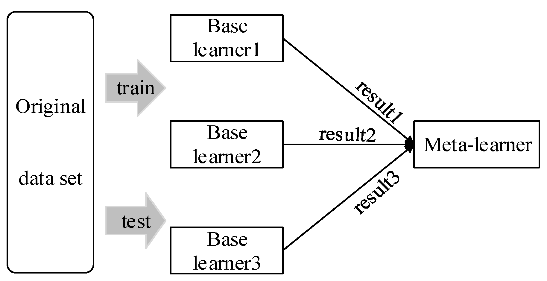
In this section, a DW-Ba-Stacking model was put forwarded in detail. The DW-Ba-Stacking model consists of three parts in total, the stacking model (stacking), the bagging model (Ba), and the dynamic weighting adjustment (DW).

2.1. Stacking Model

Traffic flow trends are complex, and there are various models used in this field, among which machine learning models are widely used in traffic-flow prediction due to their good non-linear fitting. In order to obtain a stacking model with high accuracy, machine learning models with different merits and good applications in this field are selected for fusion: the random forest model, which is less prone to overfitting; the KNN model, which is insensitive to outliers; the decision-tree model; the XGBoost and GBDT models; the GRU model, which can effectively use temporal features; and the K-fold cross validation to prevent overfitting.

2.1.1. Principle of the Stacking Model

The stacking model obtains the final prediction by linear or non-linear processing of the sub-learners. The main principle is that the original data are first predicted by the base learner, and then the prediction is passed to the meta-learner to obtain the final result. To prevent overfitting, the data are usually trained by $K$ fold cross-validation, as follows.

Let the original data set $M=\{(y_n,x_n)\}$, $x_n$ be the feature variables of the $n$ sample, $y_n$ be the predictor variables of the $n$ sample, and the number of base learners be $L$ The data from the original dataset $1/K$ are used as the validation set, $M_{1/k}$; the rest of the data $M^{-1/k}=M-M_{1/k}$ are used as the training set; the divided data are fed into the base learner $A_L^{-1/k}$ for training, and the prediction results from $K$ are obtained $N_{kL}$. The predictions from the base learner and $y_n$ are then used as the training set for the meta-learner, which trains the model and makes predictions.

2.1.2. Machine Learning Models

Random Forest and KNN Models

The Random Forest model is a modified bagging algorithm. When the model is used for regression, the single model that is integrated is the CART regression tree. First, samples are drawn by bootstrap sampling with replacement; then, the corresponding regression trees are modelled for the m different samples drawn to form the forest; and, finally, the average of the predictions from the different regression trees is taken as the final prediction. The samples and features of the regression trees in the model are chosen randomly. Each regression tree built through bootstrap sampling is independent and uncorrelated. This feature increases the variation between models and enhances the generalization ability of the model. At the same time, the random nature of feature selection reduces the variability of the models. As the number of regression trees increases, the model error gradually converges, which reduces the occurrence of overfitting. This is why the model was selected as one of the base learners.

When the KNN model is used for classification, it determines the k sample types by searching for k samples in the historical data that are similar to the samples to be classified. The principle can be expressed as follows:

$$S=\left(X_1,Y_1\right),\left(X_2,Y_2\right) \dots \left(X_N,Y_N\right)$$

(1)

where $X$ is the feature vector, $Y$ is the category of the example sample, and $i=\left(1,2,3\dots ,N\right)$. The Euclidean distance is used to express the similarity between the sample to be classified and the feature sample in $S$. The Euclidean distance between the observed sample and the feature is calculated. Based on the calculated distances, find the closest K points to the object to be classified in S and determine the X category. The principle is shown in Figure 1. There are $N$ samples with the categories $Q_1,Q_2,\dots ,Q_N$, which are $N$ different categories. By testing the Euclidean distance between sample $X_i$ and the $N$ training sets, M samples that are closer to sample $X_i$ are obtained, and if most of the $M$ samples belong to a certain type, then sample $X_i$ also belongs to that type. The model can be applied to both discrete and continuous features and is insensitive to outliers, so it is used as a base learner.

Decision Trees, and the GBDT and XGBoost Models

A decision tree is a model consisting of nodes and directed edges that allow predictions to be made by correspondence between attributes and objects. The internal nodes are the features of the object and the leaf nodes are the classes of the object. The model has a wide range of applications, and it is efficient and suitable for high-dimensional feature processing, which is why it has been chosen as one of the traffic-flow prediction models. It aims to summarize certain rules from the training dataset and eventually achieve the correct result. The essence is to find the optimal decision tree. The three more important features in the search process are attribute selection, decision tree generation, and decision tree pruning. The key to their generation is the division of the optimal attributes. Purity is a measure based on the assignment of attributes. The evaluation metrics for measuring purity include information gain, gain rate, and Gini index. The principle is shown in Figure 2.

Both GBDT and XGBoost are algorithms that evolve by boosting. GBDT is formed by continuously fitting the residual error by updating the learners on the gradient. When the residual error reaches a certain limit, the model stops iterating and forms the final learner. The model can be very good at fitting non-linear data. However, the computational complexity will increase when the dimensionality is high and the traffic flow has fewer characteristic dimensions, so the model is suitable for prediction in this area. The regulator model is a linearly weighted combination of different regulators.

$$F_n\left(x\right)={\displaystyle \sum }_{n=1}^{N}R(x;{\theta }_n)$$

(2)

where $T(x;{\theta }_n)$ is a weak regressor. The loss function of the weak regressor is

$${\widehat{R}}_n=argmin{\displaystyle \sum }_{i=1}^{M}L(y_i,F_{n-1}\left(x_i\right)+T(x;{\theta }_n))$$

(3)

where $L\left(\cdot \right)$ is the loss function.

XGBoost and GBDT share the same principles and integrated model, with a process of continuously fitting the residuals and gradually reducing them. During the fitting process, the learner is updated with first-order derivatives and second-order derivatives. Specifically, the second-order Taylor expansion of the loss function and the positive term of the error component are used as the objective function during each round of iterations. It updates the parameters through the solution of the least significant graph. The positive term in the objective function controls the complexity of the model, reduces the variance of the model, and makes the learning process of the model easier, so this model is chosen as the base learner. The loss function L is

$$L={\displaystyle \sum }_{i=1}^{M}l(y_i,{\widehat{y}}_i)+{\displaystyle \sum }_{n=1}^N\Omega (f_k)$$

(4)

In the formula, the first half is the error between the predicted and actual values; the second half is the conventional term.

$$\Omega \left(f\right)=\gamma T+\frac{1}{2}\lambda {\Vert \omega \Vert }^2$$

(5)

The Equations$\gamma$ and $\lambda$ are the penalty coefficients for the model.

GRU Model

A deep-learning model is one of the machine learning models. It can adapt well to the changing characteristics of data when the amount of data is appropriate. It has gradually been applied to various fields with good results. Zheng Jianhu et al. relied on deep learning (DL) to predict traffic flow through a time series analysis and carried out long-term traffic-flow prediction experiments based on the LSTM network-based traffic-flow prediction model, the ARIMA model, and the BPNN model [26]. It can be seen that regular sequences have won the favor of various scholars and that GRU is a more mature network for processing time series in recent years. Additionally, the earliest proposed network to deal with time series is RNN, but it is prone to gradient disappearance, leading to network performance degradation. Zhao et al. used long short-time memory (LSTM) to predict traffic flow under the premise of considering spatial factors in the actual prediction process and achieved high prediction accuracy [27], but the network model also has the disadvantage of poor robustness. In order to solve this problem, Li Yuelong et al. realized the optimization of the prediction performance of the network through the network space feature fusion rights protection unit [28]. It can be seen that although LSTM is used by many scholars as a network model with high time series prediction accuracy, the complexity of the network itself is difficult to avoid. The GRU model, on the other hand, can effectively reduce the network parameters while ensuring the performance of the model itself. Its structure is shown in Figure 3.

$$r_t=\sigma \left(W_r{x}_t\times U_r{h}_{t-1}+b_r\right)$$

(6)

$$z_t=\sigma \left(W_z{x}_t\times U_z{h}_{t-1}+b_z\right)$$

(7)

$${\tilde{\mathit{h}}}_t=\mathit{tan}\mathit{h}(W_{\mathit{h}}{x}_t+U_{\mathit{h}}\left({\mathit{h}}_{t-1}\otimes r_t\right)+b_r)$$

(8)

$${\tilde{\mathit{h}}}_t=\left(1-z_t\right)\otimes {\mathit{h}}_{t-1}+z_t\otimes {\tilde{\mathit{h}}}_t$$

(9)

where $\otimes$ is the product of the corresponding positions of the two matrices, $\sigma$ is the activation function, $W$ and $U$ are the weight parameters of the network, and $b$ is the bias parameter of the network, which is the state value of the hidden layer at different moments. The reset gate $r_t$ determines the input ratio of the previous state information ${\mathit{h}}_{t-1}$ to the current network cell; the update gate $Z_t$ determines the deletion ratio of the previous state information. The entire network cell is filtered by the two gates to determine the valid information of the network cell. Compared with the LSTM model, the GRU model reduces one gate unit and only sets the reset gate and update gate to control the input and output information of the network unit, which reduces the complexity of the network and improves the network training speed.

2.2. Bagging Model

The overall architecture of the Ba-Stacking model included the bagging model processing stage and the stacking model processing stage. Because the bagging was only embedded as part of the stacking model, the stacking model architecture plays a big role. The more important processing phases are: the base learner processing phase and the meta learner processing phase. The base learner processing stage requires different base learners to obtain the prediction results, so the choice of the base learner plays an important role. The meta-learner processing stage is more important because it includes a large amount of raw data information, so it is important that the effect of using the base learner information affects the final prediction results. However, the output information of different base learners is duplicated, and the data variability is not strong enough to extract the effective information of the output data. Therefore, to address the problem that the output information of base learners cannot be fully utilized, it is necessary to consider how to effectively utilize its output information and reflect its importance and variability.

To further improve the stacking model, this paper considers the use of the bagging algorithm to further optimize the base learner and reduce the base learner variance, as two ways to improve the potential performance of the meta-learner model in the stacking model.

Considering that the prediction effect of the base learner directly affects the final effect of the integrated model, the prediction effect of the base learner of the stacking-integrated model is optimized by the bagging algorithm. To better extract the base learner features, a ridge regression with linearity is used as the meta-learner, and the overall construction principle is shown in Figure 4.

The process of this model is to optimize the data features of the stacking base learner based on its output information through the bagging algorithm and then further input this optimized data into the meta-learner in the stacking-integrated model for traffic prediction. The process consists of three parts: the first part builds the stacking base learner model by comparing and analyzing different features to obtain the optimal base learner model; the second part builds the stacking model and obtains the optimal stacking model by comparing and analyzing different base learner models and meta-learner models; finally, the bagging model is combined into the stacking model to build the Ba-Stacking model.

2.3. DW Model

The entropy value can be expressed as the uncertainty of each value. The entropy weighting method in the tradition weights the fixed coefficients of each model, but the certainty degree of different positions of the base learner can be deduced from the certainty degree of a specific position in each model.

Where the single model $Y_{ij}\left(i=1,2,\dots ,m;j=1,2,\cdots ,n\right)$ is the base learner prediction and $L_i\left(i=1,2,\dots ,m\right)$ is the actual value, the entropy value is

$${\mathit{h}}_{ij}=-\frac{e_{ij}ln(e_{ij}+0.5)}{ln(N+0.5)}$$

(10)

The addition of 0.5 to the Ln function in Equation (10) is to accommodate the calculation of zeros in the original series. ${\mathit{h}}_{ij}$ is the entropy value derived from the error value $e_{ij}$, where $e_{ij}$ is the absolute error indicator value. Because the characteristics of the meta-learner in the stacking-integrated model are the strong information characteristics of the base learner output, and the uncertainty of the base learner can be known according to its entropy value at different positions, the variability of the base learner model output information can be enhanced after the introduction of weights, which in turn improves the overall performance of the model. The degree of uncertainty of different models is determined by introducing the entropy value after the MSE is calculated, which is used when the dynamic parameters are calculated.

2.4. Model Construction

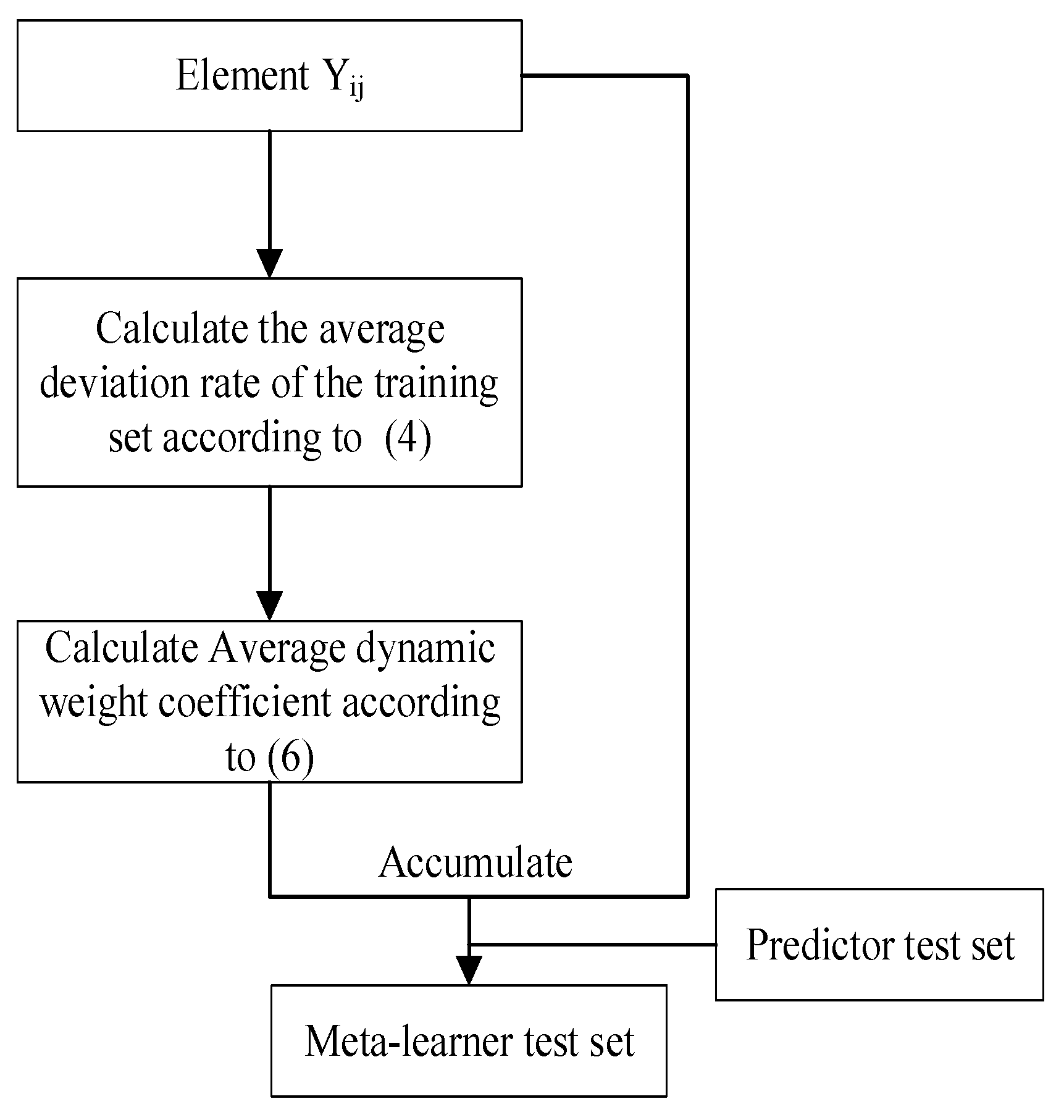
2.4.1. Dynamic Weighting Adjustment Model Process

In the stacking model, the degree of data deviation at different locations in the base learner output information varies, and fixed weighting cannot capture its dynamic change pattern, so dynamic weighting coefficients are designed in the model.

The coefficient is designed outside the meta-learners, and the dynamic weight coefficients are first solved according to the degree of deviation at different positions, and then the dynamic weight coefficients are weighted to adjust the base learner output information to achieve the extraction of dynamic change patterns. The weighting coefficients here include error weighting and entropy weighting.

$Y_{ij}\left(i=1,2,\cdots ,m;j=1,2,\cdots ,n\right)$ is the predicted value of the base learner, $L_i\left(i=1,2,\cdots ,m\right)$ is the actual value, $m$ is the number of elements, $n$ is the number of base learners, and $u_j$ is the predicted mean value of each base learner. The adjustment process of the output information of the base learner is

$${\left(\begin{array}{cccc}{y}_{11}& y_{12}& \cdots & y_{1n}\\ y_{21}& y_{22}& \cdots & y_{2n}\\ \cdots & \cdots & \cdots & \cdots \\ y_{m1}& y_{m2}& \cdots & y_{mn}\end{array}\right)}_{m\times n}\stackrel{transform}{\to }{\left(\begin{array}{cccc}{y}_{11}{x}_{11}& y_{12}{x}_{12}& \cdots & y_{1n}{x}_{1n}\\ y_{21}{x}_{21}& y_{22}{x}_{22}& \cdots & y_{2n}{x}_{2n}\\ \cdots & \cdots & \cdots & \cdots \\ y_{m1}{x}_{m1}& y_{m2}{x}_{m2}& \cdots & y_{mn}{x}_{mn}\end{array}\right)}_{m\times n}\stackrel{prediction}{\to }{\left(\begin{array}{c}{l}_1\\ l_2\\ \cdots \\ l_m\end{array}\right)}_{m\times 1}$$

(11)

In the process of adjustment, the key lies in the solution of dynamic weight coefficients $x_{ij}$.The solution process is as follows:

$$e_{ij}={\left(\begin{array}{cccc}\left|y_{11}-l_1\right|& \left|y_{12}-l_1\right|& \cdots & \left|y_{1n}-l_1\right|\\ \left|y_{21}-l_2\right|& \left|y_{22}-l_2\right|& \cdots & \left|y_{2n}-l_2\right|\\ \cdots & \cdots & \cdots & \cdots \\ \left|y_{m1}-l_{\mathrm{m}}\right|& \left|y_{m2}-l_{\mathrm{m}}\right|& \cdots & \left|y_{mn}-l_{\mathrm{m}}\right|\end{array}\right)}_{m\times n}$$

(12)

(1)

Calculate the absolute error of each element $e_{ij}$, that is, the degree of deviation of each element: the absolute value of the difference between the predicted value $y_{ij}$ and the actual value $l_i$ of the base learner;

$$E_{ij}={\left(\begin{array}{cccc}\frac{\left|y_{11}-l_1\right|-u_1}{u_1{}^{\prime }-u_1}& \frac{\left|y_{12}-l_1\right|-u_2}{u_2{}^{\prime }-u_2}& \cdots & \frac{\left|y_{1n}-l_1\right|-u_n}{u_n{}^{\prime }-u_n}\\ \frac{\left|y_{21}-l_2\right|-u_1}{u_1{}^{\prime }-u_1}& \frac{\left|y_{22}-l_2\right|-u_2}{u_2{}^{\prime }-u_2}& \cdots & \frac{\left|y_{2n}-l_2\right|-u_n}{u_n{}^{\prime }-u_n}\\ \cdots & \cdots & \cdots & \cdots \\ \frac{\left|y_{m1}-l_m\right|-u_1}{u_1{}^{\prime }-u_1}& \frac{\left|y_{m2}-l_m\right|-u_2}{u_2{}^{\prime }-u_2}& \cdots & \frac{\left|y_{mn}-l_m\right|-u_n}{u_n{}^{\prime }-u_n}\end{array}\right)}_{m\times n}$$

(13)

$${\overline{E}}_{ij}={\left(\begin{array}{cccc}\frac{{\displaystyle \sum _{i=1}^m\left|y_{i1}-l_i\right|-m{u}_1}}{m(u_1{}^{\prime }-u_1)}& \frac{{\displaystyle \sum _{i=1}^m\left|y_{i2}-l_i\right|-m{u}_2}}{m(u_2{}^{\prime }-u_2)}& \cdots & \frac{{\displaystyle \sum _{i=1}^m\left|y_{in}-l_i\right|-m{u}_n}}{m(u_n{}^{\prime }-u_n)}\end{array}\right)}_{1\times n}$$

(14)

(2)

Calculate the deviation rate $E_{ij}$ and average deviation rate of each element ${\overline{E}}_{ij}$, the normalized value of absolute error $e_{ij}$, and the normalized mean value of absolute error of each column n $e_{ij}$, respectively;

$$C_{ij}={\left(\begin{array}{cccc}\frac{u_1{}^{\prime }-\left|y_{11}-l_1\right|}{u_1{}^{\prime }-u_1}& \frac{u_2{}^{\prime }-\left|y_{12}-l_1\right|}{u_2{}^{\prime }-u_2}& \cdots & \frac{u_n{}^{\prime }-\left|y_{1n}-l_1\right|}{u_n{}^{\prime }-u_n}\\ \frac{u_1{}^{\prime }-\left|y_{21}-l_2\right|}{u_1{}^{\prime }-u_1}& \frac{u_2{}^{\prime }-\left|y_{22}-l_2\right|}{u_2{}^{\prime }-u_2}& \cdots & \frac{u_n{}^{\prime }-\left|y_{2n}-l_2\right|}{u_n{}^{\prime }-u_n}\\ \cdots & \cdots & \cdots & \cdots \\ \frac{u_1{}^{\prime }-\left|y_{m1}-l_m\right|}{u_1{}^{\prime }-u_1}& \frac{u_2{}^{\prime }-\left|y_{m2}-l_m\right|}{u_2{}^{\prime }-u_2}& \cdots & \frac{u_n{}^{\prime }-\left|y_{mn}-l_m\right|}{u_n{}^{\prime }-u_n}\end{array}\right)}_{m\times n}$$

(15)

$${\overline{C}}_{ij}={\left(\begin{array}{cccc}\frac{m{u^{\prime }}_1-{\displaystyle \sum _{i=1}^m\left|y_{i1}-l_i\right|}}{m(u_1{}^{\prime }-u_1)}& \frac{m{u^{\prime }}_2-{\displaystyle \sum _{i=1}^m\left|y_{i2}-l_i\right|}}{m(u_2{}^{\prime }-u_2)}& \cdots & \frac{m{u^{\prime }}_n-{\displaystyle \sum _{i=1}^m\left|y_{in}-l_i\right|}}{m(u_n{}^{\prime }-u_n)}\end{array}\right)}_{1\times n}$$

(16)

(3)

Calculate the contribution rate $C_{ij}$ and the average contribution rate of each element ${\overline{C}}_{ij}$, the value of 1 minus the deviation rate, and the value of 1 minus the average deviation rate, respectively.

The contribution rate calculated in Equation (14) is the dynamic weight coefficient $C_{ij}$. The adjusted output information reduces the prediction results influenced by errors or deviation information, making the information characteristics more representative. The coefficient matrices are used to adjust the training set and test set. The specific process is as follows:

• Training set

Adjust the change rule of the predicted value of the base learner: use the product of the predicted value of different positions and the dynamic weight coefficient as the new data. The specific process is shown in Figure 5.

• Test set

Adjust the overall change law of the predicted value of the training set of the base learner: use the product of the predicted value of different positions and the average dynamic weight coefficient in the training set as the new data. The specific process is shown in Figure 6.

2.4.2. Ba-Stacking Model Optimization Process

The principle of the improved stacking ensemble model is shown in Figure 7. Assuming that the traffic flow data sequence has $X$ records of data, $N$ is the number of characteristic variables, the original data set is $\left\{\left(Y_{0X}, Q_{iX}\right)\right\}$, $Y_{0X}\left(X=1,2,\dots ,N\right)$ is the predictor variable, and $Q_{iX}$ is the characteristic variable. The specific steps of the model are as follows:

(1)

Divide the original data into the training set and test set;

(2)

Construct the corresponding prediction models, including random forest, XGBoost, the GBDT, and the decision-tree model;

(3)

Use $Q_{iX}$ and $Y_{0X}$ to obtain the corresponding predicted values of different models through the bagging algorithm, denoted as $Y_{1X},Y_{2X},Y_{3X},Y_{4X},Y_{5X},Y_{6X}$;

(4)

Using $Y_{1X},Y_{2X},Y_{3X},Y_{4X},Y_{5X},Y_{0X}$, obtain the weight coefficients by different adjustment methods, followed by the flow data of the adjusted base learner model, noted as $Y_{1X}^{\prime },Y_{2X}^{\prime },Y_{3X}^{\prime },Y_{4X}^{\prime },Y_{5X}^{\prime }$;

(5)

Using$Y_{1X}^{\prime },Y_{2X}^{\prime },Y_{3X}^{\prime },Y_{4X}^{\prime },Y_{5X}^{\prime }$,$Y_{0X}$, build a meta-learner ridge regression mode to obtain the final traffic prediction values of the improved stacking integration model;

(6)

Train the model with the training set. Once trained, the model will be tested using the test set.

3. Problem Description and Data Progress

3.1. Overview of Short-Term Traffic Flows

Traffic flow is the volume of traffic formed by vehicles on a roadway. The factors influencing traffic flow include flow, speed, and occupancy. Traffic flow is an important indicator to determine traffic congestion, its prediction results are an important parameter to grasp the city traffic situation, and the selection of the prediction time period is an important step in the prediction process. There are various types of traffic flow data recorded by monitoring point detectors, including 30s, 5 min, 15 min, 30 min, and 60 min, depending on the collection time, and highways and urban roads depending on the type of road collected. Traffic-flow prediction results are usually obtained from the historical data function, that is, the historical information within the time of $\left(t_{i-j},t_{i-1}\right)$ predicts the current information of $t_i$.

$$t_i=f\left(t_{i-j}\right)$$

(17)

$t_i$ stands for the current time of the indicator value$t_{i-j}$ stands for the historical time period of the indicator value, and the function indicates the historical time period of the traffic value to predict the future time period of the traffic value. When the adjacent time interval $\Delta t$ is less than or equal to 15 min, the formula represents the short time traffic flow forecast, so this paper chooses 15 min as the time interval for traffic-flow prediction and analysis.

In short-term traffic-flow forecasting, occupancy and speed are the important impact indicators of road traffic; this paper will focus on the two indicators as the flow of the constraint characteristics, and its historical trend to join the traffic-flow forecasting; the function relationship is shown as follows:

$$l_i=f\left(z_{i-j},v_{i-j},l_{i-j}\right)$$

(18)

$z_{i-j},v_{i-j},l_{i-j}$ refers to the values of occupancy, speed, and traffic flow indicators, respectively, at the historical moment;$i$ is the current time; and$j$ is the historical time period used.$j$ = 4 is chosen for the prediction analysis in this paper.

3.2. Data Sources and Pre-Processing

3.2.1. Data Sources

The data selected for this paper is from the PORTAL dataset, which provides official traffic data for Portland, USA and Vancouver, Canada, with monitors recording traffic at five intervals: 30 s, 5 min, 15 min, 30 min, and 60 min. Traffic data for 15 min intervals on the I5NB highway in Portland, USA are selected for analysis, and the main data tables studied are the monitor data tables.

The data set occupancy and speed are data features that can be directly utilized in the data tables. These two indicators are also the actual indicators that affect the traffic flow, so these two indicators are used as input features to the model. The timestamp feature is the time recorded by the detector, which can provide some regular reference for the trend change of the traffic flow; the specific feature construction analysis is in Section 3.2.3, so this indicator is also used as an input feature, and the traffic flow is input into the model as an output feature for prediction. The data analyzed for the example in this paper is 100703 detector data, collected at the specific time of 1 February 2018 00:00:00–12 April 2020 0:00:00, with 96 data per day, comprising a total of 76,896 pieces of data. Seventy percent of the data set was used as the training set and 30% of the data set was used as the test set.

3.2.2. Feature Construction

According to the analysis in Section 3.1, occupancy and speed can effectively influence traffic flows, so these two indicators are entered into the forecasting model as intrinsic characteristics. In addition to the intrinsic characteristics, the trend of traffic flow can be influenced by certain external characteristics that can affect the accuracy of the forecast, especially the temporal characteristics: traffic flow has obvious cyclical characteristics, so the cyclical temporal characteristics are important characteristics affecting the traffic flow; for example, there is more traffic flow during peak hours or holidays, so the extraction of the temporal characteristics plays an important role. To explore the temporal characteristics of traffic flow in depth, the trend of traffic flow changes over a period of time is randomly selected for analysis, as shown in Figure 8.

It can be seen that the same characteristics of variation occur each day, and it is obvious that there are two peaks, the peak commuting period and the peak leaving period, which are in line with the characteristics of real-life variation. This work makes full use of the historical data of the traffic flow and adds the relevant historical data of occupancy and speed as features to the prediction of the model as well. The specific construction process is as follows.

(1)

Structured rest day features

Holidays and weekends are days off, and people can choose to stay at home or travel depending on the situation; therefore, the traffic flow situation is different between rest days and weekdays, so this feature is used as an important feature for predicting traffic flow. This work extracts holiday data and weekday data from the temporal features of the traffic flow collection.

(2)

Construction work peak characteristics

The peak information is also used as an important indicator for predicting traffic flow, considering people’s daily life habits, i.e., there will be normal commuting in the morning and evening, so there is more traffic flow at this time, which will also affect the prediction results. In this paper, 6:00–8:00 am and 17:00–19:00 pm are taken as the peak time periods. If this time is the peak hour, it is set to 1; otherwise, it is set to 0.

(3)

Constructing historical indicator characteristics

Speed is the distance travelled by vehicles per unit of time, and occupancy is time occupancy and space occupancy, respectively, indicating the density of vehicles; these two indicators have a strong correlation with traffic flow, and this paper sets the sliding window to 4, i.e., occupancy and speed in 4 time periods as historical indicator features, aiming to extend the feature structure of the traffic-flow prediction model and improve the overall performance of the model.

(4)

One-hot encoding processing

One-hot encoding, also known as one-hot encoding or one-valid encoding, is a method of encoding N states using N-bit state registers, each of which has its own register and only one of which is valid at any given time. The method uses N-bit status registers to encode N states, each of which has its own independent register bits and only one of which is valid at any given time. One-hot is a method for processing discrete data and converting different discrete data into continuous data, and this paper uses this method to convert temporal features into continuous temporal features.

Occupancy, speed, and traffic flow are all features of the original data table, while holidays, weekends, and peaks are expanded features of the original data table and are discrete data features. Therefore, this paper uses one-hot to process this discrete data and uses this data and the historical occupancy, speed, and traffic flow as features to input into the model. The time features are interpreted in detail as follows: a holiday feature of 0 means this time is not a holiday; a weekend feature of 1 means the time is a weekend; and a peak information feature of 0 means this time is not a peak time period.

3.2.3. Data Pre-Processing

In the process of traffic flow detection, the recorder of the detection data may be affected by some random factors to produce missing data, such as weather and climate, road driving conditions, the recorder itself, etc., and these data are important parts of the model prediction. The way the data are processed plays a key role in the accuracy of the prediction, so it is necessary to effectively deal with the missing part of the data. The difference in the data size will also cause an error in the prediction, and as the data size required for each monitoring point is different, some processing needs to be done to eliminate the error.

Missing Value Handling

There are two types of data loss: the first is the loss of an entire record, which can be caused by the failure of a logger, but this is uncommon; the second is the loss of part of a record, where a value is not recorded during the monitoring of the logger for reasons external to the logger, and thus part of the data is missing.

The traffic flow data in this paper have a low missing rate, and for the continuous variation characteristic of the missing values, this paper uses mean filling, specifically with the mean of the last five values of the same time attribute in history.

Data Normalization

Data normalization is an important step in data processing, where a certain amount of data is scaled down to a certain range so that the input features of the model vary within a smaller range, thereby eliminating the error generated in the model by the variability of the feature magnitudes. In this paper, we use the maximum-minimum normalization method to vary the original data features to within [0, 1], as a function of

$$x^{\prime }=\frac{x-min}{max-min}$$

(19)

where $min$ is the minimum value of each feature and $max$ is the maximum value of each feature; the larger the value of the metric in each feature, the closer to 1 it will be after the change.

4. Experiment

4.1. Evaluation Indicators

This work selects the mean squared error (MSE) and mean absolute error (MAE) to evaluate the prediction effect of each model. The formula is shown as follows:

$$MSE=\frac{1}{n}{\displaystyle \sum }_{i=1}^n{\left[Y\prime \left(i\right)-Y\left(i\right)\right]}^2$$

(20)

$$MAE=\frac{1}{n}{\displaystyle \sum }_{i=1}^n\left|Y\prime \left(i\right)-Y\left(i\right)\right|$$

(21)

where $Y\prime \left(i\right)$ is the predictor variable, $Y\left(i\right)$ is the actual variable, and $n$ is the number of records of the data.

4.2. Model Prediction

In order to verify the effectiveness of the algorithm, this paper adds a comparative analysis with other models, including single models such as random forest, GBDT, other single models before and after feature optimization, stacking ensemble models before and after improvements, and other combined models.

4.2.1. Analysis of Feature Prediction Effect

In this paper, considering the correlation between historical data and future data, the first four periods of the time data of the occupancy rate and the speed are added to the characteristics of the model. In the actual model prediction, the addition of features has a more obvious optimization effect on the random forest. In order to analyze the effects of historical related characteristics, some single models such as XGBoost, DBDT, and decision tree are selected for comparative analysis, shown as

Table 1. A comparative analysis of the prediction effects of different characteristics.

Base Learner	Historical Characteristics	Time Characteristics	MSE	MAE
Random forest	+	+	662.11	17.38
	+	-	745.40	18.08
	-	-	761.44	18.26
XGBoost	+	+	649.15	17.27
	+	-	762.76	18.40
	-	-	773.18	18.40
GBDT	+	+	648.21	17.25
	+	-	760.87	18.32
	-	-	778.18	18.44
Decision tree	+	+	754.31	18.45
	+	-	778.73	18.70
	-	-	789.33	18.81
KNN	+	+	754.37	18.63
	+	-	776.90	18.36
	-	-	789.40	18.50
GRU	+	-	744.73	18.54
	-	-	768.01	18.72

Note: + having this characteristic; - not having this characteristic.

.

It can be clearly seen from Table 1 that the selection of features has improved the overall model prediction performance. From the perspective of MSE and MAE, for all models, the structure of time features has different degrees of improvement for different models and determines whether the deep learning or the representative machine learning model is used. The more obvious are the GBDT model and the random forest model of the integrated tree model. The MSE has been improved by more than 20, followed by the XGBoost model and the GRU model, and the last is a relatively single KNN model and the decision-tree model. This conclusion shows that the single model is not as sensitive as the integrated mode.

For learners other than deep learning, after adding historical features and time features, each machine learning model experiences a greater degree of improvement: the accuracy of a single model is limited and the improved MSE is within 50. For the integrated model, the addition of this feature makes a greater contribution to the improvement: the MSE’s improvement space is about 100, of which the boosting integrated model constitutes the largest improvement and the GBDT accuracy improvement is the largest, followed by XGBoost. Therefore, from the analysis of the fusion of the two features, it can be analyzed that the integrated model is more sensitive to the model features.

In order to analyze part of the effect of model prediction, add Figure 9, Figure 10 and Figure 11 for a more detailed analysis, i.e., to select one day’s traffic flow data for analysis randomly, with the aim to analyze the prediction effects of different characteristics. It can be seen from the figure that the change trend of different models after adding features is roughly the same, and the prediction effect is better than that without adding features. The more features are integrated, the closer the prediction curve is to the original data line.

4.2.2. Single Model Parameter Setting

The grid search is a method of adjusting parameters. First, set a set of candidate values for the parameters you want to adjust, and then the grid search will exhaust various parameter combinations and find the best set of settings according to the set scoring mechanism. In the actual machine model, there are many parameters, so it is impossible to manually adjust the parameters in a timely and effective manner. Therefore, the parameters of different learning models can be automatically adjusted through the grid search method to obtain the parameters with the highest prediction accuracy. In this paper, the grid search is applied to the base learner, with the aim to find the parameter features when the accuracy is optimal.

In the model building process, other variables in the data table except the volume variable are used as the input variables, and the volume variable is used as the dependent variable to construct the following single predictive model. Among them, random forest, XGBoost, GBDT, KNN, and the decision tree use the network search method to adjust the parameters, and the GRU model adopts manual parameter adjustment. The parameter settings of each single model and the error after parameter adjustment are shown in

Table 2. The single model prediction.

Base Learner	Parameter Setting	MSE	MAE
Random forest	The tree depth is 10, the number of trees is 160, the minimum number of samples for leaf nodes is 2, and the minimum number of samples for the node division is 5	662.11	17.38
XGBoost	The number of trees is 390, the minimum leaf node sample weight is 8, the random sampling ratio is 0.9, the number of columns randomly sampled in each tree accounts for 0.8, and the learning rate is 0.12	649.15	17.27
GBDT	The tree depth is 3, the number of trees is 470, the minimum number of samples for leaf nodes is 6, and the minimum number of samples for node division is 10	648.21	17.25
KNN	Take the number of adjacent points: 48	754.37	18.63
Decision tree	The tree depth is 7, the minimum number of samples for leaf nodes is 2, and the minimum number of samples for node division is 7	754.31	18.45
GRU	GRU has two layers of neurons, of which the number in the first layer is 64 and that in the second layer is 32. The dropout is 0.1	744.73	18.54

. The prediction effects of different models are shown in the Figure 12.

It can be seen that among many models, the integrated model performs well in this traffic-flow prediction. The GBDT model performs best, followed by the bagging algorithm, represented by random forest model. The deep-learning model GRU performs moderately well. The single-model KNN and decision tree perform poorly. It can be seen that, compared to the single model, the integrated model is more suitable for traffic-flow prediction, and the boosting integrated tree model performs better.

Figure 12 shows an error map of selected different models in a day. It can be seen that the error variation characteristics of six single models are the same. Among them, the fluctuation error of the KNN model and the decision-tree model is larger; the error fluctuation of the other models are smaller, indicating that the prediction stability of these four models is better. From Table 2, it can be seen that the prediction effects of the six models are distributed in two sets, of which GBDT has the best prediction effect, and its MSE is 648.21, which is 7.8% less than the MSE of KNN, with a larger error, while the prediction effect of Random forest, GDBT, and XGBoost is better. Therefore, from the perspective of overall or partial predictive analysis results, the stability and accuracy of integrated model prediction are higher than that of a single model.

4.2.3. Pearson Characteristic Coefficient Analysis

The coefficients that measure the degree of correlation between variables include the Pearson correlation coefficient, the Spearman’s correlation coefficient, and Kendall’s correlation coefficient. Among them, the Pearson correlation coefficient can represent the linear coefficient value between variables. In recent years, it has been used by major models to screen the features of competitions, and it has good applicability. In the overall architecture of the stacking model, the output information of the base learner model is used as the important feature information of the prediction information, and the degree of its association with the prediction information affects the final prediction result. In this paper, the Pearson correlation coefficient is used to measure the correlation and screening process between the output information and prediction information of the base learner model. The coefficients obtained are shown in the

Table 3. The Pearson coefficient analysis table.

	R	X	GB	D	K	G	Y
R	1	0.9962	0.9964	0.9890	0.9932	0.9895	0.9441
X	0.9962	1	0.9988	0.9869	0.9898	0.9891	0.9444
GB	0.9964	0.9988	1	0.9870	0.9900	0.9891	0.9442
D	0.9890	0.9869	0.9870	1	0.9829	0.9849	0.9354
K	0.9932	0.9898	0.9901	0.9829	1	0.9877	0.9355
G	0.9895	0.9891	0.989123	0.9849	0.9877	1	0.9357
Y	0.9441	0.9444	0.9442	0.9354	0.9354	0.9357	1

Note: R is the random forest model, X is the XGBoost model, GB is the GBDT model, D is the decision-tree model, K is the KNN model, G is the GRU model, and Y is the actual traffic flow variable.

.

In Table 3, the fourth column is the correlation degree between the features of the corresponding base learner and the predictor variables. The closer it is to 1, the greater the correlation. The correlation coefficients of all base learner variables and predictor variables are bigger than 0.9, indicating that the degree of correlation is greater, and its use effect will affect the final result. Under the premise that the base model is known, knowing how to choose an effective model plays a key role in the accuracy of the prediction results. Next, the selection of the model is analyzed in detail.

In order to analyze the effects of different base learners in the stacking model, this paper takes the ridge regression meta-learner as an example to establish the final prediction effect under different base learner combinations. The prediction results are shown in

Table 4. The model selection analysis table.

Model Selection	Y/N	Y/N	Y/N	Y/N	Y/N	Y/N
Random forest	1	1	1	1	1	1
GBDT	1	1	0	1	1	1
XGBoost	1	0	1	1	1	1
KNN	1	1	0	0	0	0
Decision tree	1	1	1	0	1	0
GRU	1	1	1	1	1	1
MSE	638.15	638.92	638.71	643.67	638.63	643.01
MAE	17.07	17.06	17.07	17.17	17.08	17.15

Note: This applies to situations in which yes is 1; in other situations, it is 0.

.

The base learner in the stacking model selected in this paper has different characteristics, and knowing how to combine effective models has a greater impact on the final result. The above table is the MSE and MAE index values that combine different models. It can be seen that the smallest values of MSE and MAE indicators are achieved when the six models are combined. From Table 3, it can be seen that the correlation coefficient of each model is greater than 0.92, so the output information of the model-based learner and the actual information have a great correlation. After removing the models with small or large correlations, their accuracy is reduced to varying degrees. Therefore, the stacking model requires a certain degree of difference. When the integrated model represents all models with better base learner accuracy, its accuracy is not the highest, and after removing part of the model information in this table, its accuracy is reduced. Therefore, the stacking-integrated model of the six machine models proposed in this paper can make predictions more effectively.

4.2.4. Ba-Stacking Model Prediction

In order to analyze the improvement effect of the bagging algorithm integrated with different base learner models on the stacking integration algorithm, the Ba-Stacking model of different base learner models is established, and the final MSE and MAE are used to specifically evaluate the prediction effect, as shown in

Table 5. The Ba-Stacking model prediction effect of different meta-learners.

Meta-Learner	Bagging					Evaluation Index
	Random Forest	XGBoost	GBDT	Decision Tree	KNN	MSE	MAE
Ridge regression	-	-	-	-	-	638.15	17.07
	+	-	-	-	-	641.15	17.11
	-	+	-	-	-	637.33	17.06
	-	-	+	-	-	637.51	17.06
	-	-	-	+	-	638.14	17.07
	-	-	-	-	+	633.83	17.00
	+	+	+	+	+	634.95	17.00
	-	+	+	+	+	632.85	16.99

Note: + using this model; - not using this model

.

It can be seen from Table 5 that the prediction accuracy of the overall stacking model has decreased after the integration of the random forest optimized by bagging. The integration of other machine learning models optimized by bagging has improved the overall stacking model. The random forest model optimized by the bagging algorithm is not as good as the original random forest model, which affects the performance of the ensemble model. After bagging with the integration of other optimized models, the prediction accuracy of the stacking ensemble model has been improved compared to the original stacking ensemble model, and the base learner model that has been optimized by the bagging algorithm is integrated, namely, the optimized XGBoost, GBDT, decision-tree, and the stacking-integrated models after the KNN-based learner model make more accurate predictions. Therefore, whether from the horizontal or vertical angle of the table, it can be seen that the accuracy of the stacking model optimized by the bagging algorithm has improved the accuracy of the original model to varying degrees. We can know that this method optimizes the overall performance under the premise of optimizing the base learner.

4.2.5. DW-Ba-Stacking Model Prediction

In order to verify the effectiveness of this model, take the mentioned optimal single model prediction result as input and actual traffic flow as output; ridge regression is established as the original stacking ensemble model and the DW-Ba-Stacking model of the meta-learner. The prediction effect of each single model and each combination model is shown in

Table 6. A performance analysis of each combination model.

Method	MSE	MAE
Random forest	662.11	17.38
XGBoost	649.15	17.27
GBDT	648.21	17.25
KNN	754.37	18.63
Decision tree	754.31	18.45
GRU	744.73	18.54
Stacking model	638.15	17.07
Ba-Stacking model	632.85	16.99
DW-Ba-Stacking model	619.59	16.87
Reciprocal error method combination	659.31	17.28

, and the prediction effect is shown in the Figure 13.

Table 6 shows the prediction results of different combination models. From the prediction results, it can be seen that the prediction effect of other combination models is poor. Because there are many single models in this paper, the advantages of the single models cannot be well integrated; the stacking ensemble model has better prediction results than other combination models, among which is stacking. The base learners of the ensemble model are XGBoost, GBDT, decision tree, random forest, and GRU. The stacking model, whose meta-learner is ridge regression, is weighted by entropy; the MSE of the original model is reduced; and the MAE index value is reduced. The improved stacking model after error weighting is less than the MSE of the original model, and the MAE index value is reduced. Compared with the improved stacking ensemble model of the GRU meta-learner, the improved effect of the meta-learner is the ridge regression; obviously, it can be seen that the stacking ensemble models improved by different weights have optimization effects, and the stacking ensemble model of error-weighted ridge regression has the best optimization effect.

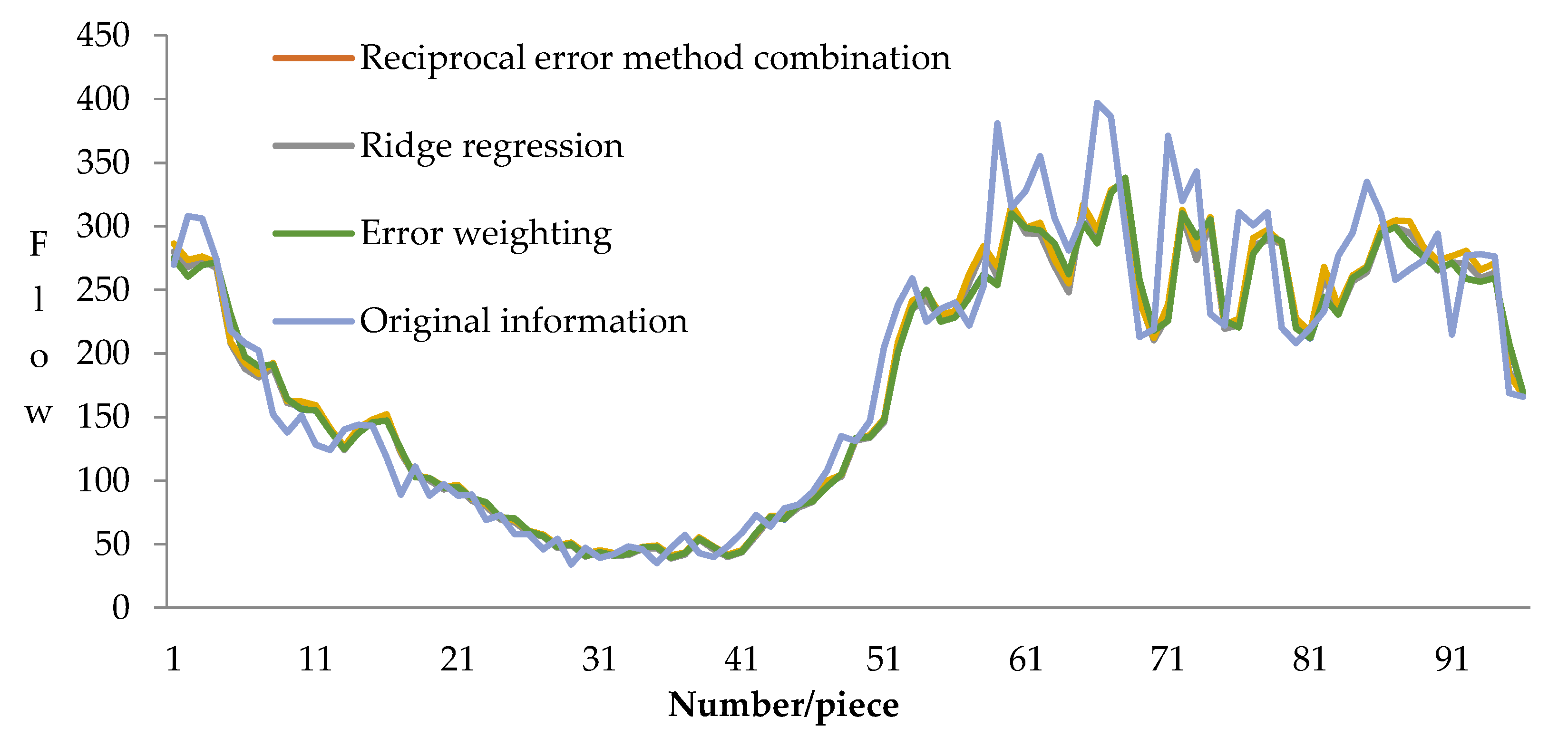
4.2.6. Comparative Analysis of Experimental Results

The model comparison analysis includes the basic learner model under different characteristics in the literature [9,10,11,12,15], the Ba-Stacking model optimized by the bagging algorithm, and the DW-Ba-Stacking model; the prediction results analysis as shown in the

Table 7. The comparison table of different models.

Models		MSE	MAE
Single model	Random forest [9]	706.68	18.72
	XGBoost [10]	694.99	18.54
	GBRT [11]	691.63	18.51
	KNN [12]	830.83	20.40
	GRU [15]	773.54	19.89
Meta-learner for ridge regression	Stacking	689.79	18.46
	Ba-Stacking	688.35	18.45
	DW-Ba-Stacking	681.39	18.22

. The comparative analysis further verifies that the model proposed in this paper has higher prediction accuracy and stronger applicability.

5. Conclusions

With socio-economic improvements, traffic congestion will occur more frequently. Traffic-flow prediction can effectively manage and monitor traffic flow, and its prediction accuracy plays a crucial role in solving traffic-congestion problems. Machine learning algorithms have long been applied to the field of traffic-flow prediction, but individual models are greatly limited in terms of their predictive powers. Therefore, this paper applies the stacking-integrated learning model, which has been widely used in various fields in recent years, to traffic-flow prediction and provides a new idea for its prediction. A series of improvement measures are carried out to address the shortcomings of the traditional stacking-integrated learning model. The main objectives of this paper are as follows:

(1)

In order to improve the shortcomings of the traffic prediction model with a single feature, temporal features such as holidays and historical features such as speed are constructed. Traffic flow is always recorded in the detector, so the time for the recorded parameters is clearer. In this paper, different time-feature information is extracted according to the specific time of the record: holiday information, weekend information features, and peak information; historical speed and occupancy features related to traffic flow are constructed according to the original data features, and the rationality of the introduced features is verified through the comparative analysis of different features. Thus, the best effect is obtained.

(2)

The stacking integration model with the highest accuracy is obtained by filtering and optimizing the learners. First, we build machine learning models with different merits; then, we analyze the correlation coefficient between each model and the actual information by using the Pearson correlation coefficient; next, we select the stacking-integrated model with the highest prediction accuracy based on the weight of each model; and, finally, we embed the bagging model in this model to further improve the prediction accuracy of the model.

(3)

According to the shortcomings of the stacking-integrated model, the stacking model two-layer is used as the object of improvement. With the goal of enhancing the variability between models and the correlation between predicted and actual information, the weights of different base learner models are adjusted so that the prediction accuracy is higher.

The main innovative work of this paper is to achieve the following:

(1)

Realize the effective combination of the stacking model and bagging model, i.e., the construction of Ba-Stacking. The bagging model is used to optimize the output information features of the base learner in the stacking model, and the construction of the Ba-Stacking model is completed.

(2)

Based on the Ba-Stacking model, the DW-Ba-Stacking model is constructed by weighting coefficients. The Ba-Stacking model with the meta-learners as ridge regression optimizes the base learner feature information by error coefficient.

In summary, this paper not only introduces the stacking-integrated model, which can effectively improve the accuracy of traffic-flow prediction, but also proposes an improved DW-Ba-Stacking model, which further improves the prediction accuracy of traffic flow while adjusting the internal structure, and provides a reference for the development of traffic-management strategies and implementation plans. In the future, the improved method can be applied to other fields with practical significance. However, in the process of improving the stacking ensemble model, this paper only pays attention to the prediction accuracy and does not consider the time efficiency, so there are some limitations in its level of improvement. In the future, the improved method can be applied to other fields with practical significance.

References

1. Alghamdi, T.; Elgazzar, K.; Bayoumi, M.; Sharaf, T.; Shah, S. Forecasting Traffic Congestion Using ARIMA Modeling. In Proceedings of the 2019 15th International Wireless Communications & Mobile Computing Conference (IWCMC), Tangier, Morocco, 24–28 June 2019; pp. 1227–1232. [Google Scholar]
2. Min, X.; Hu, J.; Zhang, Z. Urban traffic network modeling and short-term traffic flow forecasting based on GSTARIMA model. In Proceedings of the 13th International IEEE Conference on Intelligent Transportation Systems, Funchal, Portugal, 19–22 September 2010; pp. 1535–1540. [Google Scholar]
3. Liu, X.W. Research on Highway Traffic Flow Prediction and Comparison based on ARIMA and Long-Short-Term Memory Neural Network. Master’s Thesis, Southwest Jiaotong University, Chengdu, China, 2018. (In Chinese). [Google Scholar]
4. Cvetek, D.; Muštra, M.; Jelušić, N.; Abramović, B. Traffic Flow Forecasting at Micro-Locations in Urban Network using Bluetooth Detector. In Proceedings of the 2020 International Symposium ELMAR, Zadar, Croatia, 14–15 September 2020; pp. 57–60. [Google Scholar]
5. Iwao, J.; Stepphanedes Yorgos, J. Dynamic prediction of traffic volume through Kalman filtering theory. Pergamon 1984, 18, 1–11. [Google Scholar]
6. Guo, J.; Huang, W.; Williams, B.M. Adaptive Kalman filter approach for stochastic short-term traffic flow rate prediction and uncertainty quantification. Transp. Res. Part C Emerg. Technol. 2014, 43, 50–64. [Google Scholar] [CrossRef]
7. Ullah, I.; Fayaz, M.; Naveed, N.; Kim, D. ANN Based Learning to Kalman Filter Algorithm for Indoor Environment Prediction in Smart Greenhouse. IEEE Access 2020, 8, 159371–159388. [Google Scholar] [CrossRef]
8. Vlahogianni, E.I.; Karlaftis, M.G.; Golias, J.C. Short-term traffic forecasting: Where we are and where we’re going. Transp. Res. Part C Emerg. Technol. 2014, 43, 3–19. [Google Scholar] [CrossRef]
9. Gao, J.; Leng, Z.; Qin, Y.; Ma, Z.; Liu, X. Short-term traffic flow forecasting model based on wavelet neural network. In Proceedings of the Control and Decision Conference (CCDC), Guiyang, China, 25–27 May 2013; pp. 5081–5084. [Google Scholar]
10. Qin, Y.; Adams, S.; Yuen, C. Transfer Learning-Based State of Charge Estimation for Lithium-Ion Battery at Varying Ambient Temperatures. IEEE Trans. Ind. Inform. 2021, 17, 7304–7315. [Google Scholar] [CrossRef]
11. Xiong, T.; Qi, Y.; Zhang, W.B.; Li, Q.M. Short-term traffic flow prediction model based on spatiotemporal correlation. Comput. Eng. Des. 2019, 40, 501–507. (In Chinese) [Google Scholar]
12. Lu, W.; Rui, Y.; Yi, Z.; Ran, B.; Gu, Y.A. Hybrid Model for Lane-Level Traffic Flow Forecasting Based on Complete Ensemble Empirical Mode Decomposition and Extreme Gradient Boosting. IEEE Access 2020, 8, 42042–42054. [Google Scholar] [CrossRef]
13. Alajali, W.; Zhou, W.; Wen, S.; Wang, Y. Intersection Traffic Prediction Using Decision Tree Models. Symmetry 2018, 10, 386. [Google Scholar] [CrossRef] [Green Version]
14. Yu, S.; Li, Y.; Sheng, G.; Lv, J. Research on Short-Term Traffic Flow Forecasting Based on KNN and Discrete Event Simulation. In Proceedings of the 15th International Conference on Advanced Data Mining and Applications, Foshan, China, 12–15 November 2019; pp. 853–862. [Google Scholar]
15. Qin, Y.; Yuen, S.C.; Qin, M.B.; Li, X.L. Slow-varying Dynamics Assisted Temporal Capsule Network for Machinery Remaining Useful Life Estimation. arXiv 2022, arXiv:2203.16373. [Google Scholar] [CrossRef] [PubMed]
16. Dai, G.W.; Ma, C.X.; Xu, X.C. Short-Term Traffic Flow Prediction Method for Urban Road Sections Based on Space Time Analysis and GRU. IEEE Access 2019, 7, 143025–143035. [Google Scholar]
17. Hu, H.; Yan, W.; Li, H.M. Short-term traffic flow prediction of urban roads based on combined forecasting method. Ind. Eng. Manag. 2019, 24, 107–115. [Google Scholar]
18. Zhu, P.F.; Liu, Y. Prediction of distributed optical fiber monitoring data based on GRU-BP. In Proceedings of the 2021 International Conference on Intelligent Transportation, Big Data & Smart City (ICITBS), Xi’an, China, 27–28 March 2021; pp. 222–224. [Google Scholar]
19. Barboza, F.; Kimura, H.; Altman, E. Machine learning models and bankruptcy prediction. Expert Syst. Appl. 2017, 83, 405–417. [Google Scholar] [CrossRef]
20. Wang, S.; Yao, Y.; Xiao, Y.; Chen, H. Dynamic Resource Prediction in Cloud Computing for Complex System Simulatiuon: A Probabilistic Approach Using Stacking Ensemble Learning. In Proceedings of the 2020 International Conference on Intelligent Computing and Human-Computer Interaction (ICHCI), Sanya, China, 4–6 December 2020; pp. 198–201. [Google Scholar]
21. Liu, Y.; Yang, C.; Gao, Z.; Yao, Y. Ensemble deep kernel learning with application to quality prediction in industrial polymerization processes. Chemom. Intell. Lab. Syst. 2018, 174, 15–21. [Google Scholar] [CrossRef]
22. Zhang, X.M.; Wang, Z.J.; Liang, L.P. A Stacking Algorithm for Convolutional Neural Networks. Comput. Eng. 2018, 44, 243–247. [Google Scholar]
23. Li, B.S.; Zhao, H.Y.; Chen, Q.K.; Cao, J. Prediction of remaining execution time of process based on Stacking strategy. Small Microcomput. Syst. 2019, 40, 2481–2486. (In Chinese) [Google Scholar]
24. Sun, X.J.; Lu, X.X.; Liu, S.F. Research on combined traffic flow forecasting model based on entropy weight method. J. Shandong Univ. Sci. Technol. (Nat. Sci. Ed.) 2018, 37, 111–117. (In Chinese) [Google Scholar]
25. Gong, Z.H.; Wang, J.N.; Su, C. A weighted deep forest algorithm. Comput. Appl. Softw. 2019, 36, 274–278. (In Chinese) [Google Scholar]
26. Zheng, Z.H.; Huang, M.F. Traffic Flow Forecast Through Time Series Analysis Based on Deep Learning. IEEE Access 2020, 8, 82562–82570. [Google Scholar] [CrossRef]
27. Zhao, Z.; Chen, W.; Wu, X.; Chen, P.C.; Liu, J. LSTM network: A deep learning approach for short-term traffic forecast. IET Intell. Transp. Syst. 2017, 11, 68–75. [Google Scholar] [CrossRef] [Green Version]
28. Li, Y.L.; Tang, D.H.; Jiang, G.Y.; Xiao, Z.T.; Geng, L.; Zhang, F.; Wu, J. Residual LSTM Short-Term Traffic Flow Prediction Based on Dimension Weighting. Comput. Eng. 2019, 45, 1–5. (In Chinese) [Google Scholar]
Figure 1. The KNN schematic diagram.
Electronics 11 01467 g001
Figure 2. The decision tree model.
Electronics 11 01467 g002
Figure 3. The GRU structure diagram.
Electronics 11 01467 g003
Figure 4. The Ba-Stacking model architecture diagram.
Electronics 11 01467 g004
Figure 5. The meta learner training set adjustment process.
Electronics 11 01467 g005
Figure 6. The meta learner test set adjustment process.
Electronics 11 01467 g006
Figure 7. The DW-Ba-Stacking model principle diagram (ridge regression).
Electronics 11 01467 g007
Figure 8. The traffic flow trend.
Electronics 11 01467 g008
Figure 9. The GBDT feature-analysis diagram.
Electronics 11 01467 g009
Figure 10. The decision tree feature-analysis diagram.
Electronics 11 01467 g010
Figure 11. The GRU feature-analysis diagram.
Electronics 11 01467 g011
Figure 12. The error graphs of different models.
Electronics 11 01467 g012
Figure 13. The single model error diagram.
Electronics 11 01467 g013