Abstract
Interest in delivering cellular communication using a high-altitude platform (HAP) is increasing partly due to its wide coverage capability. In this paper, we formulate analytical expressions for estimating the area of a HAP beam footprint, average per-user capacity per cell, average spectral efficiency (SE) and average area spectral efficiency (ASE), which are relevant for radio network planning, especially within the context of HAP extended contiguous cellular coverage and capacity. To understand the practical implications, we propose an enhanced and validated recursive HAP antenna beam-pointing algorithm, which forms HAP cells over an extended service area while considering beam broadening and the degree of overlap between neighbouring beams. The performance of the extended contiguous cellular structure resulting from the algorithm is compared with other alternative schemes using the carrier-to-noise ratio (CNR) and carrier-to-interference-plus-noise ratio (CINR). Results show that there is a steep reduction in average ASE at the edge of coverage. The achievable coverage is limited by the minimum acceptable average ASE at the edge, among other factors. In addition, the results highlight that efficient beam management can be achieved using the enhanced and validated algorithm, which significantly improves user CNR, CINR, and coverage area compared with other benchmark schemes. A simulated annealing comparison verifies that such an algorithm is close to optimal.
1. Introduction
With the need for ubiquitous wireless coverage and seamless connectivity, interest in high-altitude platforms (HAPs) is significantly increasing. HAPs are aeronautic platforms located conventionally between 17–22 km altitude and can be used for wireless communications. They offer some advantages over terrestrial systems due to their elevated look-angle and better propagation performance. The increasing optimism in HAPs is partly due to the possibility of the use of one platform for multiple applications and their potential for low cost, high availability wireless communications service provision over an extended area compared to terrestrial and satellite systems [1,2,3,4]. Despite the potential of HAPs for wide geographic coverage, most HAP studies and projects are based on a limited coverage area of under 30 km radius, which is underwhelming. Extending the achievable coverage using a HAP will further maximise its cost-effectiveness and utility, which are desirable especially in rural areas with minimal or no coverage. Therefore, understanding the extent of HAP coverage achievable while still guaranteeing a minimum quality of service (QoS) is important, given the significant population of the world without connectivity [5].
A HAP communication system forms elliptical beams on the ground, at a given elevation angle, to deliver both coverage and capacity to users [6]. These beams are used to form cells that are isolated by the HAP antenna radiation pattern [7], and they are limited by the antenna array beam-forming capability. Ideally, each antenna beam delivers uniform illumination to its corresponding cell, ensuring, through a steep roll-off, that no power is detected outside the cell boundaries. The ability to analytically model this HAP cellular system to predict the bounds of network coverage and capacity performance is relevant for modelling HAP networks. However, no existing study in the literature has specifically developed models to predict HAP system performance within the context of determining the limit of coverage extension by a HAP, which is what this paper aims to provide. In addition, the paper also looks at how proper beam pointing can be used to extend and improve HAP contiguous coverage and capacity while minimising inter-cell interference (ICI).
Proper beam pointing with an adequate antenna system and characteristics is necessary due to the imperfect roll-off of practical antenna beams, which introduces ICI that is worsened by beam-forming limitations [8], especially with inadequate beam pointing. This paper provides a framework for analysing HAP coverage extension and highlights the feasibility of delivering contiguous cellular coverage over an extended area using a HAP. It develops models for HAP network performance prediction and proposes an algorithm to evaluate the practical behaviour of the extended HAP system given the developed models. The algorithm herein is enhanced from its original form, which was proposed in our conference paper [9], by presenting the detailed theoretical framework formulation and further discussion. Furthermore, the performance of the algorithm is further validated using simulated annealing (SA) heuristic optimisation technique [10], which is essential in the field of radio network planning and optimisation.
1.1. Literature Review
While there are no existing analytical models for estimating the HAP coverage area and spectral efficiency (SE) for understanding operational bounds, the studies in [1,6,11,12,13] have investigated the deployment of HAP beams for multi-cellular communications. The use of scanning beams that scan across an arrangement of cells randomly was proposed in [1], but the scheme requires buffering for traffic, which complicates the system and significantly increases the scanning time, especially for wide area networks. The studies in [11] propose the use of a uniform hexagonal cell grid architecture over a 30 km radius using antenna beams illuminating the hexagonal cells, but it cannot be used for extended coverage with elevation angle lower than 30. In [6,13], HAP cell footprints are described mathematically as functions of antenna beamwidth, elevation and azimuth angles, but again, these functions are only valid within an area of 30 km radius due to increased inaccuracies and approximation errors at extended distances. Zakaria et al. [14,15] studied the use of intelligent beam-forming strategies for HAP coverage and capacity while providing protection to terrestrial system users and proposed a beam-pointing scheme based on k-means clustering but limited to an area of 30 km radius like most of the other studies.
Similarly, an insufficient number of studies [16,17,18,19,20] have been carried out on the capacity of HAP systems. Hong et al. [16] investigated the capacity of HAP wideband code division multiple access systems with respect to the number of users that can be supported on the forward and reverse links of the HAP. They derive capacity based on the number of users supportable by the HAP links and show that a HAP cell can support more users than a terrestrial base station. The effect of platform displacement on HAPs, which shows that horizontal displacement affects capacity significantly more than vertical displacement, was presented in [18]. Huang et al. [17] studied the uplink capacity of an integrated HAP–Terrestrial system where low-mobility users connect to the terrestrial base station while high-mobility users connect to the HAP. The capacity of worldwide interoperability for microwave access, deployed from a HAP over a very limited coverage area of 20 km radius to compare the delivery of broadband services from terrestrial and HAP systems, was investigated in [19]. In [20], a capacity analysis based on a constellation of interconnected HAPs using a proposed virtual multiple input multiple output model was presented.
Since some terrestrial macro cells can provide coverage within an area of up to 30 km radius [21], and the higher elevation angles to HAPs result in better propagation characteristics, it is reasonable to study HAP beam performance beyond the common 30 km radius state-of-the-art. This is potentially important for cost-effective communications in low user density areas. Given that there is no existing study yet on the spectral efficiency (SE) and area spectral efficiency (ASE) achievable in a HAP cell and how these vary at the edge of the extended coverage area considering the beam-forming and propagation limitations of the HAP antenna system, this work becomes crucial. Estimating the shape, size, and capacity of a cell pointed at any given distance from the sub-platform point of a HAP is quite relevant in extended HAP coverage network design. This helps in determining the bounds of coverage extension given other variables such as antenna characteristics.
1.2. Contribution
Beyond the existing studies, we formulate expressions to approximate the area and ASE of a HAP beam footprint pointed at any given distance within the HAP service area. Additionally, we propose an enhanced and validated recursive beam-pointing algorithm, which forms cells over an extended coverage area using multiple beams from the HAP. The algorithm compensates for broadening, starting from the sub-platform point cell (SPPC), and it provides flexibility on cell size variations and the level of overlap needed between the cells. Proper overlap control considerably enhances the HAP system performance [22]. We validate that the resulting beam boresight coordinates is near optimal by using SA. Whereas the use of SA for cellular placement has been studied previously [10,23], the studies have all focused on terrestrial base station deployment instead. In a practical HAP system, the proposed algorithm will run once at the deployment stage to acquire the boresight coordinates required to form contiguous cells. Specifically, the contributions of this paper are:
- A closed-form expression for the evaluation of the area covered by a HAP beam footprint on the ground when pointed at any given distance away from the sub-platform point is derived. This is useful for estimating the number of cells required to provide adequate coverage over a given service area.
- Theoretical expressions for the evaluation of average per-user capacity, average SE, and average area SE of a cell pointed at any given distance from the sub-platform point are derived and used to analyse the performance bounds of the extended HAP coverage.
- A recursive beam-pointing algorithm [9] with flexibility to control the amount of overlap between neighbouring beams while maintaining adequate coverage is enhanced and validated with the theoretical frameworks and derivations, and simulated annealing. The algorithm minimises the level of interference, which arises due to the overlap of neighbouring antenna beams main lobes.
- An elaborate discussion on a technique for extending contiguous coverage from a HAP notably beyond the much studied ≤30 km radius area and up to ≥60 km, by exploiting the multiple beam-forming capability of a horizontal planar antenna array and the favourable signal propagation characteristics of HAPs.
1.3. Organisation of the Paper
The rest of the paper is organised as follows. Section 2 describes the system model and defines the metrics used in the performance evaluation. The average per-user capacity, average SE, and ASE per cell expressions are derived in Section 3. In Section 4, our enhanced and validated beam-pointing algorithm for extended coverage is presented. Section 5 presents numerical results from the derived expressions and shows the performance of the algorithm in comparison to some alternative schemes. The paper is concluded in Section 6.
2. System Model and Performance Metrics
The HAP extended coverage system can be used to provide wireless coverage and capacity over a significantly wide area, and it can also be used to provide umbrella cells for other wireless systems. This section introduces the HAP extended coverage system architecture and highlights the important parameters and models for efficient beam pointing using the proposed algorithm. The metrics for performance analysis are also presented. Subsequently, all discussions and analysis throughout this paper are based on the HAP downlink.
2.1. Beam Deployment
Consider a quasi-stationary HAP located at an altitude above sea level and at the centre of a service area of radius R. Conventionally, ranges between 17–22 km due to the considerably lower wind speeds at these altitudes, which enables HAPs to use lower energy for station keeping compared with other altitudes. Generally, most HAP studies and projects consider an altitude of 20 km [4]. The HAP supports a radio unit (RU) with a multi-element uniform planar phased array antenna of antenna elements. Multiple beams are formed from the antenna such that the footprints of the main lobes provide coverage to a set of users within the service area, as shown in Figure 1. These beams are pointed at a set of coordinates , such that the resulting footprints produce a regular tessellated structure of contiguous cells over an extended HAP service area. Each user associates to a cell that maximises its received signal strength. The HAP transmit antenna gain profile for signal quality evaluation, as observed by user , is given as follows [24],
where is the gain of an isotropic antenna element. Array factors and are given as
where angular wave number , is the wavelength, and are the inter-element spacings in the x- and y-axes of the antenna array with array factors and at user i, respectively. and represent the excitation amplitudes of the antenna elements as depicted by Figure 2, and define user elevation and azimuth angles as seen by the HAP. and are phase shifts with and being the boresight elevation and azimuth angles, respectively.
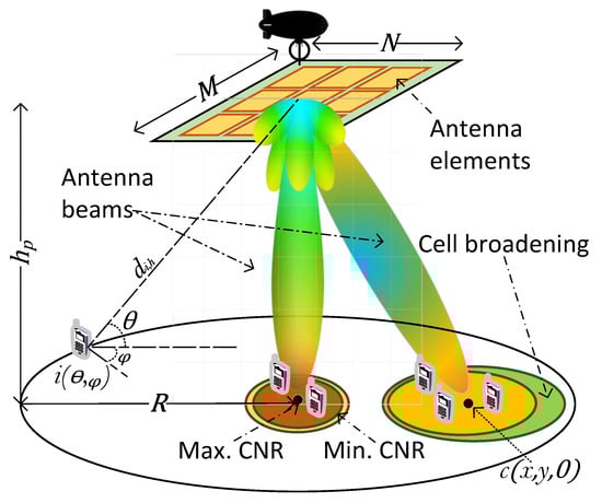
Figure 1.
HAP phased array antenna beamforming for cellular coverage.
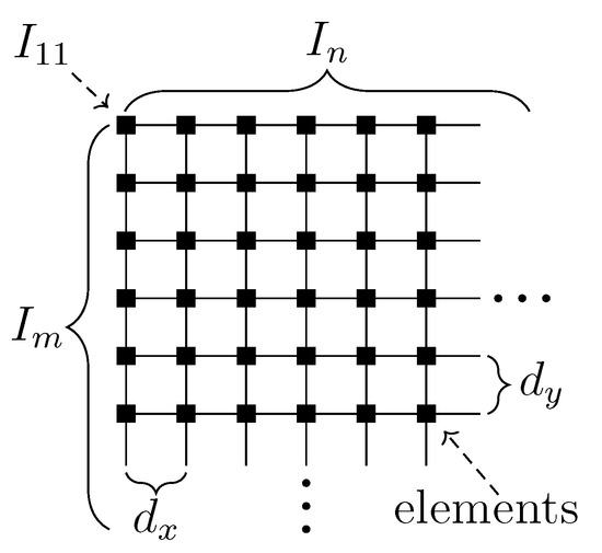
Figure 2.
Antenna element excitation for an antenna array. Elements in rows and columns are referred to as x- and y-axes elements with and distances apart, respectively. There is proportionality between the excitation amplitudes of the elements in both axes. The th element excitation amplitude is expressed as [24].
Coordinates of the multiple beam boresight points on the ground, which are obtained as a set of cell coordinates from the proposed algorithm and then converted into their corresponding elevation and azimuth angles of the HAP from the ground, are supplied to the beamformer implementing (1) to obtain the distribution of HAP antenna transmit gain on the ground. The beams formed are then used to create HAP cells on the ground. In defining a cell in this paper, let be the footprint of the bth beam on the ground, p be any interior point in and be the carrier-to-noise ratio (CNR) at point p, the cell c is a bounded region around the beam boresight with boundary dB. The 9 dB value is a global system for mobile communications (GSM) standard for cell delineation [25], which ensures that every user in a cell can receive signal with good quality. for user i is evaluated as
where is the HAP transmit power, and and are the antenna gain and noise power of the receiver, respectively. The path loss between user i and the HAP h is modelled as free-space path loss with log-normally distributed fading due to shadowing [14], which follows the 3rd generation partnership project (3GPP) non-terrestrial network (NTN) channel model [26] and allows for a realistic large-scale representation of the HAP propagation channel. is expressed as
where is the slant distance between user i and the HAP h in km, f is the carrier frequency in GHz, v is the speed of light in m/s and is a log-normally distributed random variable with zero mean and standard deviation of 4 dB, representing fading due to shadowing [19]. Small-scale fading is not considered in this line-of-sight (LoS) scenario, since the focus is on cellular structure in general and the long-term mutual interference effects of the cells on each other. It is also because the HAP is assumed quasi-stationary and users are fixed; therefore, no small-scale fading is experienced. This is validated by results from a practical HAPS flight test reported in [27].
Cell pointing to achieve good tessellation depends initially on the radius of the SPPC (i.e., the HAP antenna broadside cell), which is defined by the angle subtended by the edge of the SPPC to a plane vertical to the HAP. This depends on the antenna mainlobe beamwidth and the minimum CNR requirement at the edge of the SPPC. Here, is defined such that at all locations within a cell, dB. The HAP antenna array forms multiple beams, which are pointed at a set of coordinates , such that the footprints create a regular tessellated structure of contiguous cells over the entire HAP service area. The cell centre coordinates are supplied by the proposed beam-pointing algorithm discussed in detail in Section 4. The resulting cells in the extended service area are disproportionate in size and shape due to the effect of broadening mainly at low elevation angles.
2.2. User Distribution
Considering a user density of users/km2, a set of users with 2D coordinates are randomly distributed over the HAP service area of A km2. The users in are independently and identically distributed over the space according to a Poisson distributed random variable with mean . The number of users is , where denotes cardinality. This follows a bivariate Poisson point process (PPP) .
User Association
For evaluating the performance of the proposed model, the distributed users are associated to the cells formed using the coordinates obtained from the proposed algorithm. It is important to note that the user distribution does not affect the tessellation performance of the proposed pointing algorithm. The tessellation described in Section 4 is aimed at providing contiguous coverage of cells over the entire service area considering the footprints of the HAP antenna beams. Users are distributed over the service area to assess both the CNR and CINR distribution on the ground resulting from the algorithm’s cell tessellation.
The users associate with cells based on their perceived CNR. User i associates to cell where it achieves the highest CNR, which must be at least equal to a given threshold. If a user’s CNR is less than the threshold in any of the cells, the user is not connected in that cell. Furthermore, if user j is located in a region where two or more cells overlap, it is assigned to the cell that maximises its received power. Invariably, users in an overlap region can detect all the overlapping cells . The set of coordinates of the overlapping cells for all users an overlap region is obtained as follows,
where N is the number of overlapping cells. Then, the set of received powers for user j is defined in (7). User j associates to cell such that realises the maximum in .
2.3. Performance Metrics
In deciding the cell a user should associate with after the formation of cells, and whether service can be provided at a given performance level, the user’s received power, expressed mathematically below, is used. Additionally, other metrics for performance evaluation are presented below.
- CINR : For users already associated to cells, their performance with the proposed algorithm is evaluated using CINR , which expresses the ratio of their carrier power to both interference and noise, which are further described below. For user i, is defined as [14,15]where is the user i’s useful received signal power, is the sum of interference from all interfering beams, and is user i’s thermal noise power, which is a zero mean Gaussian white noise and a function of system temperature and bandwidth (see Section 5 ). is expressed aswhere , is the receive antenna gain given in Section 5, and are as defined in (1) and (5), respectively. For interference, considering full reuse, all non-serving J beams can interfere with user i in the reference beam. The interference on user i in the reference beam from the jth interfering beam iswhere is the jth interfering beam receive power as per (9), and is the leakage antenna gain between the jth interfering beam and user i evaluated using (1)–(3) with and phase shifts based on and denoting the elevation and azimuth angles at the centre of the jth interfering beam [28].
- Throughput : This is evaluated per user in bits/s/Hz using the Truncated Shannon Bound expression as given below [29].where is the implementation loss, dB is the minimum allowed CINR and dB is the CINR resulting in the maximum achievable throughput [15]. is assumed for an acceptable long term evolution (LTE) signal quality [30], while relates to the LTE signal quality mapping with modulation and coding scheme, where maximum capacity is achieved at around 22 dB CINR [31].
- Average Spectral Efficiency : Let the average capacity per user in cell i and the bandwidth allocated to a user in the cell pointed at any given distance be (expression to be derived later) and , respectively. Thus, .
- Average Area Spectral Efficiency : This is the ratio of average spectral efficiency to the area of the cell in bit/s/Hz/km2 for cell i [32,33]. Thus, .
Several notations have been used throughout this paper. Notations part summarises the most prevalent notations used.
3. Capacity and Spectral Efficiency Analysis
In order to objectively assess the limits of extension of the proposed HAP extended coverage, it is important to highlight the theoretical performance bounds of the system. In this section, an expression for the average per-user capacity achievable in cell i pointing at any given distance away from the sub-platform point (SPP) within the HAP service area is derived. Furthermore, an expression for the average ASE in cell i is obtained as a function of . Calculating the average ASE of a cell pointed at a given distance away from the SPP requires the area of the cell, taking the cell geometry and broadening into consideration. In deriving an expression for HAP cell area, it is assumed that the maximum power point is at the centre of the cell. Ideally, this is not exactly the case, especially for cells formed at low elevation angles. The maximum power point, which might not be at the centre of the beam depending on the boresight point distance from SPP, is skewed towards the HAP antenna. This is also exacerbated by the broadening effect. In this paper, we assume that the beam footprint is elliptical in shape to simplify the mathematical analysis. It is important to highlight that this assumption is plausible. Imagine that a beam from the antenna is approximately conical in shape; then, cutting through the cone at an angle using a straight surface gives an elliptical footprint on the ground. The effect of the curvature of the earth is neglected.
For an elliptical cell i pointing at a distance from the SPP, let and represent its semi-major and semi-minor axes, respectively. If is the height of the platform with the other variables retaining their definition from the previous section, the area of cell i is derived as follows. Considering the geometry in Figure 3, and are derived from as given below.
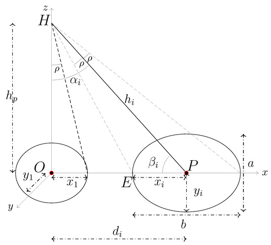
Figure 3.
HAP elliptical cell geometry (semi-major axis).
Using the sum of angles in a triangle rule in , the elevation angle of the HAP from the centre of cell i is,
Hence, using sine rule in , is expressed as follows.
Substituting for in (15),
Using trigonometric identity, (16) can be re-expressed as
Expanding (17),
Therefore, the semi-major axis is expressed as follows.
Furthermore, the semi-minor axis can be derived from Figure 4 redrawn from Figure 3 for convenience.
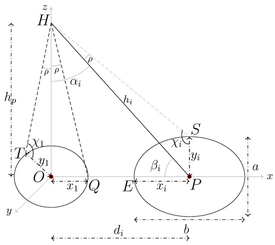
Figure 4.
HAP elliptical cell geometry (semi-minor axis).
Applying the sum of angle in a triangle and sine rules in , yields
and
Thus,
Using (19) and (23), the expression for surface the area of cell i can be obtained. Recall that the area of an ellipse is given as . Thus,
Multiplying (24) by , and using the trigonometric identity , the area of cell i at a given distance from the SPP is derived as
With the expression for the area of a HAP cell i derived, the average capacity per-user and the average ASE in the cell can now be derived. Let be the user-allocated bandwidth. If , , and are the HAP antenna transmit power, transmit antenna gain and receive antenna gain, respectively, is the signal wavelength, is the distance of any arbitrary point from the cell centre at an angle from its x-axis, is the receiver noise density, and is the distance from the boundary to the centre of cell i; is then derived. Considering a uniform distribution of users over cell i, a normalised bandwidth density (in Hz/unit area) detected at position () is expressed as
Hence, the expected capacity density (in bit/s/unit of surface) for a given realisation is defined using the Shannon capacity equation as [34],
where is the CINR at point () in cell i. Considering a user distribution with density in cell i, the average per-user capacity (in bit/s/user) in cell i is expressed as [34]
where denotes the ith cell region. Assuming constant user and bandwidth densities and , respectively, throughout the cell and substituting (27) in (28),
With the assumption of constant user density throughout the cell, the term is eliminated in (29). Thus, the concept of per-user capacity becomes the same as capacity density [34]. Due to the elliptical geometry of the HAP cell, it is more logical to express (29) in polar coordinate form. This involves specifying and in their polar coordinate form. Considering free-space path loss, can be expressed as follows:
Therefore,
where is the slant distance of an arbitrary user in cell i to the HAP. This is based on a single cell scenario, which is noise limited and gives the maximum achievable capacity. needs to be resolved as a function of and , and it is represented in polar coordinates as derived below. This can be achieved by considering the geometry presented in Figure 5.
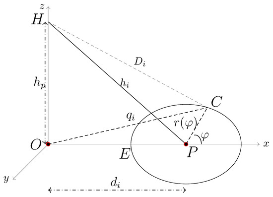
Figure 5.
HAP elliptical cell geometry (polar coordinates).
Imagine that the elliptical cell is flat on the ground and is bounded within a 2D space of radius . The radius varies with respect to the azimuth angle . With origin at the centre of the cell, therefore, is defined as [35]
where e is the cell eccentricity, and are the semi-major and semi-minor axes defined in (19) and (23), respectively. e is expressed as
By applying the cosine rule on in the above figure, can be expressed as a function of . Firstly, the distance of an arbitrary user from the SPP is obtained as follows.
Then, considering and substituting for ,
Unfortunately, there is no closed-form expression for (36). This was the conclusion after trying Chebyshev–Gauss quadrature approximation and using Mathematica, a software tool for mathematical analysis. However, it can be evaluated using numerical methods.
Consequently, the average ASE in cell i is then expressed as
where is the SE. The average ASE highlights the effect of cell broadening on the capacity of a cell, which also skews the maximum power point of a beam away from the centre of the beam, by also considering the cell area. This effect becomes increasingly severe as the HAP service area increases. The degree of service area extension may be based on a given minimum average ASE required, which can be a design parameter. The widely used capacity density metric can be obtained by multiplying the average ASE by bandwidth.
The expressions derived above can be used to model a HAP extended coverage communication system and understand the analytical limit of coverage and capacity extension achievable from a HAP while guaranteeing a minimum QoS. Practically, apart from the shape, size, and capacity of HAP cells, the appropriate placement of the cells plays a key role in minimising interference while enhancing coverage. Section 4 discusses how the disproportionately sized beams due to varied elevation angles can be formed and pointed in practice for better system performance.
4. HAP Beam Pointing for Extended Coverage
This section provides the theoretical framework formulation and detailed discussion of our proposed enhanced and validated algorithm, which is an extension of our conference paper [9]. The algorithm, which aims to exploit the resulting geometry of a HAP beam footprint, gives the total number of cells and a set of their boresight coordinates required to provide extended contiguous coverage and capacity.
4.1. HAP Beam Geometry
The proposed algorithm described in this section considers the geometry of a HAP beam footprint on the ground as shown in Figure 6, which is dependent on the HAP antenna profile and varies in size with the pointing angle. Beams pointing away from the SPP broaden in size due to the limitations of beam forming at lower elevation angles. As discussed in Section 3, we assume that the beam footprint is elliptical in shape. Figure 6 highlights the geometry of the cells with three tessellated cells: one pointed at the SPP and the others at distances away.
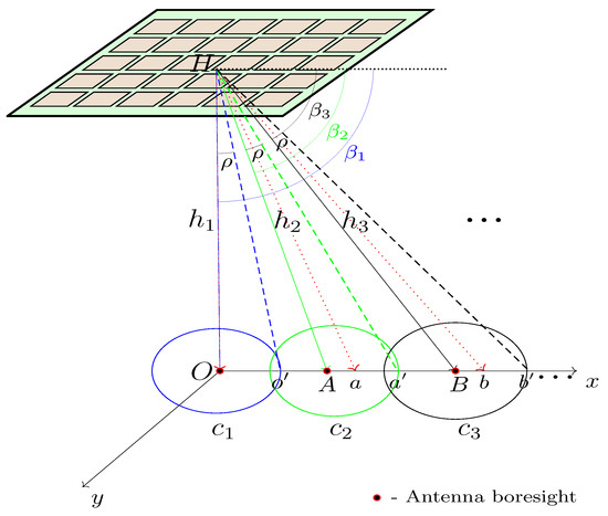
Figure 6.
The HAP cell geometry. Dotted arrow lines show the initial cell boresight when neighbouring cells only touch each other. Solid arrow lines show the new boresight after adjusting the initial pointing angle to add overlap between neighbouring cells. The angle between the solid and dashed lines for each cell highlight the angle between the boresight and cell edge, which is constant.
4.2. Beam-Pointing Algorithm
The proposed algorithm involves five steps, which are described as follows:
- Step 1:
Initially, the boundary of the SPPC is defined by the angle it subtends at the HAP with its centre as highlighted in Figure 6. In addition, the look angle of the cell boresight from the HAP horizontal plane is set to 90. The angle between the cell centre and boundary is assumed to be equal for all cells. Similarly, the initial path distance between the HAP and the SPPC centre is set to . A second cell points along the x-axis of the SPPC by making the angular distance between the centres of and equal to and updated to . A set of the tessellated cell centre coordinates along the x-axis is maintained and updated for each new coordinate. The update of for subsequent cell centres along the x-axis of is carried out using an update function , which is derived as follows.
In order to derive , the geometry shown in Figure 7 is obtained from Figure 6. The solid lines in Figure 7 represent the cell boresight and the dashed lines represent the cell edges. Let be the distances of cell boresights from the SPP along an axis. The distance of cell boresight , i.e., since . Using sine rule on ,
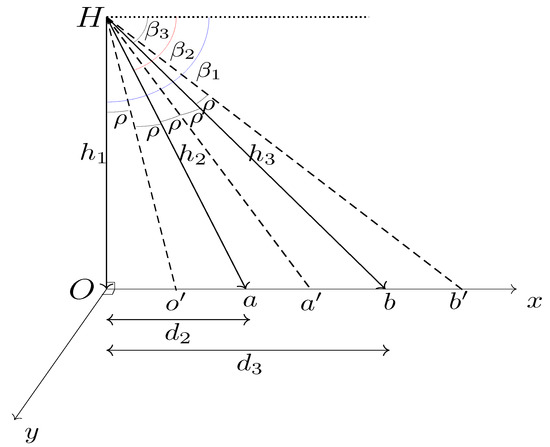
Figure 7.
The HAP cell boresight geometry.
Therefore,
Similarly, the distance of cell boresight . From ,
Thus,
This implies that,
Therefore, a generic equation with a common update function can be obtained from (40) and (43) as
where,
Note that implies that the distance of the SPPC boresight from the SPP is zero and SPPC is the cell at the centre of the HAP service area.
In order to include some level of overlap between and , as depicted in Figure 6, to minimise outage for mobile users moving between cells, the distance between and is reduced by a distance corresponding to an overlap angle , which is a function of the overlap rate and inter-cell distance. The value of between cells and is derived as follows. Consider and in Figure 6 with the geometry partially reproduced in Figure 8.
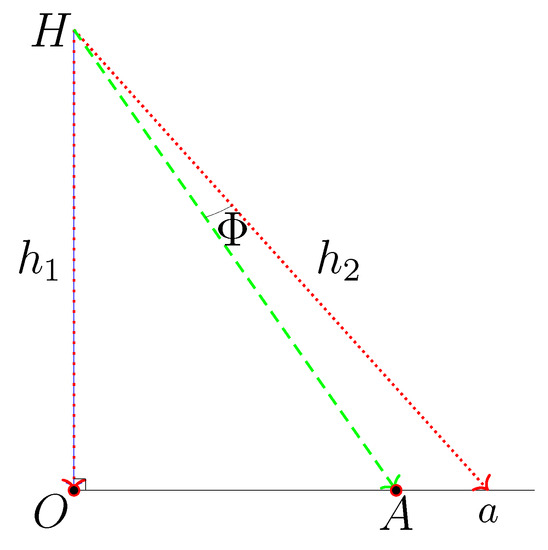
Figure 8.
The HAP cell overlap geometry.
Let be the angle of overlap between neighbouring cells and . Since the coordinate of a is determined based on the size of the SPPC centred at O, can be evaluated while is the platform height. The overlap distance is determined by a given overlap rate and the distance between the neighbouring cell centre boresight from the SPPC boresight. If is the distance of the neighbour to the SPPC and is the distance of the SPPC boresight from the SPP, then
Hence, using the sine rule on and ,
Therefore,
Extending (48) to subsequent cells results in
This process, as described above and depicted in Figure 6, continues for subsequent cells along the x-axis. At the end of this first step, a set of tessellated cell centres is obtained, resulting in the structure shown in Figure 9a. Thus, is defined as follows,
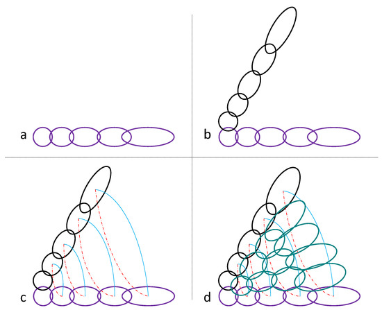
Figure 9.
The cell tessellation processes. (a) The first step with cells pointing at increasing distance on the x-axis. (b) The rotation of the first cells from (a) yielding another set of cells in the second step. (c,d) The third and fourth steps where new cells are deployed between the structure in (b).
- Step 2:
In the second step, all is rotated by 60 as shown in Figure 9b to obtain another set of cell boresight coordinates . The 60 rotation allows for the exploitation of the good tessellation properties of hexagonal geometry. The path vectors between the cells in and their corresponding rotated copies in are obtained using spherical linear interpolation defined by the following expression [36].
where is the angle between corresponding ith cells in and , and are the start and final vectors of the corresponding cells with reference to the SPPC. Meanwhile, represents the path vector between the cells with s determining the steps in the path.
- Steps 3–4:
The solid curve between corresponding cell centre coordinates, as shown in Figure 9c, highlights the paths between the cells and their rotated copies. Ideally, an increasing number of cells will be formed azimuthally on the paths depicted by the solid lines between corresponding cells. These paths are divided into equal path lengths. Here, k indicates the position of the paths, which are shown using the solid lines in Figure 9c, on the cellular arc/path starting from at the SPPC. k new coordinates (equidistant from each other) are introduced starting from arc/path to the last in the structure. However, introducing new cells azimuthally on the solid arcs/paths results in minimal or no overlap between neighbouring cells towards the SPPC. This is due to azimuth antenna pattern (AAP) distortion, which occurs particularly in aerial systems when beams are formed or steered electronically in azimuth using a planar phased array antenna [37,38]. AAP distortion results in steering angle quantisation, grating lobes and main lobe gain reduction [37], which minimises the overlap between neighbouring cells as highlighted earlier. To mitigate against AAP distortion and compensate for the mainlobe gain loss, the new cells are pointed on the mirror images of the paths, which are the dashed convex paths, rather than the original solid concave paths. The mirror image approach, which works by packing the new cells formed azimuthally closer together, is a heuristic and less complex method that ensures proper overlap between neighbouring cells towards the SPPC. The optimality of this heuristic method has not been investigated on this occasion; however, it is shown to enhance the tessellation. A set of the new cell centre coordinates are assigned to to conclude the third and fourth steps with the resulting cellular structure when cells are pointed at these coordinates shown in Figure 9d.
- Step 5:
Finally, in order to achieve full 360 coverage, the union of the set of cell boresight coordinates , and , which yields the tessellation in Figure 9d, is rotated 5 times. The resulting coordinates from the rotation are contained in another set . In Figure 10, a set of the entire cell centre coordinates is therefore obtained as , and the cell footprint is shown. The resulting total number of cells . Note that the proposed algorithm, described in Algorithm 1, is applicable for other antenna beam patterns as long as h, , , and at the SPPC can be defined. The algorithm considers the resulting beam footprints on the ground and not the antenna producing the beams. While the proposed algorithm enables extended HAP coverage, it is important to understand the limits of coverage extension based on the capacity and spectrum performance of the system especially at the edge of coverage. The following section provides a capacity analysis of the extended HAP coverage.
| Algorithm 1: Cell-Pointing Algorithm |
|
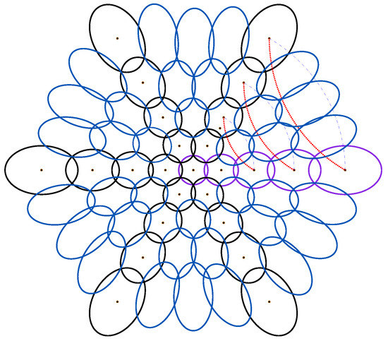
Figure 10.
The full cellular structure for the HAP extended coverage.
Interestingly, Algorithm 1 has much less asymptotic time complexity of in comparison with that of the state-of-the-art in [14], which is , where c, i, and k denote the numbers of cells or K-means centroids declared in [14], users, and K-means iteration respectively.
4.3. Algorithm Validation Using Simulated Annealing
Given the resulting boresight coordinates from Algorithm 1, it is relevant to understand if these locations are near optimum for contiguous and full coverage as part of radio network planning and optimisation. We used SA to validate that the coordinates are near optimum for beam deployment to achieve full coverage.
The implementation of SA for validating Algorithm 1 is similar to the approach proposed in [10]. Firstly, the initial boresight coordinates are set as the resulting coordinates from Algorithm 1. Then, a coordinate is randomly selected and modified as , where and are random scalars drawn from standard normal distribution. Cells are formed using the previous and updated coordinates with users associated to the cells. The sum user CINRs with the previous and updated coordinates are evaluated as and , respectively. If , the coordinate adjustment is accepted; otherwise, it is only accepted with a probability of , where is the temperature of the annealing process. The entire process is repeated with decreased after each run as , where p is the decay factor.
The percentage of coordinates adjusted to improve user CINR compared to the initial coordinates from the proposed beam-pointing algorithm is evaluated for varying T and p and presented in Table 1. Note that only about 5% of the boresight coordinates obtained from the beam-pointing algorithm are adjusted to improve user CINR. This adjustment can be ignored considering the added complexity of running simulated annealing on the overall HAP system with its characteristic energy and weight limitations, and other wider environmental factors that will affect performance, which highlights the practical benefits of the beam-pointing algorithm.

Table 1.
Percentage beam-pointing boresight coordinates modification due to simulated annealing.
5. Performance Evaluation
We set up simulations to evaluate the HAP extended coverage system limits using the derived models and our enhanced beam-pointing algorithm. Simulation parameters are given in Table 2. Using the antenna profile in (1) and 1600 antenna elements [39], it is heuristically determined that the edge-of-cell subtended angle , resulting in an SPPC of approximately 2.5 km diameter. This is used in Algorithm 1 with the resulting cell centre coordinates used as boresights in the antenna system. The CNR and CINR of all users in the service area are evaluated using (4) and (8), respectively. The results are compared with other alternative cell placement schemes.
Table 2.
Details of the simulation parameters.
5.1. Determining Operational Bounds
In order to determine the theoretical bounds of operation of the HAP extended coverage system based on the desired minimum QoS at the edge of coverage, the capacity performance of the derived models in Section 3 is evaluated. The results of the capacity evaluation facilitate the determination of the theoretical bounds of operation of the extended coverage system based on the desired minimum QoS at the coverage edge. To evaluate the average SE of the system, a cell is pointed at increasing distances from the sub-platform point up to the edge of the extended coverage area.
After pointing the cell, the area, average SE, and average ASE are evaluated. The upper and lower limits of the average ASE are obtained. The lower limit is obtained by assuming that all users in the cell have a CNR equal to that of a user at the boundary of the cell (i.e., 9 dB corresponding to the edge-of-cell CNR). This is then used in the Shannon equation (i.e., ) to compute the lower limit average ASE by dividing with the cell area. For the upper limit, it is assumed that all users have a CNR equal to the peak CNR in the CNR distribution, which is the CNR at boresight. This is used in the Shannon equation (i.e., ) to obtain the maximum achievable average SE, which is divided by the cell area to obtain the average ASE. The lower and upper limit average ASE give the bounds of each pointed cell. A different set of average ASE is also obtained by evaluating (36) using numerical integration. The parameters in Table 2 and a 30 dB transmit antenna gain [8] at the boresight are used to simplify the integration and validate the derived expression (36). These average ASE values (i.e., lower limit, upper limit, and integral) are plotted against the distance of the cells from the SPP, as shown in Figure 11. Note that the values represent the best case scenario because they are obtained without considering interference by assuming that the system is only noise limited. In practical systems, the achieved average ASE is expected to be lower when interference is taken into account. The level of interference depends on the number of cells formed and the distance between the cells in addition to the antenna beam profile.
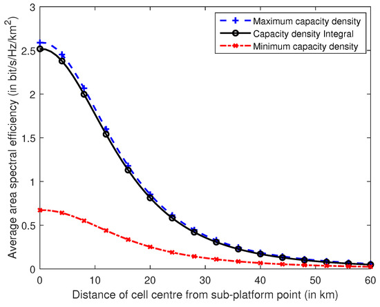
Figure 11.
Average area spectral efficiency against distance of cell centre.
Figure 11 shows the average ASE of cells pointing at increasing distances from the SPP. Notably, the integral average ASE values are close to the maximum because peak transmit gain is used to simplify the (36), as mentioned above. The average ASE reduces with increasing distance from the SPP due to two main factors: increasing path loss and cell area. The number of interfering cells, their proximity to the cell under consideration and the HAP antenna beam profile are some other factors. The average ASE starts tailing-off as the cell centre distance from the SPP approaches 60 km. The value at 60 km is approximately 0.05 bit/s/Hz/km2. If users are allocated a resource block (RB) group each with 750 kHz bandwidth for instance and the area of a cell pointing at the 60 km distance using (25) is evaluated to be approximately 125 km2, the best case achievable capacity of a user in this cell is approximately 4.6 Mbps. Practically, signals at cell edges will be considerably degraded due to ICI. System designers can therefore workout how wide their HAP service area can cover based on the number of cells to be deployed and the required capacity of the edge-of-coverage users. The average ASE values obtained from evaluating (38), as shown in Figure 11, are close to the values obtained when all users in a cell have a signal gain that is equal to the boresight gain. The closeness is expected, as there is a small difference between the boresight gain and the gain at the edge of cell due to small angle subtended () by the cell centre and edge at the HAP.
5.2. Beam-Pointing performance
Having estimated the possible limit of the HAP extended coverage in the previous subsection, we therefore evaluate if it is achievable practically. Heuristically using the antenna profile in (1), it is determined that the edge-of-cell subtended angle , resulting in an SPPC of approximately km diameter. This is used in Algorithm 1 with the resulting cell centre coordinates used as boresights in the antenna module. The CNR and CINR of all users in the service area are evaluated using (4) and (8), respectively. The results are compared with those of regular, equidistant, and equiangular cell placement schemes as well as the state-of-the-art [14].
In the equidistant scheme, cells are pointed such that neighbouring cells are approximately km apart. Figure 12 shows the user CNR contour of the equidistant scheme, with antenna boresights at the centres of the cells. The contour highlights the significant overlap between neighbouring cells resulting from beam broadening. The severe overlap gives rise to high ICI, which worsens at the edges of cells and service area. Therefore, considering beam broadening and overlap is important. Figure 13 shows the user CNR contour with cells pointed such that neighbouring antenna boresights are 7 apart, which is the equiangular scheme. Similarly, this scheme results in severe overlap between cells because it does not explicitly consider beam broadening. The severe overlap and poor CNR, especially towards the edges of cells and coverage area, make these schemes challenging in practical systems due to significant ICI.
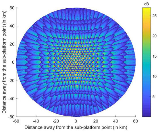
Figure 12.
CNR contour within cells of the equidistant scheme.
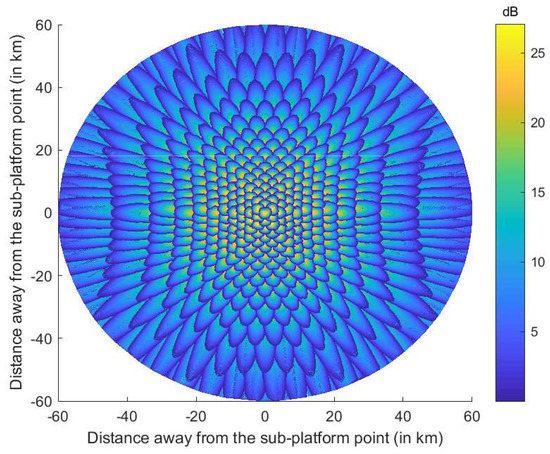
Figure 13.
CNR contour within cells of the equiangular scheme.
Unlike the equidistant and equiangular schemes, Algorithm 1 produces properly structured cells with better overlap control and CNR performance as shown in Figure 14, due to the direct consideration of beam broadening. The algorithm’s CINR performance is also compared with the equidistant and equiangular schemes in addition to schemes proposed in [14]. The empirical CDFs of user CINR distribution obtained with the different cell-pointing schemes are given in Figure 15 and Figure 16. Over 90% of the users using the proposed scheme achieve a CINR greater than 0 dB compared with the the equiangular and equidistant schemes with less than 50% of the users achieving above 0 dB CINR, as shown in Figure 15. The scheme proposed in this section results in a CINR improvement of 7–15 dB. Furthermore, random and regular pointing of cells are presented in [14], as well as the proposed state-of-the-art clustering of users using K-means clustering with cells pointed at the centroid of the clusters. The CDFs of user CINR distributions of these schemes are compared with that of the enhanced and validated scheme proposed. Using the schemes in [14], Figure 16 shows that less than 60% of the users achieve over 0 dB CINR compared with the over 90% obtainable using the proposed scheme with the additional CINR improvement ranging from 5 to 10 dB. Furthermore, Figure 17 highlights the effect of altitude on achievable CINR per user from the proposed scheme. With increasing altitudes, the beam footprint on the ground broadens and CINR per user decreases as more losses occur in the link due to the increasing path distance. Consequently, the spectral efficiency of the system reduces with increasing HAP altitude.
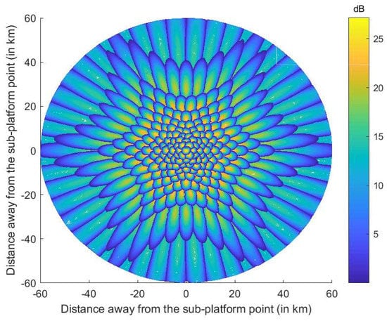
Figure 14.
CNR contour within cells using the proposed scheme.
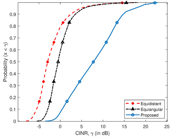
Figure 15.
CINR distribution of the proposed scheme with equidistant and equiangular schemes.
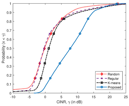
Figure 16.
CINR distribution of the proposed scheme and schemes in [14].
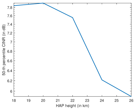
Figure 17.
Platform altitude vs. 50th percentile user CINR.
The effect of overlap ratio on both user allocation probability and 95th percentile user throughput is shown in Figure 18. On the one hand, user allocation probability is evaluated as the ratio of the number of users allocated to a cell to the total number of users. On the other hand, the 95th percentile is obtained by calculating the throughput of all users in the HAP system using (11). The results show that the user allocation probability increases with increasing overlap ratio up to a point beyond which it starts decreasing. This is expected as increasing overlap plugs coverage holes until there are no longer holes within the system coverage. Introducing more overlap at this point starts creating coverage holes, resulting in a decrease in the user allocation probability. Furthermore, the 95th percentile user throughput expectedly decreases with increasing overlap as a result of the increasing ICI, which affects user throughputs. The best value for can be derived as an optimisation problem such that both user allocation probability and user throughput are maximised.
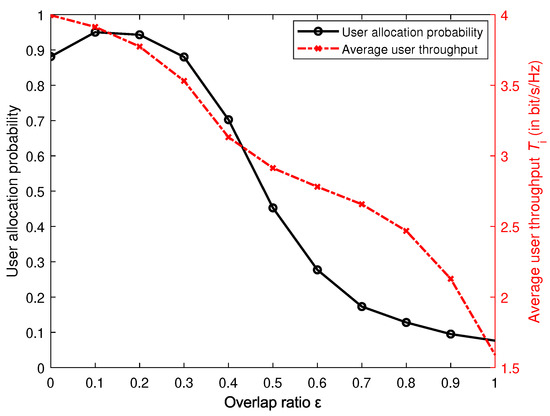
Figure 18.
Overlap ratio vs. user allocation probability and 95th percentile user throughput.
Figure 19 presents the CDFs of the achievable throughput per user for the different cell-pointing schemes, showing the probability that a user achieves a throughput greater than T. It highlights improvements of between 40 and 70% by the proposed scheme compared with the other schemes, with more than 80% of users achieving throughput greater than 1 bit/s/Hz using the proposed scheme compared with about 40% for the state-of-the-art. The improvement is profound because the other algorithms were not developed for extended coverage scenarios; therefore, they do not consider beam broadening, which worsens ICI and results in the poor throughput performance. In Figure 20, the average capacity and CINR per user are shown for the different beam-pointing schemes. Capacity is evaluated using the Shannon equation, as discussed in Section 5.1. Clearly, the figure further highlights the superior performance of the proposed scheme in comparison with the other schemes. The proposed scheme offers an average CINR of over 5 dB and capacity of over 2 bit/s/Hz.
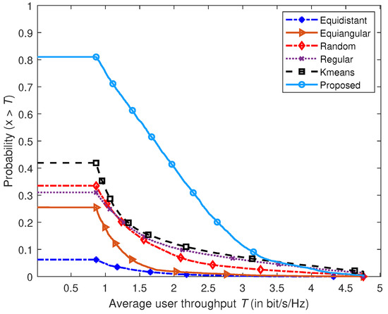
Figure 19.
User throughput distribution of different cell-pointing schemes.
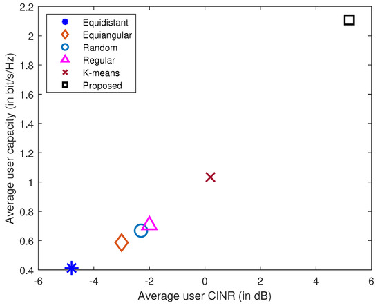
Figure 20.
Average CINR vs. capacity per user of the different schemes.
6. Conclusions
In this work, we estimated the bounds of HAP coverage extension given the operational parameters. Theoretical models for estimating the area and spectral efficiency of an extended HAP coverage area were also derived. By evaluating the average capacity, spectral efficiency, and average area spectral efficiency for cells pointing at increasing distances from the models, we showed that coverage over an extended service area of 60 km radius is achievable. The results show all three variables decrease with increasing sub-platform point distance and that the average area spectral efficiency reduces significantly at extended areas due to the increase in cell size and path loss. Additionally, we enhanced and validated our proposed cell-pointing algorithm to deliver contiguous cellular coverage over an extended service area from a HAP and derived expressions for evaluating the average and area spectral efficiencies for cells pointing at any given location. Simulated annealing verification showed that the algorithm delivered close to optimal cell pointing. The aim was to understand the practicality of an extended HAP coverage. We studied the performance of the algorithm over the estimated 60 km radius service area, using a uniform planar antenna array, which is considerably larger than the area of 30 km radius that much of the HAP-related literature thus far focuses on. It is shown that users in a system using the enhanced and validated scheme achieve CINR values between 5 and 15 dB better than the other schemes with better control of beam overlap. More than of users in our scheme achieve CINR greater than zero as against 45–70% in the compared schemes, which highlights its significant performance improvement.
Author Contributions
Conceptualization, S.C.A., D.G. and P.D.M.; methodology, S.C.A., D.G. and P.D.M.; validation, D.G. and P.D.M.; formal analysis, S.C.A.; investigation, S.C.A.; resources, S.C.A.; data curation, S.C.A.; writing—original draft preparation, S.C.A.; writing—review and editing, D.G. and P.D.M.; visualization, S.C.A.; supervision, D.G. and P.D.M.; project administration, D.G.; funding acquisition, D.G. All authors have read and agreed to the published version of the manuscript.
Funding
This research was carried out by University of York and was partially funded by Orange under research agreement No: H09121.
Acknowledgments
The authors would like to thank Muhammad Danial Zakaria for providing the results of some of the comparative schemes in Section 5.
Conflicts of Interest
The authors declare no conflict of interest.
Abbreviations
The following abbreviations are used in this manuscript:
| AAP | Azimuth Antenna Pattern |
| ASE | Area Spectral Efficiency |
| CNR | Carrier-to-Noise Ratio |
| CINR | Carrier-to-Interference-plus-Noise Ratio |
| HAP | High Altitude Platform |
| ICI | Inter-cell Interference |
| LoS | Line-of-Sight |
| QoS | Quality of Service |
| RB | Resource Block |
| SA | Simulated Annealing |
| SE | Spectral Efficiency |
| SPP | Sub-platform Point |
| SPPC | Sub-platform Point Cell |
Notations
| HAP transmit antenna gain for user i | |
| Receive antenna gain | |
| Path loss between user i and HAP h | |
| Angle subtended at the HAP by a cell centre and edge | |
| Elevation angle of cell i centre to the HAP | |
| Angle of overlap between neighbouring cells | |
| CNR of user i in cell i | |
| CINR of user i in cell i | |
| Average per-user capacity in cell i | |
| Average spectrum efficiency in cell i | |
| Average area spectral efficiency in cell i | |
| Distance of cell i centre from the sub-platform point | |
| Semi-major and semi-minor axes of cell i, respectively | |
| Bandwidth allocated to user i in cell i | |
| Area of cell i | |
| Slant distance of cell i centre from HAP | |
| HAP height | |
| Slant distance of user i in cell i from HAP |
References
- Djuknic, G.M.; Freidenfelds, J.; Okunev, Y. Establishing wireless communications services via High-Altitude Aeronautical Platforms: A concept whose time has come? IEEE Commun. Mag. 1997, 35, 128–135. [Google Scholar] [CrossRef]
- Reynaud, L.; Zaïmi, S.; Gourhant, Y. Competitive assessments for HAP delivery of mobile services in emerging countries. In Proceedings of the 2011 15th International Conference on Intelligence in Next Generation Networks (IEEE ICIN), Berlin, Germany, 4–7 October 2011; pp. 307–312. [Google Scholar]
- Swaminathan, R.; Sharma, S.; Vishwakarma, N.; Madhukumar, A.S. HAPS-Based Relaying for Integrated Space–Air–Ground Networks with Hybrid FSO/RF Communication: A Performance Analysis. IEEE Trans. Aerosp. Electron. Syst. 2021, 57, 1581–1599. [Google Scholar] [CrossRef]
- Arum, S.C.; Grace, D.; Mitchell, P.D. A review of wireless communication using high-altitude platforms for extended coverage and capacity. Comput. Commun. 2020, 157, 232–256. [Google Scholar] [CrossRef]
- Perlman, L.; Wechsler, M. Mobile Coverage and its Impact on Digital Financial Services. SSRN Electron. J. 2019. [Google Scholar] [CrossRef]
- El-Jabu, B.; Steele, R. Cellular communications using aerial platforms. IEEE Trans. Veh. Technol. 2001, 50, 686–700. [Google Scholar] [CrossRef]
- Holis, J.; Grace, D.; Pechac, P. Effect of Antenna Power Roll-Off on the Performance of 3G Cellular Systems from High Altitude Platforms. IEEE Trans. Aerosp. Electron. Syst. 2010, 46, 1468–1477. [Google Scholar] [CrossRef]
- Thornton, J.; Grace, D.; Capstick, M.H.; Tozer, T.C. Optimizing an array of antennas for cellular coverage from a High Altitude Platform. EEE Trans. Wirel. Commun. 2003, 2, 484–492. [Google Scholar] [CrossRef]
- Arum, S.C.; Grace, D.; Mitchell, P.D.; Zakaria, M.D. Beam-Pointing Algorithm for Contiguous High Altitude Platform Cell Formation for Extended Coverage. In Proceedings of the 2019 IEEE 90th Vehicular Technology Conference (VTC2019-Fall), Honolulu, HI, USA, 22–25 September 2019; pp. 1–5. [Google Scholar]
- Yaacoub, E.; Dawy, Z. LTE radio network planning with HetNets: BS placement optimization using simulated annealing. In Proceedings of the MELECON 2014—2014 17th IEEE Mediterranean Electrotechnical Conference, Beirut, Lebanon, 13–16 April 2014; pp. 327–333. [Google Scholar] [CrossRef]
- Thornton, J.; Grace, D.; Spillard, C.; Konefal, T.; Tozer, T.C. Broadband communications from a High-Altitude Platform: The European HeliNet programme. Electron. Commun. Eng. J. 2001, 13, 138–144. [Google Scholar] [CrossRef]
- Dessouky, M.I.; Sharshar, H.A.; Albagory, Y.A. Design of High Altitude Platforms Cellular Communications. Prog. Electromagn. Res. 2007, 67, 251–261. [Google Scholar] [CrossRef]
- Dessouky, M.I.; Sharshar, H.A.; Albagory, Y.A. Geometrical Analysis of High-Altitude Platform’s Cellular Footprint. Prog. Electromagn. Res. 2007, 67, 263–274. [Google Scholar] [CrossRef]
- Zakaria, M.D.; Grace, D.; Mitchell, P.D. Antenna array beamforming strategies for High-Altitude Platform and terrestrial coexistence using K-means clustering. In Proceedings of the 2017 IEEE 13th Malaysia International Conference on Communications (MICC), Johor Bahru, Malaysia, 28–30 November 2017; pp. 259–264. [Google Scholar]
- Zakaria, M.D.; Grace, D.; Mitchell, P.D.; Shami, T.M.; Morozs, N. Exploiting User-Centric Joint Transmission—Coordinated Multipoint with a High Altitude Platform System Architecture. IEEE Access 2019, 7, 38957–38972. [Google Scholar] [CrossRef]
- Hong, T.C.; Ku, B.J.; Park, J.M.; Ahn, D.S.; Jang, Y.S. Capacity of the WCDMA System Using High Altitude Platform Stations. Int. J. Wirel. Inf. Netw. 2006, 13, 5–17. [Google Scholar] [CrossRef]
- Huang, J.J.; Wang, W.T.; Ferng, H.W. Capacity Enhancement for Integrated HAPS-Terrestrial CDMA System. In Proceedings of the 2006 IEEE 63rd Vehicular Technology Conference (IEEE VTC), Melbourne, Australia, 7–10 May 2006; Volume 6, pp. 2597–2601. [Google Scholar]
- Qi, Z.; Jing, X.; You, S. The capacity analysis on a HAPS-CDMA system based on the platform displacement model. In Proceedings of the 2010 2nd IEEE InternationalConference on Network Infrastructure and Digital Content (IEEE IC-NIDC), Beijing, China, 24–26 September 2010; pp. 870–874. [Google Scholar]
- Yang, Z.; Mohammed, A. Deployment and Capacity of Mobile WiMAX from High Altitude Platform. In Proceedings of the 2011 IEEE Vehicular Technology Conference (VTC Fall), San Francisco, CA, USA, 5–8 September 2011; pp. 1–5. [Google Scholar]
- Dong, F.; He, Y.; Nan, H.; Zhang, Z.; Wang, J. System Capacity Analysis on Constellation of Interconnected HAP Networks. In Proceedings of the 2015 IEEE Fifth International Conference on Big Data and Cloud Computing (IEEE CBDCom), Dalian, China, 26–28 August 2015; pp. 154–159. [Google Scholar]
- Ali, A.H. Investigation of indoor Wireless-N radio frequency signal strength. In Proceedings of the 2011 IEEE Symposium on Industrial Electronics and Applications (IEEE ICIEA), Langkawi, Malaysia, 25–28 September 2011; pp. 200–203. [Google Scholar]
- Li, S.; Grace, D.; Liu, Y.; Wei, J.; Ma, D. Overlap Area Assisted Call Admission Control Scheme for Communications System. IEEE Trans. Aerosp. Electron. Syst. 2011, 47, 2911–2920. [Google Scholar] [CrossRef]
- Ganame, H.; Yingzhuang, L.; Ghazzai, H.; Kamissoko, D. 5G Base Station Deployment Perspectives in Millimeter Wave Frequencies Using Meta-Heuristic Algorithms. Electronics 2019, 8, 1318. [Google Scholar] [CrossRef]
- Balanis, C.A. Antenna Theory: Analysis and Design; John Wiley & Sons: New York, NY, USA, 2016. [Google Scholar]
- Oloyede, A.A.; Shamsudeen, A.; Faruk, N.; Olawoyin, L.A.; Popoola, S.I.; Abdulkarim, A. Cost Effective Tri-Band Mobile Phone Jammer for Hospitals Applications. In Proceedings of the IEEE International Rural and Elderly Health Informatics Conference (IREHI 2018), Cotonou, Benin, 3–4 December 2018. [Google Scholar]
- Lin, X.; Rommer, S.; Euler, S.; Yavuz, E.A.; Karlsson, R.S. 5G from Space: An Overview of 3GPP Non-Terrestrial Networks. IEEE Commun. Stand. Mag. 2021, 5, 147–153. [Google Scholar] [CrossRef]
- HAPS Alliance. Bridging the Digital Divide with Aviation in the Stratosphere. 2021. Available online: https://hapsalliance.org/publications/ (accessed on 6 March 2022).
- Kan, X.; Xu, X. Energy- and spectral-efficient power allocation in multi-beam satellites system with co-channel interference. In Proceedings of the 2015 International Conference on Wireless Communications & Signal Processing (WCSP), Nanjing, China, 15–17 October 2015; pp. 1–6. [Google Scholar] [CrossRef]
- Burr, A.; Papadogiannis, A.; Jiang, T. MIMO Truncated Shannon Bound for system level capacity evaluation of wireless networks. In Proceedings of the 2012 IEEE Wireless Communications and Networking Conference Workshops (WCNCW), Paris, France, 1 April 2012; pp. 268–272. [Google Scholar]
- Teltonika. Mobile Signal Strength Recommendations. Available online: https://wiki.teltonika-networks.com/view/Mobile_Signal_Strength_Recommendations (accessed on 31 December 2021).
- Tiong, T. Adaptive Transceivers for Mobile Communications. In Proceedings of the 2014 4th International Conference on Artificial Intelligence with Applications in Engineering and Technology (IEEE ICAIET), Kota Kinabalu, Malaysia, 3–5 December 2014; pp. 275–279. [Google Scholar] [CrossRef]
- Alouini, M.; Goldsmith, A.J. Area spectral efficiency of cellular mobile radio systems. IEEE Trans. Veh. Technol. 1999, 48, 1047–1066. [Google Scholar] [CrossRef]
- Chatzinotas, S.; Imran, M.A.; Tzaras, C. On the Capacity of Variable Density Cellular Systems under Multicell Decoding. IEEE Wirel. Commun. Lett. 2008, 12, 496–498. [Google Scholar] [CrossRef]
- Taranetz, M.; Colom Ikuno, J.; Rupp, M. Capacity density optimization by fractional frequency partitioning. In Proceedings of the 2011 Conference Record of the Forty Fifth Asilomar Conference on Signals, Systems and Computers (ASILOMAR), Pacific Grove, CA, USA, 6–9 November 2011; pp. 1398–1402. [Google Scholar]
- Lawrence, J.D. A Catalog of Special Plane Curves; Courier Corporation: North Chelmsford, MA, USA, 2013. [Google Scholar]
- Barrera, T.; Hast, A.; Bengtsson, E. Incremental Spherical Linear Interpolation. In Proceedings of the Annual SIGRAD Conference Special Theme-Environmental Visualization, Gävle, Sweden, 24–25 November 2004; pp. 7–10. [Google Scholar]
- Xu, W.; Deng, Y.K. Investigation on electronic azimuth beam steering in the spaceborne SAR imaging modes. J. Electromag. Waves Appl. 2011, 25, 2076–2088. [Google Scholar] [CrossRef]
- Zeng, H.C.; Chen, J.; Yang, W.; Zhang, H.J. Impacts of Azimuth Antenna Steering Angle Quantization on TOPS and Sliding Spotlight SAR Image. In Proceedings of the IGARSS 2018—2018 IEEE International Geoscience and Remote Sensing Symposium, Valencia, Spain, 22–27 July 2018; pp. 7813–7816. [Google Scholar] [CrossRef]
- Yang, H.; Yang, F.; Cao, X.; Xu, S.; Gao, J.; Chen, X.; Li, M.; Li, T. A 1600-Element Dual-Frequency Electronically Reconfigurable Reflectarray at X/Ku-Band. IEEE Trans. Antennas Propag. 2017, 65, 3024–3032. [Google Scholar] [CrossRef]
- 3GPP. Evolved Universal Terrestrial Radio Access (E-UTRA); Radio Frequency (RF) System Scenarios. Technical Report 36.942, 3GPP. 2020. Available online: https://www.3gpp.org/ftp/Specs/archive/36_series/36.942/ (accessed on 6 March 2022).


Publisher’s Note: MDPI stays neutral with regard to jurisdictional claims in published maps and institutional affiliations. |
© 2022 by the authors. Licensee MDPI, Basel, Switzerland. This article is an open access article distributed under the terms and conditions of the Creative Commons Attribution (CC BY) license (https://creativecommons.org/licenses/by/4.0/).