Small Defect Detection Based on Local Structure Similarity for Magnetic Tile Surface

Abstract

Surface defect detection is critical in manufacturing magnetic tiles to improve production yield. However, existing detection methods are difficult to use to accurately locate and segment small defects on magnetic tile images, because these defects always occupy extremely low proportions of images, and their visual features are difficult to identify, which means their feature representation for defect detection is quite weak. To address this issue, we propose an effective and feasible detection algorithm for small defects on magnetic tile surfaces. Firstly, based on local structure similarity of magnetic tile surfaces, the image is decomposed into low-rank and sparse matrices for estimating possible defect regions. To accurately locate defect areas while filtering out stains, textures, and noises, the sparse matrix is binarized and used for connected components analysis. Then, pixel values in the defect area are normalized, and the Retinex theory is applied to enhance the contrast between defects and background. Finally, an optimal threshold is determined by an automatic threshold segmentation method to segment the defect areas and edges precisely. Experimental results on a number of magnetic tile samples containing different types of defects demonstrated that the proposed algorithm outperforms the existing methods in terms of all evaluation metrics, showing broad industrial application prospects.

1. Introduction

Developing new energy vehicles is imperative to deal with challenges of the global energy crisis and environmental pollution [1]. The key components of electric vehicles contain batteries, electric motors, and electronic controllers [2], where electric motors serving as the driving device [3] are mainly made of a special material called magnetic tile [4]. The quality of magnetic tile has a significant influence on operation performance, and even a small defect on the surface would pose a potential threat to public safety. However, various defects are easily generated during the production of magnetic tiles. According to the their damage mechanisms, defects can be properly classified into blowhole, cracks, break, fray, etc., of which the first two are the most common and deadliest. Figure 1 shows examples of defects on magnetic tile surfaces.

Small-defect detection on the surface of magnetic tiles has always been an extremely challenging task, with four major barriers: (1) The proportion of a small defect in an image is extremely low, where only limited visual features could be extracted. (2) Low contrast between the defect and the dark magnetic tile surface makes it difficult to accurately identify the location of the defect. (3) The arc-shaped magnetic tile surface after polishing is extremely reflective, resulting in an uneven brightness distribution of the images. (4) Defects are easily buried in stains and fine textures that appear after grinding. Developing small-defect-detection technology suitable for magnetic tile surface images is the key to realizing industrial intelligence, and related research is of great significance to promote the development of new energy vehicles, alleviate the energy crisis, and reduce environmental pollution [5].

Traditional magnetic tile defect detection relying on manual visual inspection has many significant drawbacks such as low efficiency, poor real-time performance, and high cost, which greatly restricts the development of enterprises [7]. In recent years, machine vision has been widely used in industrial fields [8,9,10], and its core functions consist of measurement [11], detection [12,13], recognition [14], classification [15], localization [16,17], segmentation [18,19], and so on. With this trend, a great number of defect detection approaches have been proposed, which can be generally categorized into supervised and unsupervised methods. The former method [20,21] first trains a large amount of data and extracts defect features of images to derive a predictive model, whereas the latter method [22,23] generally uses segmentation [24] or clustering algorithms [25] to divide the image into background and defect regions. These methods perform well on detecting large areas of defects on the surface of magnetic tiles. However, they are always powerless against small defects with only a few pixels. This is because most visual features are difficult to identify/learn from such a tiny size, which means feature representations of small defects are extremely weak.

Small defects on magnetic tiles surfaces are not only common but also fatal. Therefore, an effective solution is urgently needed to detect small defects on the magnetic tile surfaces. To address the above-described challenges, a novel defect detection algorithm is proposed. Firstly, the input magnetic tile image is partitioned based on local structure similarity and then decomposed into sparse and low-rank matrices for estimating possible defect regions. Secondly, the sparse matrix is subjected to a binarization operation and connected domain analysis to further exclude interference from stains and textures, so as to accurately locate the defect areas. Then, the pixel values in the defect area are normalized, and Retinex theory is used to enhance the edge of the region and contrast between the background and the defect. Finally, the automatic threshold segmentation method is used to obtain the optimal threshold to accurately segment the defect area and the edge. The contributions in this article are summarized below:

(1) We develop a novel small-defect detection method based on local structure similarity of magnetic tiles surfaces. Compared with the classical methods used in [26,27,28,29], our method not only identifies small defects that are only a few pixels in size, but also better handles the challenges arising from interference factors of low contrast and uneven pixel intensity distribution.

(2) We evaluate the performance of the proposed method on magnetic tile surface images with crack and blowhole defects. In addition, we compare our method with 11 state-of-the-art methods using 8 performance metrics, including the traditional measures, e.g., accuracy, precision, sensitivity, specificity, MIoU, F-measure (MF) [30], normalized mutual information (NMI), and dice coefficient (DC) [31]. Compared with other leading methods, the proposed algorithm obtained competitive results.

The remainder of our paper is organized as follows. Section 3 gives details of the proposed model. In Section 4, experimental results on a number of magnetic tile samples containing different types of defects are presented. Finally, we conclude the main idea and discuss some future work of our paper.

2. Related Work

Defect detection approaches can be generally categorized into supervised [32,33,34] and unsupervised methods [35,36,37]. The supervised methods train a large amount of data and extracts defect features of images to derive a predictive model, such as deep convolutional networks [20,21]. However, gray or dark magnetic tile surfaces present extremely weak visual information, where small defects, in particular, occupy only a tiny area without obvious visual characteristics, such as blowholes and cracks. Therefore, supervised methods often struggle to extract effective features from defect images, resulting in unsatisfactory defect detection. For example, the mean average precision of the YOLACT depth model proposed by An et al. [38] for crack defect segmentation is only 58.03%. Secondly, detection performance of supervised methods is highly dependent on the scale of data, which has high requirements for computer computing power. It is also difficult to collect a large amount of defect data in the process of industrial production and manufacturing. Finally, supervised methods require data labelling, which consumes man power and material resources.

The unsupervised methods [22,23] generally use segmentation [24] or clustering algorithms [25] to divide the image into background and defect regions. For example, Aiger et al. [39] proposed a phase transformation-based approach to locate defect regions by inverse transformations and adaptive thresholds. Su et al. [40] proposed a feature descriptor to threshold each pixel of the image and further perform similarity analysis and clustering of features of local image blocks to identify defect areas. With the popularity of saliency detection models [41,42], Song et al. [43] combined various constraints such as texture features and edge information to label the obtained salient areas as defects. Although these unsupervised methods achieve great performance on rail defect datasets, they would be ineffective against small-defect detection on magnetic tile surfaces. The main reason is that there are a number of stains and fine texture interferences on magnetic tile surfaces, which are easy to misjudge as defects. Secondly, the brightness distribution of the magnetic tile image is uneven, and the contrast between defect and background is extremely low, making defective areas appear pretty inconspicuous. Some scholars have proposed improving the contrast [44] or eliminating the texture [45] by adopting preprocessing operations before defect detection. For example, Yang et al. [46] combined nonsubsampled shearlet transform and envelope gray level gradient to detect magnetic tile crack defects, but it is quite time-consuming with an average processing time of about 0.5 s per image [6]. Ben et al. [47] proposed an anisotropic diffusion filtering model to eliminate the interference from textures and undesirable artifacts in the normal background area of the magnetic tile image, which has an accuracy of $89\%$ for crack defect detection. Although these methods are able to detect large areas of defects on the surface of magnetic tiles, they are often powerless for small defects lacking obvious visual features.

3. Algorithm Design

We propose an effective approach for small-defect detection on magnetic tile surface. The system framework (Figure 2) includes four procedures:

Step 1: Estimate possible defect areas. The magnetic tile image is partitioned along the vertical direction of texture which exhibits strong similarity, and the input matrix ($I_O$) is reconstructed by the vectorized image block. Based on the sparsity of small defects in the input matrix ($I_O$) and the low rank of the vector composed of image blocks, the input matrix ($I_O$) is decomposed into a sparse matrix ($I_D$) and a low rank matrix ($I_B$), so as to estimate the possible defect regions.

Step 2: Precise locating of defective blocks. By the binarizarion operation and connectivity domain analysis of the sparse matrix, a large amount of interferences, including stains and textures, are further eliminated, so as to accurately locate the defect area.

Step 3: Improve contrast of defective areas. The pixel values in the defect area are normalized, and the Retinex theory is used to enhance the edge of the region and contrast between the background and the defect, which provides a basis for the subsequent accurate determination of pixel attributes.

Step4: Segment defective areas. The optimal segmentation threshold is calculated, and postprocessing operations are performed by connected domain analysis to accurately segment defect areas.

3.1. Estimate Possible Defect Areas

In this section, we chunk the image based on texture features, vectorize the image blocks, then reconstruct a new input matrix, and finally decompose the matrix into low-rank and sparse matrices to estimate possible defect regions. Specifically, the magnetic tile surface image is denoted $I(i,j)$, and its resolution is $M\times N$. Due to the grinding process, magnetic tile surfaces always contain a large number of fine textures. According to the local structural similarity of fine textures, the input image is chunked vertically along the texture, and the resulting image block size is denoted as $dh\times dw$, as shown in Figure 2. The texture of each image block is highly similar, and the image block is further vectorized and used as a column of a new input matrix ($I_O$). Thus, the column vectors would be highly linearly correlated. In addition, the small proportion of small defects on the magnetic tile surface ensures sparsity of the matrix. Based on the above two points, the newly constructed matrix ($I_O$) of the magnetic tile surface image is decomposed into the sum of the low-rank matrix ($I_B$) and the sparse matrix ($I_D$), which is expressed as

$$\begin{array}{c}\hfill I_O=I_B+I_D\end{array}$$

(1)

where the $I_B$ and $I_D$ correspond to the background and defect parts of the magnetic tile surface image, respectively.

Low-rank property of background on magnetic tile surfaces images: To demonstrate that the background of the magnetic tile surface image satisfies the low-rank property, we first select the magnetic tile surface image with uneven brightness distribution and significant interference from stains and textures for the block operation, and then construct the input matrix $I_O$ and calculate its singular value. Figure 3 presents four representative small defects on magnetic tile surface images with the same size of $340\times 240$. The first row is the input image I, and the second row shows the singular value corresponding to the newly constructed matrix $I_O$. Here, we set $dw=240$ and $dh=10$, and then the reconstructed matrix $I_O$ size is $2400\times 34$ with 34 singular values. From the above analysis, it can be seen that as the brightness of the image gradually increases, the first value gradually increases, indicating that the singular value is related to brightness. Although the brightness distribution of all four images is uneven and there issignificant interference from stains and textures, the corresponding singular values all rapidly drop to zero. Therefore, the background of the magnetic tile surface image is low-rank.

Sparseness of small defects on magnetic tile surface images: Assuming that the input image is noise-free, the defect detection task can be transformed into a typical optimization problem of recovering low-rank and sparse components from a data matrix [48]. The process can be formulated as follows:

$$\begin{array}{c}\hfill \begin{array}{cc}\hfill & \hfill \underset{I_D,I_B}{min}rank\left(I_B\right)+\lambda \left|\right|\left(I_D\right){\left|\right|}_0\hfill \\ \hfill & \hfill s.t.I_O=I_B+I_D\hfill \end{array}\end{array}$$

(2)

$$\begin{array}{cc}\hfill & \hfill rank\left(I_B\right)\le r\hfill \end{array}$$

(3)

$$\begin{array}{cc}\hfill & \hfill \left|\right|\left(I_D\right){\left|\right|}_0<k\hfill \end{array}$$

(4)

where $\lambda$ is the weight coefficient ($\lambda >0$), r is a constant, $\left|\right|·{\left|\right|}_0$ represents the $L_0$ norm to count the number of non-zero values, and k is the number of pixels in the defect area. Since the proportion of small-defect region in the image on the surface of the magnetic tile is extremely low, $k\ll M\times N$, the image size is $M\times N$, which means that most elements of the matrix $I_D$ are 0. Therefore, the hypothesis that small defects on the surface of the magnetic tile are sparsity holds.

Decomposition of low-rank and sparse matrices: In order to obtain a convex optimization problem, the $l_0$ norm is relaxed to the $l_1$ norm, and the principal component pursuit method [49] is used to effectively recover $I_B$ and $I_D$, that is,

$$\begin{array}{c}\hfill \begin{array}{cc}\hfill & \hfill \underset{I_D,I_B}{min}\left|\right|\left(I_B\right){\left|\right|}_{*}+\lambda \left|\right|\left(I_D\right){\left|\right|}_1\hfill \\ \hfill & \hfill s.t.I_O=I_B+I_D\hfill \end{array}\end{array}$$

(5)

where $\left|\right|·{\left|\right|}_{*}$ is the nuclear norm of a matrix (i.e., the sum of singular values), and $\left|\right|·{\left|\right|}_1$ is the $L_1$-norm (i.e., the sum of the absolute values of all elements).

In industrial environments, there are often a variety of unknown noises in the magnetic tile surface images, so the noise term is further considered on the basis of the optimization problem Formula (5), and then the stable principal component pursuit method [50] is adopted to solve it, that is,

$$\begin{array}{cc}\hfill & \hfill I_O(i,j)=I_D(i,j)+I_B(i,j))+I_N(i,j))\hfill \end{array}$$

(6)

$$\begin{array}{c}\hfill \begin{array}{cc}\hfill & \hfill \underset{I_D,I_B}{min}\left|\right|\left(I_B\right){\left|\right|}_{*}+\lambda \left|\right|\left(I_D\right){\left|\right|}_1\hfill \\ \hfill & \hfill s.t.\left|\right|I_O-I_B-I_D\left|\right|\le \delta \hfill \end{array}\end{array}$$

(7)

where $\delta >0$, $\left|\right|·{\left|\right|}_F$ is Frobenius norm, that is,

$${\left|\right|X\left|\right|}_F=\sqrt{{\sum }_{ij}{X}_{ij}^2}$$

(8)

To simplify the calculation, the above optimization problem is transformed into the following dual problem [51], that is,

$$\underset{I_D,I_B}{min}\left|\right|\left(I_B\right){\left|\right|}_{*}+\lambda \left|\right|\left(I_D\right){\left|\right|}_1+\frac{1}{2\mu }\left|\right|I_O-I_B-I_D{\left|\right|}_F^2$$

(9)

where $\mu$ is constant and satisfies $\mu >0$. To greatly reduce the amount of computation [52], the appropriate $\mu$ is determined based on the image. Then, the accelerated proximal gradient algorithm [52] and soft threshold operation [53] are used to efficiently solve the duality problem in Equation (9).

The decomposition of the low-rank and sparse matrices in the magnetic tile image has been completed by the above steps, where the sparse matrix contains possible defect regions. In the next section, we will further eliminate interference and precisely locate defective areas.

3.2. Precise Locating of Defective Blocks

Small defects are darker than the background in magnetic tile surface images, which means that they are usually negative in the decomposed sparse matrix. To minimize interference from stains and textures, the defect image is binarized by the following equation:

$$I_D=\left\{\begin{array}{cc}\hfill 1,\hfill & \hfill I_D(x,y)<0\hfill \\ \hfill 0,\hfill & \hfill otherwise\hfill \end{array}\right.$$

(10)

Since the noises of magnetic tile surface images tend to be isolated points, the connected domain pixel value statistical method is further used to quickly remove the noise interference. After locating the defect areas, the remaining area can be directly determined as the background. In the following steps, contrast enhancement and automatic threshold segmentation are only performed on the defect area. If this step is omitted, the subsequent steps require contrast enhancement and defect segmentation of the entire image, in which it is easy to misidentify stains, textures, and black background as defects; it is also time-consuming. Therefore, the operation of defect area positioning in this section not only eliminates the interference such as stains and textures and greatly reduces the time consumption, but also provides a basis for more accurate determination of pixel attributes in the future.

3.3. Improve Contrast of Defective Areas

To improve the contrast between defect area and its surrounding background, pixel values in this area are first normalized, that is,

$$S_k=\sum _{j=0}^k\frac{n_j}{n}k=0,1,2,...,L-1$$

(11)

where $[0,L-1]$ denotes the grayscale range, n is the number of image pixels, and $n_k$ is the number of pixels at the current gray level.

Note that Retinex theory considers not only all possible paths from the random beginning point to the end pixel where the luminance value is calculated, but also tone reproduction and dynamic compression range, which can effectively enhance the local contrast of the image. Based on Equation (11), the multi-scale Retinex theory [54] is used, which can be expressed as follows:

$$R_M=\sum _{m=1}^N{w}_m{R}_{m_i}$$

(12)

where m represents the number of scales. The literature [55] has proved that most images only need 3 scales to achieve great results, that is, $m=3$. $w_m$ is the weight coefficient for each scale. $R_{m_i}$ is defined as follows:

$$R_{m_i}(x,y)=log\left(I_i(x,y)\right)-log(I_i(x,y)•F_m(x,y))$$

(13)

where • represents a convolution operation, $I_i(x,y)$ is the input image for the i-$th$ channel, and $R_i(x,y)$ is the output image after the Retinex algorithm processes the i-$th$ channel. $F_m(x,y)$ is defined as follows:

$$F_m(x,y)=C_m{e}^{-\frac{x^2+y^2}{2{\delta }_m^2}}$$

(14)

where $C_m$ is the normalization constant.

The algorithm proposed in this paper only performs a contrast enhancement operation on the positioned area, which effectively enhances the contrast between the background and the defect area of the image. If contrast enhancement is performed on the whole image, interference information from stains and textures on the magnetic tile surface will be more obvious, which greatly increases the difficulty of defect detection. Therefore, we only perform a contrast enhancement operation on the positioned area, which lays the foundation for the subsequent improvement of defect detection accuracy.

3.4. Segment Defective Areas

After the above steps, the contrast between the defect and background has been enhanced. In this paper, the defect area is further segmented from the localization region. Considering the global information of the locating region, the optimal segmentation threshold $k^{*}$ is calculated, that is [18],

$$k^{*}=arg\underset{1\le k<L}{max}{\sigma }_B^2\left(k\right)$$

(15)

where ${\sigma }_B^2\left(k\right)$ is defined as follows:

$${\sigma }_B^2\left(k\right)=\frac{{[{\mu }_T\omega \left(k\right)-\mu \left(k\right)]}^2}{\omega \left(k\right)[1-\omega (k\left)\right]}$$

(16)

where ${\mu }_T$ is the total average gray of the region, $\omega \left(k\right)$ is the proportion of the top k gray values in the image, and $\omega \left(k\right)$ represents the average gray of the top k gray values.

After obtaining the optimal threshold, the gray value less than the threshold $k^{*}$ is judged as a defect, otherwise as a background, and the expression is as follows:

$$g(x,y)=\left\{\begin{array}{cc}\hfill 1,\hfill & \hfill g(x,y)<k^{*}\hfill \\ \hfill 0,\hfill & \hfill otherwise\hfill \end{array}\right.$$

(17)

Due to the possible interference from factors such as isolated points, the postprocessing operation is carried out by the connection domain analysis to accurately segment the defect area.

3.5. Analysis of Computational Complexity

In this section, the computational complexity of the proposed algorithm is briefly analyzed. As shown in Figure 2, the proposed algorithm is mainly composed of four parts: estimating the possible defect area, accurately locating the defect-containing area, improving the contrast of the positioning area, and segmenting the defect region. In the first step, block first followed by sparse and low-rank matrix decomposition is adopted. The complexity mainly includes singular value decomposition and soft threshold operations, whose values are $O\left(rNM\right)$ and $O\left(NMlog\right(NM\left)\right)$, respectively, where the image size is $M\times N$, and r is the number of singular values. Therefore, the complexity of this step is about $O\left(rLNMlog\right(NM\left)\right)$, where L is the number of iterations. Next, the proposed algorithm locates the area containing defects and then improves the contrast. The complexity lies mainly in the latter step. Assuming that the size of the localized region is $c\times d$, its complexity is $O\left(cdlog\right(cd\left)\right)$. The complexity is $O\left(cd\right)$ in the fourth step. Based on the above analysis, the sum of the complexity of all steps is the overall computational complexity, which is about $O\left(rLNMlog\right(NM)+cdlog(cd)+cd)$ in the proposed algorithm.

4. Experiments

In this section, the commonly used evaluation indicators are introduced to quantitatively evaluate the defect detection effect of the proposed algorithm. We compare them with classical methods to verify the effectiveness and superiority of the proposed algorithm.

4.1. Evaluation Metrics

Commonly used evaluation indicators include accuracy, precision, sensitivity, specificity, MIoU, and F Score (MF), defined as follows:

$$\begin{array}{cc}\hfill & \hfill Accuracy=\frac{TP+TN}{TP+TN+FP+FN}\hfill \end{array}$$

(18)

$$\begin{array}{cc}\hfill & \hfill Precision=\frac{TP}{TP+FP}\hfill \end{array}$$

(19)

$$\begin{array}{cc}\hfill & \hfill Sensitivity=\frac{TP}{TP+FN}\hfill \end{array}$$

(20)

$$\begin{array}{cc}\hfill & \hfill Specificity=\frac{TN}{TN+FP}\hfill \end{array}$$

(21)

$$\begin{array}{cc}\hfill & \hfill MIoU=\frac{TP}{FN+TP+FP}\hfill \end{array}$$

(22)

$$\begin{array}{cc}\hfill & \hfill MF=(1+{\beta }^2)\frac{Pr·Se}{{\beta }^2·Pr+Se}\hfill \end{array}$$

(23)

True positive ($TP$) represents the number of correctly detected defect pixels mapping to the ground truth. True negatives ($TN$) represents the number of correctly detected background pixels mapping to the ground truth. False positive ($FP$) denotes the number of defect pixels that are falsely detected. False negative ($FN$) denotes the number of undetected defect pixels. Sensitivity refers to the probability of defect judgment in the result that is actually a defect. Specificity refers to the probability that the background is correct in the actual background result. MF takes into account both the accuracy and recall of the classification model, which can be regarded as the harmonic average of the model in precision and recall, and ${\beta }^2$ is set to $0.3$ in this paper to pay more attention to precision [30].

In this paper, the model is not only evaluated from the pixel perspective, but also the Normalized Mutual Information $NMI$ is used to quantitatively evaluate the segmentation effect. In addition, the dice coefficient (DC) is an overlap metric that measures the similarity of two sets [31]. Its expression is:

$$DC=\frac{2|A\cap B|}{\left|A\right|+\left|B\right|}$$

(24)

where A and B represent the test image and the ground truth, respectively, both of which are binary images.

4.2. Datasets

In this paper, two publicly available datasets are used in the experiments. The image sizes of different defects in the magnetic tile [6] dataset are different, and the image sizes of the same type of defect are not completely uniform. For this reason, in the experiments in this paper, the defect images of blowhole and crack are cropped to $360\times 260$ and $285\times 125$ pixel sizes, respectively. The average detection time of the proposed algorithm for the two types of defect images is about $0.35$ s and $0.14$ s, respectively. Compared with the average time consumption of $0.5$ s [6] per image by traditional methods, the proposed algorithm has great advantages in calculating time. We also use the AITEX fabric image database https://www.aitex.es/afid/, accessed on 20 December 2022, which contains a number of images with a resolution of $256\times 256$ pixels.

4.3. Performance Comparison with Related Method

In order to verify the effectiveness of the proposed algorithm (denoted as Ours), this paper compares it with the classical methods Ostu [18], OAT [19], EnOstu [26], VE [27], NVE [28], GVE [56], IVE [29], KM [25], MT [21], PHOT [39], SSD [57], GASB [23], and SSA [22]. Ostu [18] and OTA [19] are the methods to automatically obtain image segmentation thresholds, and KM [25] is a clustering algorithm. EnOstu [26] is a fully automated inspection method that not only detects quite small defect areas, but also overcomes the low contrast between defect and defect-free. The VE [27] method has a wide range of applications, from no defects to small or large defects. NVE [28] has accurate segmentation results in defect detection, such as a small-defect image, a number image, and a part image. GVE [56] solves the problem of obtaining the optimal segmentation threshold in unimodal or near-unimodal images by introducing a Gaussian-weighted scheme. IVE [29] effectively solves the problem of defect detection with uneven illumination, complex image texture, and relatively small defect area. MT [21] is a deep fusion model with high accuracy by combining the features of two deep neural networks, i.e., the SqueezeNet and MobileNetV2, giving significant results for multiple rail surface defects under low contrast. PHOT [39] can be applied to defect detection scenarios that contain various types of textures. SSD [57] has the ability to detect various types of defects in smooth backgrounds. GASB [23] is a reconstruction-based method capable of dealing with an isotropic segmentation problem. SSA [22] is an unsupervised autoencoder-based defect segmentation method.

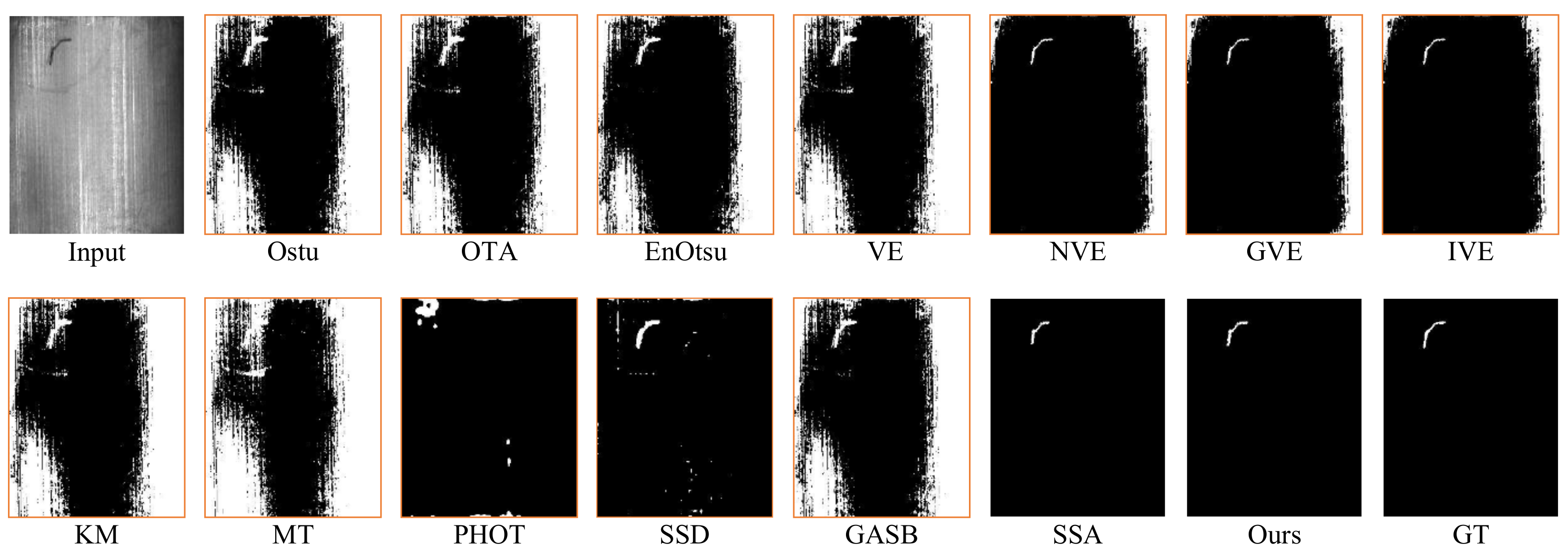
4.3.1. Crack Defect Detect

In this paper, the proposed algorithm is evaluated on the magnetic tile dataset [6] and compared with 13 recently proposed algorithms. The visual comparisons are shown in Figure 4 and Figure 5. Figure 6 shows some quantitative comparison.

We can observe from Figure 4 that Ostu [18], OAT [19], EnOstu [26], VE [27], KM [25], MT [21], PHOT [39], and GASB [23] fail to locate the defect. NVE [28], GVE [56], IVE [29] SSD [57], and SSA [22] are capable of identifying the defect location, but at the same time, some backgrounds are misjudged as defects. Our method is able to effectively separate the defect from the background. To further evaluate the performances of these methods, we conduct experiments on five randomly selected crack defect images, as shown in Figure 5. In this experiment, the results of the Ostu [18], OAT [19], EnOstu [26], VE [27], KM [25], MT [21], PHOT [39], and GASB [23] methods are not present because they are incapable of detecting defects, and their results contain many false positives.

It can be seen that SSD misidentifies part of the background as a defect, and NVE [28], GVE [56], IVE [29], SSA [22] and the proposed method (ours) are suitable for the detection of crack defects by the comparison of the above experiments. Figure 6 shows some quantitative comparisons of the five methods (NVE [28], GVE [56], IVE [29], SSA [22], and our method). As shown in Figure 6a,c,e–h, accuracy, sensitivity, MF, MIoU, DC, and NMI are clearly higher than those of the baseline methods. Specificity represents the probability of detected background pixels, and sensitivity denotes the probability of detected defect pixels. However, it should be noted that recall is more indispensable than precision in surface defect detection, in that a missed defect constitutes a greater hazard than an error-checked noise. The performance comparison demonstrates that the proposed method performs better than all the competitors in detecting the images with crack defects.

4.3.2. Blowhole Defect Detection

The proposed algorithm is evaluated on the small surface defect detection dataset with a blowhole defect and compared with 13 recently proposed algorithms. The visual comparisons are shown in Figure 7 and Figure 8.

Table 1. Results on magnetic tile images in terms of $Ac$(%), $Pr$(%), $Sp$(%), $Se$(%), $MF$, $MIoU$, $Dic$, and $NMI$.

$\mathit{Methods}$	$\mathit{Ac}$(%)	$\mathit{Pr}$(%)	$\mathit{Se}$(%)	$\mathit{Sp}$(%)	$\mathit{MF}$	$\mathit{MIoU}$	$\mathit{Dic}$	$\mathit{NMI}$
EnOtsu	74.615	9.850	78.799	74.613	0.115	0.087	0.144	0.528
NVE	96.089	7.596	18.663	96.245	0.080	0.052	0.088	0.513
GVE	96.089	7.596	18.663	96.245	0.080	0.052	0.088	0.513
IVE	96.089	7.596	18.663	96.245	0.080	0.052	0.088	0.513
SSA	99.928	95.393	70.728	99.993	0.881	0.683	0.810	0.784
Ours	99.966	91.173	90.303	99.982	0.908	0.827	0.904	0.862

shows some quantitative comparison. The results show that the proposed method, an unsupervised method, ranks first on detection of the small defect of the blowhole dataset across different criteria.

From Figure 7, we can see that EnOstu [26], NVE [28], GVE [56], IVE [29], SSA [22], and our method are able to effectively separate the defect from the background. To further evaluate the performances of these methods, we conducted experiments on five randomly selected blowhole defect images, as shown in Figure 8. In the experiment, as we know, with the smaller and smaller defect area contained in the image, NVE [28], GVE [56], and IVE [29] can detect fewer and fewer defect areas until the defect area is tiny and cannot be identified. EnOstu [26] tends to misjudge darker backgrounds as defects. SSA and our detection result are quite close to ground truth.

To quantitatively evaluate the performances of these methods, we conducted experiments on randomly selected blowhole defect images and calculated the average value of indicators, as shown in Table 1. In the experiment, as we know, accuracy, sensitivity, MF, MIoU, DC, and NMI were clearly higher than the SSA method. The performance comparison demonstrates that the proposed method performs better than all the competitors in detecting the images with blowhole defects.

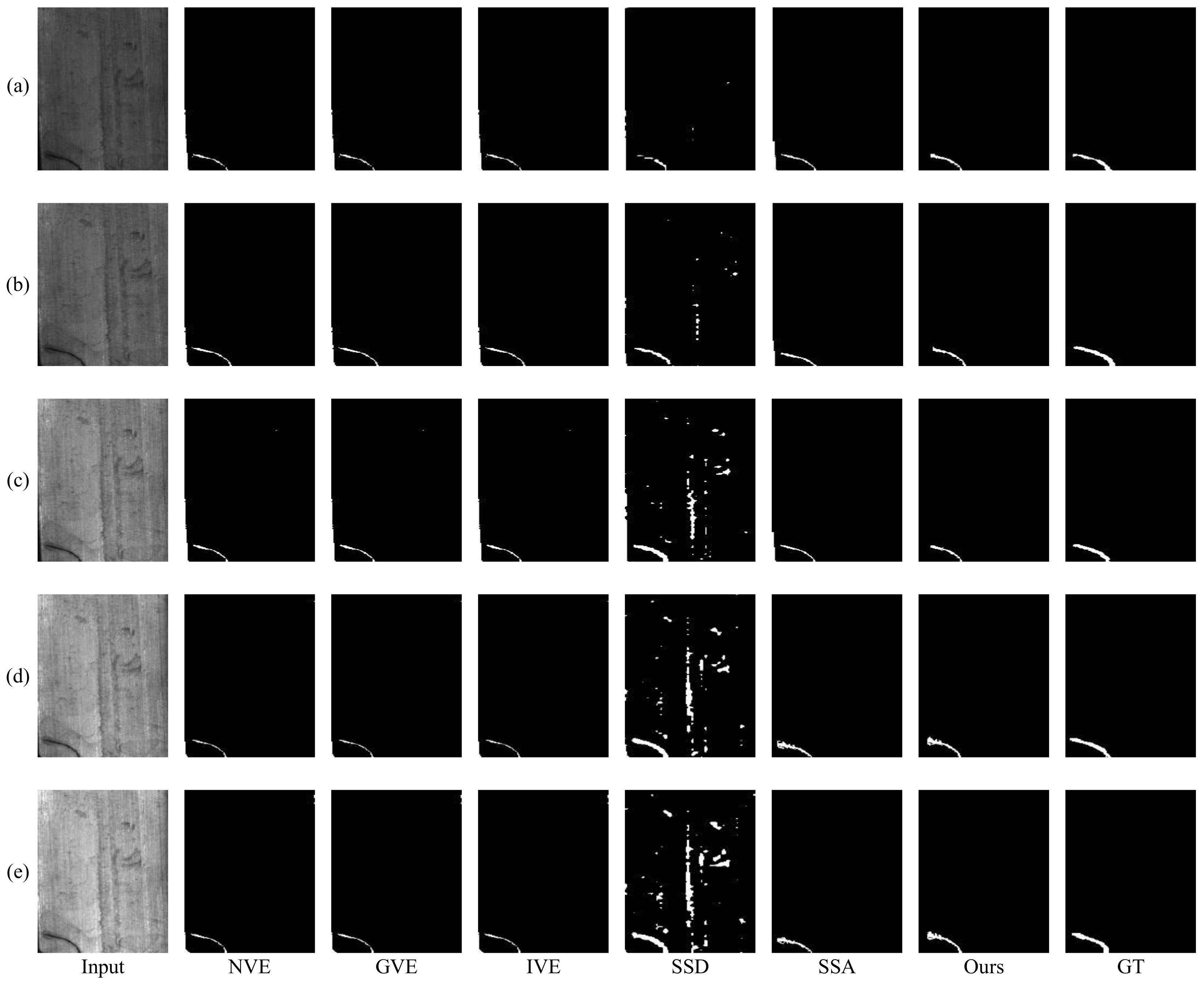
4.3.3. Fabric Defect Detect

We further evaluate the proposed algorithm on the AITEX fabric image database. The visual comparisons are shown in Figure 9, while the quantitative evaluations are present in

Table 2. Results on fabric images in terms of $Ac$(%), $Pr$(%), $Sp$(%), $Se$(%), $MF$, $MIoU$, $Dic$, and $NMI$.

$\mathit{Methods}$	$\mathit{Ac}$(%)	$\mathit{Pr}$(%)	$\mathit{Se}$(%)	$\mathit{Sp}$(%)	$\mathit{MF}$	$\mathit{MIoU}$	$\mathit{Dic}$	$\mathit{NMI}$
Ostu	44.241	0.114	100.000	44.205	0.001	0.001	0.002	0.500
OTA	44.241	0.114	100.000	44.205	0.001	0.001	0.002	0.500
EnOtsu	35.388	0.102	100.000	35.347	0.001	0.001	0.002	0.500
VE	46.073	26.388	91.667	46.032	0.261	0.209	0.258	0.585
NVE	66.664	33.362	35.000	66.670	0.062	0.017	0.032	0.507
GVE	66.664	33.362	35.000	66.670	0.062	0.017	0.032	0.507
IVE	66.664	33.362	35.000	66.670	0.062	0.017	0.032	0.507
kmeans	44.141	0.113	100.000	44.104	0.001	0.001	0.002	0.500
MT	50.447	0.130	99.415	50.415	0.002	0.001	0.003	0.500
PHOT	99.231	0.612	26.667	99.288	0.008	0.006	0.012	0.502
SSD	99.336	39.233	50.117	99.373	0.367	0.248	0.360	0.592
GASB	45.611	0.117	100.000	45.575	0.002	0.001	0.002	0.500
SSA	99.911	45.788	76.111	99.932	0.453	0.326	0.487	0.628
Ours	99.946	63.156	64.865	99.974	0.597	0.419	0.583	0.661

. As can be seen, the Ostu [18], OAT [19], EnOstu [26], VE [27], NVE [28], GVE [56], IVE [29], KM [25], MT [21], PHOT [39], and GASB [23] are all unable to accurately identify the small defect against a fabric surface. Although the SSD [57] and SSA [22] can locate the defect, some backgrounds are misjudged as defects. In contrast, our method is able to effectively separate the defect from the background. In Table 2, we can find that the proposed method significantly outperforms other competing methods by a large margin in terms of all evaluation metrics.

4.3.4. Effects of the Patch Size

In this section, we analyze the influence of the patch size on detection performance of the proposed method. We select 120 images containing defects from 156 defect images which meet the requirements of the area. According to the areas of defects, we divide all targets into six groups where the details of defects are listed in

Table 3. The details of defects in magnetic tile images. The area of a defect is the number of its pixels.

	$\mathit{Group}1$	$\mathit{Group}2$	$\mathit{Group}3$	$\mathit{Group}4$	$\mathit{Group}5$	$\mathit{Group}6$	$\mathbf{The}\mathbf{Whole}$
area	21~40	51~80	81~110	111~140	141~180	181~223	21~223
$\overline{area}$	33	70	102	129	160	206.8	98.6
$\overline{size}$	5.7 × 5.7	8.4 × 8.4	10.1 × 10.1	11.4 × 11.4	12.7 × 12.7	14.4 × 14.4	9.9 × 9.9

. As shown, the defect areas range from 21 (about $4.5\times 4.5$) to 223 pixels (about $15\times 15$). The average area of all 120 defects is $98.6$ pixels, and their average size is $9.9\times 9.9$. The width of the patch is equal to the image width to ensure strong similarity of the partitioned patches along the vertical direction of texture, as can be seen in Figure 2. For quantitative analysis, we fix the width of the patch $dw$ as image width, i.e., $dw=N$, and then change the height of the patch $dh$ as 4, 6, 8, 10, 12, and 14, respectively. The detection accuracy of the proposed method with respect to different patch height is shown in

Table 4. The detection performance of the proposed method (WMD) with respect to different height.

	$\mathit{Group}1$	$\mathit{Group}2$	$\mathit{Group}3$	$\mathit{Group}4$	$\mathit{Group}5$	$\mathit{Group}6$	$\mathbf{The}\mathbf{Whole}$
height $=4$	99.992	99.992	99.990	99.978	99.965	99.932	99.974
height $=6$	99.992	99.992	99.990	99.978	99.964	99.932	99.975
height $=8$	99.992	99.992	99.990	99.978	99.967	99.940	99.977
height $=10$	99.992	99.992	99.990	99.973	99.962	99.927	99.973
height $=12$	99.992	99.961	99.968	99.973	99.964	99.932	99.869
height $=14$	99.983	99.952	99.937	99.973	99.960	99.928	99.861

. As can be seen, the performance of narrow patch is better than that of the broad one when the defects are smaller than $11.4\times 11.4$, i.e., Group 1–Group 4. With the increase of the patch height or defect size, the sparsity and low rank of the patches is difficult to be guaranteed, which leads to the decrease in the detection accuracy. In addition, the proposed achieves the highest accuracy for all the six groups when the patch height is equal to 8. Therefore, we set $dh$ as 8 in the experiments.

5. Conclusions

In this article, we described a model for detecting small defects on magnetic tile surfaces, which is a critical task in the automotive industry. Small blowhole or crack defects occur in the production process, which could lead to potential risks and threaten life. The proposed approach can assist the automotive industry to improve production performance and reduce operation costs by identifying defective magnetic tiles. It mainly consists of four parts: estimating the possible defect area, locating the defect-containing area accurately, improving the contrast of the locating area, and segmenting the defect areas. We showed that our process of locating and then improving contrast and separating defective areas from the background can effectively reduce stains and textures interference, thereby improving recognition rates and reducing time consumption. Experiments on a public dataset showed that our model achieves encouraging performance compared to the state-of-the-art methods. In the future, we will further optimize the model and improve the generalization performance of the algorithm.

References

1. Li, Z.; Khajepour, A.; Song, J. A comprehensive review of the key technologies for pure electric vehicles. Energy 2019, 182, 824–839. [Google Scholar] [CrossRef]
2. Salkuti, S.R. Energy storage and electric vehicles: Technology, operation, challenges, and cost-benefit analysis. Int. J. Adv. Comput. Sci. Appl. 2021, 12, 40–45. [Google Scholar] [CrossRef]
3. Zarma, T.A.; Galadima, A.A.; Aminu, M.A. Review of motors for electrical vehicles. J. Sci. Res. Rep. 2019, 24, 1–6. [Google Scholar] [CrossRef]
4. Cao, X.; Chen, B.; He, W. Unsupervised Defect Segmentation of Magnetic Tile Based on Attention Enhanced Flexible U-Net. IEEE Trans. Instrum. Meas. 2022, 71, 1–10. [Google Scholar] [CrossRef]
5. Xie, L.; Xiang, X.; Xu, H.; Wang, L.; Lin, L.; Yin, G. FFCNN: A deep neural network for surface defect detection of magnetic tile. IEEE Trans. Ind. Electron. 2020, 68, 3506–3516. [Google Scholar] [CrossRef]
6. Huang, Y.; Qiu, C.; Yuan, K. Surface defect saliency of magnetic tile. Vis. Comput. 2020, 36, 85–96. [Google Scholar] [CrossRef]
7. Zhu, Z.; Zhu, P.; Zeng, J.; Qian, X. A Surface Fatal Defect Detection Method for Magnetic Tiles based on Semantic Segmentation and Object Detection: IEEE ITAIC(ISSN:2693-2865). In Proceedings of the 2022 IEEE 10th Joint International Information Technology and Artificial Intelligence Conference (ITAIC), Chongqing, China, 17–19 June 2022; Volume 10, pp. 2580–2586. [Google Scholar] [CrossRef]
8. Adibhatla, V.A.; Huang, Y.C.; Chang, M.C.; Kuo, H.C.; Utekar, A.; Chih, H.C.; Abbod, M.F.; Shieh, J.S. Unsupervised Anomaly Detection in Printed Circuit Boards through Student–Teacher Feature Pyramid Matching. Electronics 2021, 10, 3177. [Google Scholar] [CrossRef]
9. Yang, C.; Luo, J.; Liu, C.; Li, M.; Dai, S.L. Haptics Electromyography Perception and Learning Enhanced Intelligence for Teleoperated Robot. IEEE Trans. Autom. Sci. Eng. 2019, 16, 1512–1521. [Google Scholar] [CrossRef] [Green Version]
10. Ying, H.; Chen, Y. A Neural Network Approach to Subjective Human Face Perception Classification based on Social Characteristics. In Proceedings of the 2021 IEEE 10th Data Driven Control and Learning Systems Conference (DDCLS), Suzhou, China, 14–16 May 2021; pp. 457–462. [Google Scholar] [CrossRef]
11. Zhong, Z.; Ma, Z. A novel defect detection algorithm for flexible integrated circuit package substrates. IEEE Trans. Ind. Electron. 2022, 69, 2117–2126. [Google Scholar] [CrossRef]
12. Wang, H.; Peng, J.; Yue, S. A directionally selective small target motion detecting visual neural network in cluttered backgrounds. IEEE Trans. Cybern. 2018, 50, 1541–1555. [Google Scholar] [CrossRef]
13. Wang, H.; Peng, J.; Zheng, X.; Yue, S. A robust visual system for small target motion detection against cluttered moving backgrounds. IEEE Trans. Neural Netw. Learn. Syst. 2019, 31, 839–853. [Google Scholar] [CrossRef] [PubMed] [Green Version]
14. Alzahrani, A.I.; Ayadi, M.; Asiri, M.M.; Al-Rasheed, A.; Ksibi, A. Detecting the Presence of Malware and Identifying the Type of Cyber Attack Using Deep Learning and VGG-16 Techniques. Electronics 2022, 11, 3665. [Google Scholar] [CrossRef]
15. Li, L.; Xie, N.; Yuan, S. A Federated Learning Framework for Breast Cancer Histopathological Image Classification. Electronics 2022, 11, 3767. [Google Scholar] [CrossRef]
16. Song, Z.; Wang, Y.; Fan, J.; Tan, T.; Zhang, Z. Self-Supervised Predictive Learning: A Negative-Free Method for Sound Source Localization in Visual Scenes. In Proceedings of the IEEE/CVF Conference on Computer Vision and Pattern Recognition, New Orleans, LA, USA, 19–20 June 2022; pp. 3222–3231. [Google Scholar]
17. Feng, G.; Jiang, Z.; Tan, X.; Cheng, F. Hierarchical Clustering-Based Image Retrieval for Indoor Visual Localization. Electronics 2022, 11, 3609. [Google Scholar] [CrossRef]
18. Otsu, N. A threshold selection method from gray-level histograms. IEEE Trans. Syst. Man, Cybern. 1979, 9, 62–66. [Google Scholar] [CrossRef] [Green Version]
19. Bradley, D.; Roth, G. Adaptive thresholding using the integral image. J. Graph. Tools 2007, 12, 13–21. [Google Scholar] [CrossRef]
20. Vrochidou, E.; Sidiropoulos, G.K.; Ouzounis, A.G.; Lampoglou, A.; Tsimperidis, I.; Papakostas, G.A.; Sarafis, I.T.; Kalpakis, V.; Stamkos, A. Towards Robotic Marble Resin Application: Crack Detection on Marble Using Deep Learning. Electronics 2022, 11, 3289. [Google Scholar] [CrossRef]
21. Aydin, I.; Akin, E.; Karakose, M. Defect classification based on deep features for railway tracks in sustainable transportation. Appl. Soft Comput. 2021, 111, 107706. [Google Scholar] [CrossRef]
22. Bergmann, P.; Löwe, S.; Fauser, M.; Sattlegger, D.; Steger, C. Improving Unsupervised Defect Segmentation by Applying Structural Similarity to Autoencoders. In Proceedings of the VISIGRAPP (5: VISAPP), Prague, Czech Republic, 25–27 February 2019. [Google Scholar]
23. Goldstein, T.; Bresson, X.; Osher, S. Geometric applications of the split Bregman method: Segmentation and surface reconstruction. J. Sci. Comput. 2010, 45, 272–293. [Google Scholar] [CrossRef] [Green Version]
24. Oh, C.; Kim, H.; Cho, H. Rotation Estimation and Segmentation for Patterned Image Vision Inspection. Electronics 2021, 10, 3040. [Google Scholar] [CrossRef]
25. Kanungo, T.; Mount, D.M.; Netanyahu, N.S.; Piatko, C.D.; Silverman, R.; Wu, A.Y. An efficient k-means clustering algorithm: Analysis and implementation. IEEE Trans. Pattern Anal. Mach. Intell. 2002, 24, 881–892. [Google Scholar] [CrossRef]
26. Truong, M.T.N.; Kim, S. Automatic image thresholding using Otsu’s method and entropy weighting scheme for surface defect detection. Soft Comput. 2018, 22, 4197–4203. [Google Scholar] [CrossRef]
27. Ng, H.F. Automatic thresholding for defect detection. Pattern Recognit. Lett. 2006, 27, 1644–1649. [Google Scholar] [CrossRef]
28. Fan, J.L.; Lei, B. A modified valley-emphasis method for automatic thresholding. Pattern Recognit. Lett. 2012, 33, 703–708. [Google Scholar] [CrossRef]
29. Liu, Z.; Wang, J.; Zhao, Q.; Li, C. A fabric defect detection algorithm based on improved valley-emphasis method. Res. J. Appl. Sci. Eng. Technol. 2014, 7, 2427–2431. [Google Scholar] [CrossRef]
30. Achanta, R.; Hemami, S.; Estrada, F.; Susstrunk, S. Frequency-tuned salient region detection. In Proceedings of the 2009 IEEE Conference on Computer Vision and Pattern Recognition, Miami, FL, USA, 20–25 June 2009; pp. 1597–1604. [Google Scholar]
31. Dice, L.R. Measures of the amount of ecologic association between species. Ecology 1945, 26, 297–302. [Google Scholar] [CrossRef]
32. Liu, Y.; Xu, J.; Wu, Y. A CISG Method for Internal Defect Detection of Solar Cells in Different Production Processes. IEEE Trans. Ind. Electron. 2022, 69, 8452–8462. [Google Scholar] [CrossRef]
33. Luo, J.; Yang, Z.; Li, S.; Wu, Y. FPCB Surface Defect Detection: A Decoupled Two-Stage Object Detection Framework. IEEE Trans. Instrum. Meas. 2021, 70, 1–11. [Google Scholar] [CrossRef]
34. Dong, H.; Song, K.; He, Y.; Xu, J.; Yan, Y.; Meng, Q. PGA-Net: Pyramid Feature Fusion and Global Context Attention Network for Automated Surface Defect Detection. IEEE Trans. Ind. Inform. 2020, 16, 7448–7458. [Google Scholar] [CrossRef]
35. Liu, W.; Liu, Z.; Wang, H.; Han, Z. An Automated Defect Detection Approach for Catenary Rod-Insulator Textured Surfaces Using Unsupervised Learning. IEEE Trans. Instrum. Meas. 2020, 69, 8411–8423. [Google Scholar] [CrossRef]
36. Mei, S.; Yang, H.; Yin, Z. An Unsupervised-Learning-Based Approach for Automated Defect Inspection on Textured Surfaces. IEEE Trans. Instrum. Meas. 2018, 67, 1266–1277. [Google Scholar] [CrossRef]
37. Niu, M.; Song, K.; Huang, L.; Wang, Q.; Yan, Y.; Meng, Q. Unsupervised Saliency Detection of Rail Surface Defects Using Stereoscopic Images. IEEE Trans. Ind. Inform. 2021, 17, 2271–2281. [Google Scholar] [CrossRef]
38. An, Y.; Lu, Y.; Wu, T. Segmentation Method of Magnetic Tile Surface Defects Based on Deep Learning. Int. J. Comput. Commun. Control 2022, 17, 4502. [Google Scholar] [CrossRef]
39. Aiger, D.; Talbot, H. The phase only transform for unsupervised surface defect detection. In Proceedings of the 2010 IEEE Computer Society Conference on Computer Vision and Pattern Recognition, San Francisco, CA, USA, 13–18 June 2010; pp. 295–302. [Google Scholar]
40. Su, B.; Chen, H.; Zhu, Y.; Liu, W.; Liu, K. Classification of manufacturing defects in multicrystalline solar cells with novel feature descriptor. IEEE Trans. Instrum. Meas. 2019, 68, 4675–4688. [Google Scholar] [CrossRef]
41. Peng, H.; Li, B.; Ling, H.; Hu, W.; Xiong, W.; Maybank, S.J. Salient object detection via structured matrix decomposition. IEEE Trans. Pattern Anal. Mach. Intell. 2016, 39, 818–832. [Google Scholar] [CrossRef] [Green Version]
42. Imamoglu, N.; Lin, W.; Fang, Y. A saliency detection model using low-level features based on wavelet transform. IEEE Trans. Multimed. 2012, 15, 96–105. [Google Scholar] [CrossRef]
43. Song, G.; Song, K.; Yan, Y. Saliency detection for strip steel surface defects using multiple constraints and improved texture features. Opt. Lasers Eng. 2020, 128, 106000. [Google Scholar] [CrossRef]
44. Xie, L.; Lin, L.; Yin, M.; Meng, L.; Yin, G. A novel surface defect inspection algorithm for magnetic tile. Appl. Surf. Sci. 2016, 375, 118–126. [Google Scholar] [CrossRef]
45. Li, X.; Jiang, H.; Yin, G. Detection of surface crack defects on ferrite magnetic tile. Ndt E Int. 2014, 62, 6–13. [Google Scholar] [CrossRef]
46. Yang, C.; Liu, P.; Yin, G.; Wang, L. Crack detection in magnetic tile images using nonsubsampled shearlet transform and envelope gray level gradient. Opt. Laser Technol. 2017, 90, 7–17. [Google Scholar] [CrossRef]
47. Ben Gharsallah, M.; Ben Braiek, E. Defect identification in magnetic tile images using an improved nonlinear diffusion method. Trans. Inst. Meas. Control 2021, 43, 2413–2424. [Google Scholar] [CrossRef]
48. Zhang, H.; Qian, J.; Zhang, B.; Yang, J.; Gong, C.; Wei, Y. Low-Rank Matrix Recovery via Modified Schatten- p Norm Minimization with Convergence Guarantees. IEEE Trans. Image Process. 2020, 29, 3132–3142. [Google Scholar] [CrossRef] [PubMed]
49. Candès, E.J.; Li, X.; Ma, Y.; Wright, J. Robust principal component analysis? J. ACM (JACM) 2011, 58, 1–37. [Google Scholar] [CrossRef]
50. Zhou, Z.; Li, X.; Wright, J.; Candes, E.; Ma, Y. Stable principal component pursuit. In Proceedings of the 2010 IEEE International Symposium on Information Theory, Austin, TX, USA, 13–18 June 2010; pp. 1518–1522. [Google Scholar]
51. Gao, C.; Meng, D.; Yang, Y.; Wang, Y.; Zhou, X.; Hauptmann, A.G. Infrared patch-image model for small target detection in a single image. IEEE Trans. Image Process. 2013, 22, 4996–5009. [Google Scholar] [CrossRef] [PubMed]
52. Lin, Z.; Ganesh, A.; Wright, J.; Wu, L.; Chen, M.; Ma, Y. Fast convex optimization algorithms for exact recovery of a corrupted low-rank matrix. In Coordinated Science Laboratory Report No. UILU-ENG-09-2214, DC-246; Coordinated Science Laboratory, University of Illinois at Urbana-Champaign: Urbana, IL, USA, 2009; Available online: https://core.ac.uk/download/pdf/158319805.pdf (accessed on 10 November 2022).
53. Lin, Z.; Chen, M.; Ma, Y. The augmented lagrange multiplier method for exact recovery of corrupted low-rank matrices. arXiv 2010, arXiv:1009.5055. [Google Scholar]
54. Petro, A.B.; Sbert, C.; Morel, J.M. Multiscale retinex. Image Process. Line 2014, 2014, 71–88. [Google Scholar] [CrossRef]
55. Jobson, D.J.; Rahman, Z.u.; Woodell, G.A. A multiscale retinex for bridging the gap between color images and the human observation of scenes. IEEE Trans. Image Process. 1997, 6, 965–976. [Google Scholar] [CrossRef] [Green Version]
56. Ng, H.F.; Jargalsaikhan, D.; Tsai, H.C.; Lin, C.Y. An improved method for image thresholding based on the valley-emphasis method. In Proceedings of the 2013 Asia-Pacific Signal and Information Processing Association Annual Summit and Conference, Kaohsiung, Taiwan, 29 October–1 November 2013; pp. 1–4. [Google Scholar]
57. Yan, H.; Paynabar, K.; Shi, J. Anomaly detection in images with smooth background via smooth-sparse decomposition. Technometrics 2017, 59, 102–114. [Google Scholar] [CrossRef]
Figure 1. Examples of a magnetic tile surface defect dataset [6]: (a,b) blowhole; (c) crack. The proportion of a small defect is extremely low at the A region, and the brightness distribution of the background is pretty uneven between the B 1 and B 2 regions in (ac); the contrast between the defect and the background is extremely low at the A region in (b); the color of the defect at the A region is extremely similar to the black background at the E region in (a,b); the color of the blowhole defect at the A region and the stains at the C region are highly similar in (a); the crack defect at the A region is similar to the texture structure at the D region in (c).
Electronics 12 00185 g001
Figure 2. Overall flowchart of this paper.
Electronics 12 00185 g002
Figure 3. Low-rank property of (ad) four magnetic tile images. The first row shows four representative examples, while the second is the singular values of the corresponding background patch-images.
Electronics 12 00185 g003
Figure 4. Result of different methods on magnetic tile images with crack defect. Visual comparisons of detection results of the fourteen methods on magnetic tile images with crack defect. NVE, GVE, IVE, SSD, SSA, and the proposed method (ours) are capable of identifying the defect location.
Electronics 12 00185 g004
Figure 5. Visual comparisons of six methods on (ae) five randomly selected crack defect images. NVE, GVE, IVE, SSA, and our method are all close to ground truth.
Electronics 12 00185 g005
Figure 6. Quantitative comparison in terms of (a) accuracy(%), (b) precision(%), (c) sensitivity(%), (d) specificity(%), (e) MF, (f) MIoU, (g) DC, and (h) NMI, where the x axis is Image ID. Our method significantly outperforms these evaluated defect detection algorithms across five randomly selected crack defect images.
Electronics 12 00185 g006
Figure 7. Result of different methods on magnetic tile images with a blowhole defect. Visual comparisons of detection results of the fourteen methods on magnetic tile images witha blowhole defect. EnOstu, NVE, GVE, IVE, SSA, and the proposed method (ours) are capable of identifying the defect location.
Electronics 12 00185 g007
Figure 8. Result of different methods on (ae) five magnetic tile images with a blowhole defect. Visual comparisons of detection results of the six methods on magnetic tile images with a blowhole defect. SSA and the proposed method (ours) are capable of identifying the defect location.
Electronics 12 00185 g008
Figure 9. Visual comparisons of detection results of the fourteen methods on fabric images. SSD, SSA, and the proposed method (ours) are capable of identifying the defect location.
Electronics 12 00185 g009