Abstract
It is difficult for traditional circuit-fault feature-extraction methods to accurately distinguish between nonlinear analog-circuit faults and analog-circuit faults with high fault rates and high diagnostic costs. To solve this problem, this paper proposes a method of mathematical morphology fractal dimension (VMD-MMFD) based on variational mode decomposition for soft-fault feature extraction in analog circuits. First, the signal is decomposed into variational modes to suppress the influence of environmental noise, and multiple high-dimensional eigenmode functions with different center frequencies are obtained. The fractal dimension of the signal feature information component IMF is calculated, and then, KPCA (Kernel Principal Component Analysis) is used to remove the overlapping and redundant parts of the data. The fault set obtained is used as the basis for judging the working state and the fault type of the circuit. The experimental results of the simulation circuits show that this method can be effectively used for circuit-fault diagnosis.
1. Introduction
In daily life and production, circuits can be divided into two types: analog and digital. Although analog circuits generally account for less than 20% of circuit components, 80% of faults are caused by analog circuits [1]. The fault types of analog circuits can be divided into soft faults and hard faults. A hard fault refers to catastrophic faults such as open circuits and short circuits in electronic circuits, which are easy to identify. A soft fault indicates that the value of the components has changed, and the deviation in value exceeds the allowable range [2]. When a soft fault problem occurs, the circuit can still work normally, but if the component is not replaced in time, the soft fault will be upgraded to a hard fault, which will cause significant damage to the entire circuit [3] and even endanger people’s lives and safety.
Many scholars have proposed many feature extraction methods for analog-circuit recognition. Common fault feature extraction methods of analog circuits include principal component analysis [4], factor analysis [5,6], and other linear extraction methods. These methods are relatively effective for linear circuits, but most circuits in daily life have nonlinear features. The above methods cannot reflect the non-stationary characteristics of the signal, resulting in the low separability of the extracted fault features, so there is a large classification error in fault-pattern recognition. Therefore, early soft fault research mainly introduced fuzzy algorithms, wavelet theory, and other means to determine the actual working conditions [7]. Although this algorithm improves the effect of fault diagnosis, some algorithms are seriously affected by the circuit state when analyzing fault characteristics, which makes the performance unstable. In order to solve this problem, in recent years, some scholars have combined mathematical morphology with wavelets and proposed a new nonlinear wavelet morphological wavelet. Reference [8] applied morphological wavelets to detect power disturbance and successfully identified bad conditions in the power transmission process. For example, Zhuang Ning [9] and others combined fractal dimension with EMD (empirical mode decomposition) to extract features of ECG signals to identify different emotional performances. Zheng Zhi [10] and others combined the LMD (local mean decomposition) decomposition method with generalized fractal dimensions to identify gear faults. However, actual measured signals are often accompanied by abnormal events, such as the noise impact and intermittent signals, which lead to modal aliasing and greatly affect the subsequent fault-diagnosis rate. At the same time, a common method to calculate the fractal dimension is the covering method (the box-counting method). This method has inevitable shortcomings. The method itself uses the regular grid division method, so the estimation of the fractal dimension is very unstable in some cases [11].
In view of the above problems, this paper proposes a method to calculate the fractal dimensions (VMD-MMFD-KPCA) of mathematical morphology based on variational mode decomposition (VMD). Using the variational mode decomposition (VMD) of the signal, the interference information in the signal is eliminated to the maximum extent possible to solve the problem of mode aliasing of traditional EMD decomposition. When using morphological fractal dimensions to calculate the dimensions of signals, the instability of traditional box-dimension estimation is avoided, including effectively distinguishing different fault types. On this basis, the KPCA dimension-reduction method is introduced to reduce the dimensions of high-dimensional data calculated by dimensions, eliminate the redundancy and duplication in the sample, and provide a data basis for subsequent fault diagnosis. Compared with traditional fault-diagnosis methods, it shows better performance of feature extraction and diagnosis. Finally, the effectiveness of this method is demonstrated by a simulation circuit.
2. Variational Modal Decomposition
VMD decomposition is a nonrecursive signal-decomposition algorithm. The intrinsic mode function (IMF) in different frequency bands is obtained by adaptively decomposing signals. In the process of solving the mode function, image continuation is used to avoid the endpoint effect in EMD (empirical mode decomposition) and other decomposition methods. VMD’s processing of nonlinear fault signals is helpful for extracting the characteristics of subsequent fault signals. The decomposed IMF has an independent center frequency and sparsity and can effectively avoid mode aliasing when the parameters are appropriate.
(1) In order to obtain a unidirectional spectrum, Hilbert transform is used to analyze and calculate each modal signal, and then the frequency shifting method is used to move the modal spectrum to the baseband:
is the Dirac function; and are the first IMF component and its center frequency decomposed, respectively.
(2) The bandwidth is estimated by the square norm of the gradient, and the constraint expression is:
is the gradient calculation, and * is the convolution calculation symbol.
(3) In order to obtain the optimal solution more efficiently, the constrained problem is transformed into an unconstrained problem by using a Lagrangian operator and penalty factor . The expanded Lagrangian function expression is:
(4) The alternating direction multiplier method is used to iteratively update each modal component and the center frequency, and the saddle point of the unconstrained function is obtained, which is the best solution to the problem. The iterative update expression of , , is as follows:
In Equation (6) is the number of iterations and is the noise tolerance parameter.
(5) Judgment of the iteration termination condition.
where is the judgment accuracy. When > 0, the iteration stops and the cycle ends. The step flow chart is shown in Figure 1:
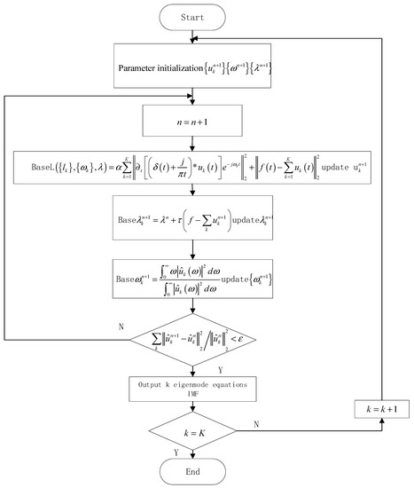
Figure 1.
Variational Modal Decomposition Process.
3. Fractal Dimension Calculation Method Based on Mathematical Morphology
The key to estimating the fractal dimension is to measure the signal at different scales, which can be realized using multi-scale morphology [12]. In the process of gathering and covering the signal, the supremum function, i.e., the structural element g (n), is used for equivalent transformation, and the scale range is analyzed. The algorithm includes two basic operators: expansion and corrosion. For a one-dimensional discrete time signal , the expansion and corrosion results of each scale are, respectively,
where represents corrosion operation; represents expansion operation; represents the structural elements used in the scale ; represents signal; represents a structural element; and is the number of expansion and corrosion. The coverage area of discrete signals at different scales is defined as
When approaches zero, satisfies:
where is the Minkowski–Bouligand dimension of the signal, and c is a constant. The slope of the straight line obtained by a least-square fitting of the above equations and is , which is the final required fractal dimension.
Generally, the unit structure element is chosen to be , because this structure not only ensures that the dimension estimation is not affected by the signal amplitude range but also reduces the computational complexity of the algorithm. In principle, the maximum analysis scale is a positive integer less than ( is the number of discrete signal sampling points). When the data length is relatively large, appropriately reducing can reduce the amount of calculation [13]. In this paper, the length is 256.
4. Kernel Principal Component Analysis
The KPCA method is used to represent the nonlinear relationship between modeling data. It can effectively project linearly indivisible input data into a high-dimensional space that can be linearly separated, and then execute linear in feature space . Assume that the sample set is , where: is the number of samples and is the number of variables. These samples are projected into the feature space through a nonlinear mapping , which can be expressed as:
where is the dimension of the feature space.
The dot product of vector and in feature space H is:
where: k is the kernel function.
The covariance matrix of samples in the high-dimensional feature space H is:
Similar to linear PCA, KPCA in the feature space is equivalent to solving the eigenvalue problem. Let the eigenvector be , the eigenvalue be , and its characteristic equation be:
In Equation (15), each eigenvector in the covariance matrix can be regarded as a linear combination of [14], that is:
where and i are linear correlation coefficients.
Combining Equations (13) and (15), we can obtain
Further simplification results in:
where ; is a kernel matrix, whose eigenvalues are , and the corresponding eigenvectors are . In the feature space , the eigenvector of the covariance matrix in Equation (15) forms a matrix . One principal element (PC) is selected, and we obtain in the principal element space, since the eigenvector should meet the normal constraint in the feature space , that is, . Thus, the eigenvectors of the kernel matrix can be expressed as:
The norm of is taken as the eigenvector, so we have
in feature space H is expressed as
where ;;.
5. Basic Theory of SVM
SVM can provide good generalization performance, and it has been widely used in small-sample classification [15]. As a classical nonlinear problem in the area of fault-location problems, SVM cannot find the classification hyperplane in the original sample space, so it is necessary to introduce a kernel function to map to a linearly separable high-dimensional space. In this paper, a Gaussian kernel function mapping transformation is used, and the expression is as follows:
where, is the square of the distance between and , and r is the super parameter of the kernel function itself:
where is the relaxation variable, is the penalty factor, is the input sample, and is the sample type.
The Lagrangian penalty factor is introduced, and finally the dual type of soft interval Gaussian kernel SVM is obtained as follows:
6. Experiment and Simulation
The method based on VMD-MMFD is used for feature extraction and the fault diagnosis of fault circuits. The specific process is shown in Figure 2.
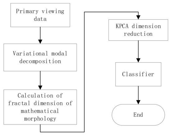
Figure 2.
VMD-MMFD Method Flow Chart.
To verify the effectiveness of this method, simulation experiments and calculations were carried out through the software Multisim, Matlab, and Python. The Sallen–Key band-pass filter circuit was taken as an example to verify the analysis method of soft-fault diagnosis based on variational-mode decomposition and mathematical morphology fractal dimensions. The circuit diagram is shown in Figure 3.
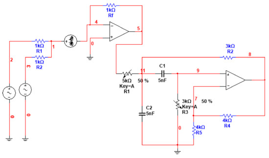
Figure 3.
Sallen−Key band-pass filter circuit.
The excitation signal f = 3sin (30) + 3sin (20) + noise is used as the input source for the fault diagnosis, the tolerance of resistance and capacitance of the circuit is 10%, and the value of components within this range is considered normal. In this experiment, the soft fault state is set when the nominal value fluctuates by 30%. In this experiment, 15-parameter fault combinations are configured. The fault of the amplifier is affected by many factors, so it is not discussed here. The fault mode setting is shown in Table 1, the original signal is shown in Figure 4, the noise signal is shown in Figure 5, and the mixed noise input signal is shown in Figure 6.

Table 1.
Fault Type Description.
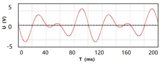
Figure 4.
Original Signal.
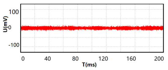
Figure 5.
Noise Signal.
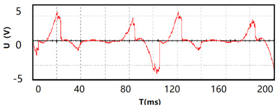
Figure 6.
Input signal of mixed noise.
When VMD is used to decompose signals, the preset scale parameters and the second penalty factor are the main parameters that affect the decomposition accuracy. Therefore, for the VMD decomposition of measured signals, the reasonable selection of its parameters is the difficulty and key of this method. The center frequency of each order of IMF component obtained from the VMD decomposition of the signal is distributed from a low frequency to a high frequency. If the optimal preset scale parameter K is obtained, the center frequency of the last-order IMF component should be the maximum value, and the maximum center frequency value should remain stable. Based on the test and analysis of the VMD decomposition results of a large number of measured signals and reference [16], the second penalty factor is selected in this paper. Take fault type 3 and fault type 5 signals as examples of VMD decomposition, as shown in Figure 7 and Figure 8, the center frequency of the IMF component is obtained by decomposition, as shown in Figure 9 and Figure 10. It can be seen from the figures that when K = 4, the central frequency of the IMF component reaches the maximum and tends to be stable, the frequencies between modes do not overlap, and the impact of noise and mode aliasing is effectively suppressed. With the preset scale parameter K > 4, the center frequencies of IMF 5 and IMF 6 components become unstable and mode aliasing occurs. Therefore, the VMD decomposition of the signal is the best when k = 4.
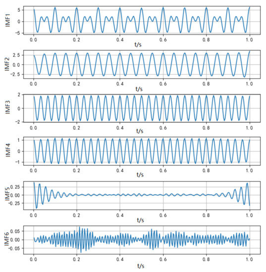
Figure 7.
VMD Decomposition Sequence Diagram of Fault 3 Signal.
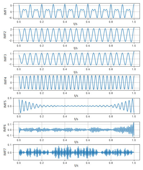
Figure 8.
VMD Decomposition Sequence Diagram of Fault 5 Signal.
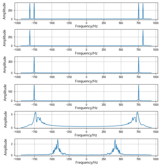
Figure 9.
IMF Component Corresponding Spectrum of Fault 3.
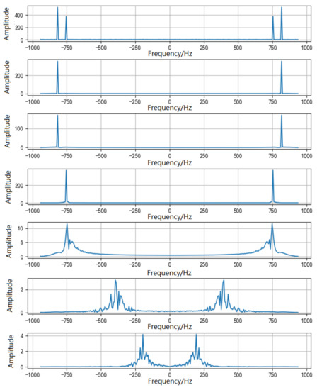
Figure 10.
IMF Component Corresponding Spectrum of Fault 5.
In recent years, in the field of circuit fault diagnosis, the method of combining empirical mode decomposition with box-dimension estimation has been commonly used to extract features [17]. The experiment compares this traditional method with the model of feature extraction based on variational mode decomposition and mathematical morphology. Take four states of types 2–5 as examples, where q is the scale and the value range is [0, 10]. Each state corresponds to 10 fractal dimensions. With the increase in the scale q, fault states are depicted from different dimensions, Dq is the fractal dimension value under different scales q, and the spectrum analysis is carried out.
In Figure 11, the IMF1 component of Fault03 does not overlap with other components, and the IMF1 components of Fault02, Fault04, and Fault05 have aliasing and different degrees of crossing. With the increase in q, the aliasing and crossing become more and more serious, making them difficult to distinguish. In Figure 12, the IMF1 components of Fault02 and Fault04 have serious crossing phenomena, and it is difficult to distinguish the fault types. When the q value is small, the IMF1 of Fault03 and Fault05 have no aliasing phenomena. With the increase in q, the IMF1 of Fault04 has serious cross phenomena with the IMF1 of Fault03 and Fault05. In Figure 13, the IMF1 of Fault04 and Fault05 has seriously crossed, and it is impossible to distinguish the fault type. With the increase in the q value, the IMF1 of Fault03 and Fault04 has also mixed or even crossed phenomena. In Figure 14, when the q value is low, each fault type can be distinguished. With the increase in the q value, the IMF1 of Fault04 and Fault05 has aliasing and crossing phenomena, which affect the discrimination of the fault types. Later, with the increase in the scale of q, the IMF1 of Fault04 and Fault03-IMF1 has a certain degree of aliasing. The characteristic sample set of the IMF1 component dimension of the fault signal is shown in Table 2.

Figure 11.
IMF1-EMD box fractal dimension map.
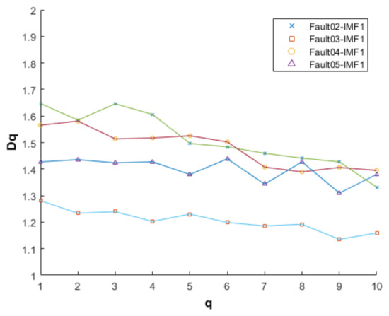
Figure 12.
IMF1-EMD mathematical morphology fractal dimension map.
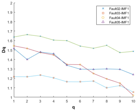
Figure 13.
IMF1-VMD box fractal dimension map.
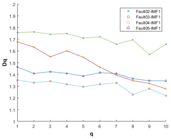
Figure 14.
IMF1-VMD mathematical morphology fractal dimension map.
Table 2.
Characteristic sample of the fault signal analysis dimension.
In Figure 15, the IMF2 of Fault04 and Fault05 has undergone serious aliasing and crossing, and the fault type of the IMF2 of Fault02 and Fault03 can be distinguished, in which aliasing and crossing have occurred. In Figure 16, the IMF2 of Fault02 and Fault03 has been separated, and the fault type is well distinguished, but the IMF2 of Fault04 and Fault05 shows aliasing with the increase in the q value, which is difficult to distinguish. In Fault02 and Fault04 in Figure 17, there is no aliasing, the effect of the fault type discrimination is good, and the IMF2 of Fault02 and Fault04 has serious aliasing and cross phenomena, so it is impossible to distinguish fault types. In Figure 18, when the scale of q is low, the state-differentiation effect of various fault types is good. With the increase in the q value, the IMF2 of Fault02, Fault03, Fault04, and Fault05 shows aliasing and crossing phenomena to different degrees. The characteristic sample set of the IMF2 component dimension of the fault signal is shown in Table 3.
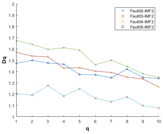
Figure 15.
IMF2-EMD box fractal dimension map.
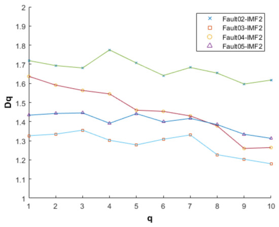
Figure 16.
IMF2-EMD mathematical morphology fractal dimension map.
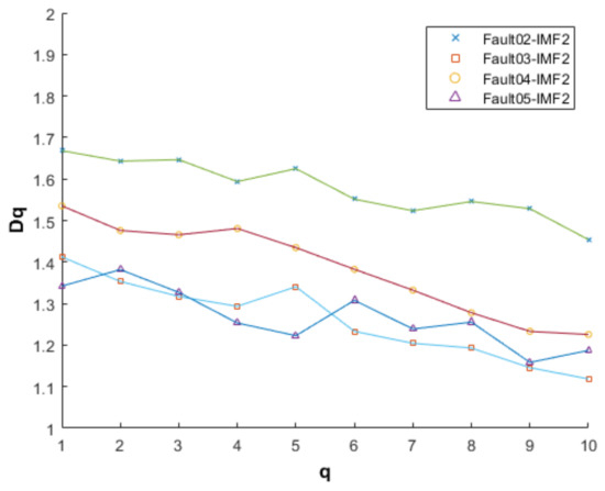
Figure 17.
IMF2-VMD box fractal dimension map.
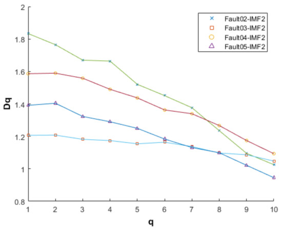
Figure 18.
IMF2-VMD mathematical morphology fractal dimension map.
Table 3.
Characteristic sample of the fault signal analysis dimension.
In Figure 19, with the increase in the number of IMF components, the dimension values of several components of the IMF are no longer stable, because with the increase in the number of modal decomposition components, each component contains less and less original feature information. After the dimension calculation process, the fault types become difficult to distinguish. When the scale of q is small, Fault04 and Fault05 have been aliased and crossed to some extent. With the increase in the scale of the q value, the IMF3 of Fault02, Fault04, and Fault05 has been aliased and crossed to some extent. In Figure 20, the IMF3 aliasing of Fault02, Fault03, Fault04, and Fault05 is obviously crossed, which makes it difficult to distinguish the fault type*. In Figure 21, the IMF3 fault type * of Fault02 is not aliased with other components, and the IMF3 of Fault03, Fault04, and Fault05 is completely aliased, so the fault types cannot be distinguished. In Figure 22, the IMF3 of Fault03 and Fault05 is seriously aliased and crossed, which makes it impossible to classify fault types. The IMF3 of Fault04 and Fault02 is aliased and crossed with the increase in the scale of q, which makes it difficult to classify faults. The sample set of dimension characteristics of the IMF3 components of fault signals is shown in Table 4.
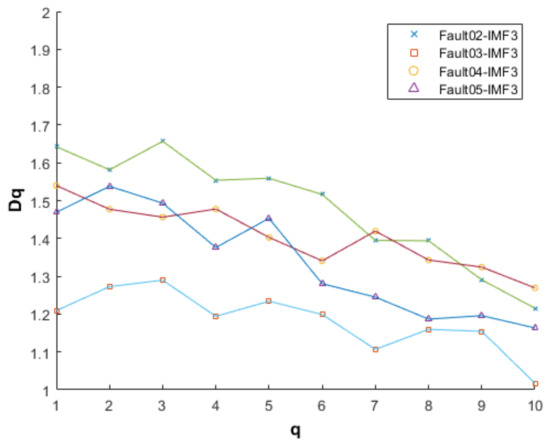
Figure 19.
IMF3-EMD box fractal dimension map.
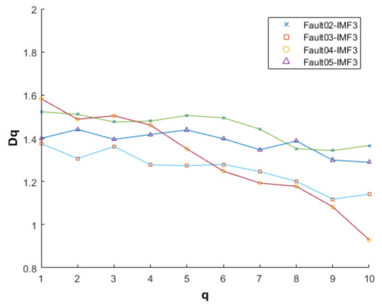
Figure 20.
IMF3-EMD mathematical morphology fractal dimension map.
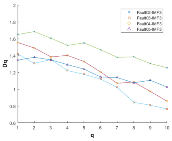
Figure 21.
IMF3-VMD box fractal dimension map.
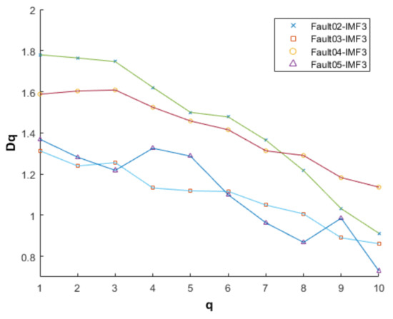
Figure 22.
IMF3-VMD mathematical morphology fractal dimension map.
Table 4.
Characteristic sample of the fault signal analysis dimension.
In Figure 23, with the increase in the number of IMF components, the dimension values of several IMF components fluctuate seriously, and the IMFs of Fault02, Fault03, Fault04, and Fault05 have all experienced serious aliasing and crossing. In Figure 24, the IMF4 in Fault02, Fault04, and Fault05 is aliased, so it is impossible to distinguish the fault type, and with the increase in the q value, the IMF3 in Fault03 is also aliased. In Figure 25, the IMF4 of Fault02, Fault04, and Fault05 shows serious aliasing and cross phenomena and even overlaps with the increase in the scale q, making it difficult to determine the fault type. Only the fault type of the IMF4 of Fault03 can be distinguished. In Figure 26, the IMF dimension maps of the four fault states fluctuate unstably, and the IMF4 of Fault02, Fault03, Fault04, and Fault05 is seriously aliased and crossed, making it impossible to judge the fault type. The characteristic sample set of the IMF4 component dimension of the fault signal is shown in Table 5.
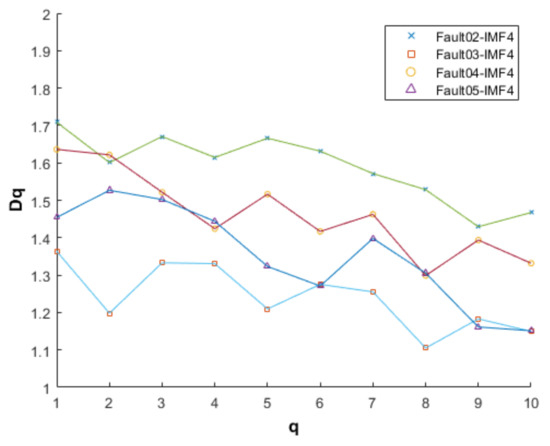
Figure 23.
IMF4-EMD box fractal dimension map.
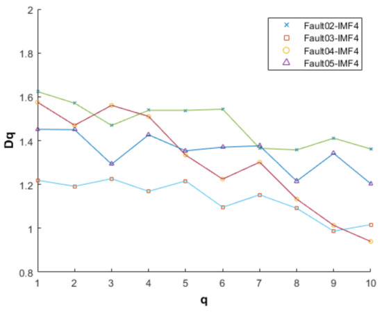
Figure 24.
IMF4-EMD mathematical morphology fractal dimension map.
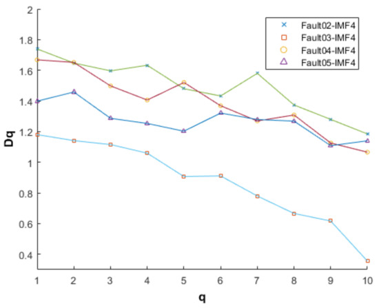
Figure 25.
IMF4-VMD box fractal dimension map.
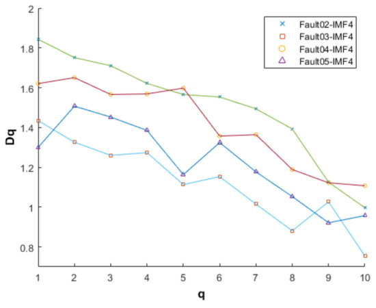
Figure 26.
IMF4-VMD mathematical morphology fractal dimension map.
Table 5.
Characteristic sample of the fault signal analysis dimension.
The feature extraction of different states of signals is carried out through the fractal dimension. Although the number of data samples increases and the fault set becomes larger, the high-dimensional data contain a lot of miscellaneous and repetitive data, which seriously affect the accuracy of fault diagnosis. The feature set needs to be dimensionally reduced. In the literature [18], different kernel functions have different effects on data dimensionality reduction. Generally, the Gaussian radial basis function (Formula (25)) is selected to perform the kernel function PCA on data sets to achieve dimensionality reduction and fault classification in high-dimensional feature space.
The cumulative contribution rate of the principal component calculated by the KPCA algorithm is shown in Table 6. It can be seen from Table 6 that the first three principal components contain almost all the information of the system, so the first three principal components are retained as the eigenvalues of the system; that is, the feature space is reduced from high-dimensional to three-dimensional. KPCA can be used to calculate the principal component contribution rate, effectively eliminating the samples containing too much interference information, which greatly improves the accuracy of subsequent diagnoses.
Table 6.
Cumulative contribution rate.
Therefore, considering the feature extraction method of the VMD-MMFD-KPCA, the results are shown in Figure 27, and various fault types can be distinguished in the following figure.
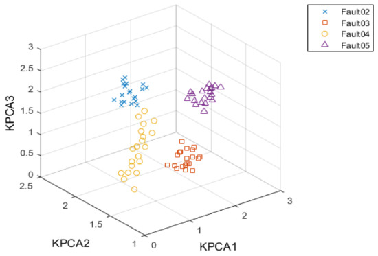
Figure 27.
VMD-MMFD-KPCA feature extraction.
To further verify the effectiveness of the feature-extraction methods explained above, a support vector machine was used to complete fault diagnosis. Among them, the fault datasets that were used were all from the fault settings of various components of the simulation circuit. To achieve better experimental results, more than 50 signal samples were collected for each fault type, and more than 750 signal samples were collected for 15 fault types. Eighty percent of the samples from each fault type were randomly selected as the training sample, and the rest were selected as the test sample. The kernel function was introduced and determined in the previous theory, using Gaussian kernel function. After that, the data needed to be normalized. First, the data need to be filtered and sorted. For obviously abnormal data, we considered using the sample mean to replace it, so as to reduce the extent to which the abnormal sample data interferes with the results. To prevent the individual abnormal sample data volume from influencing the training results, the data were normalized according to Formula (26).
After 100 iterations, diagnosis is carried out in combination with different diagnosis models, as shown in Figure 28.
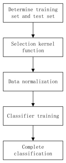
Figure 28.
Flow chart of SVM Classification.
In the literature [19], there is a wavelet neural network (WNN) analog circuit soft fault diagnosis method based on kernel partial least square (KPLS) feature extraction, which uses support vector machine (KPLS-WNN-SVM) for fault classification. In the literature [20], a multifractal extraction method based on empirical mode decomposition is combined with support vector machine (EMD-MFD-SVM). The diagnostic rate of the diagnostic model combined with support vector machine (VMD-MMFD-KPCA-SVM) in this paper is shown in Table 7, which shows that the VMD-MMFD-KPCA-SVM method has the highest diagnostic accuracy.
Table 7.
Fault Diagnosis Rate.
7. Conclusions
This paper proposes a feature-extraction method based on VMD-MMFD-KPCA. Firstly, the fault signal is decomposed by VMD to obtain multiple modal IMF components, which greatly reduces the impact of modal aliasing. The appropriate IMF components were selected, and the fractal dimension of the mathematical morphology was calculated to obtain a large number of high-dimensional feature data sets. The data sets were reduced by KPCA to obtain low-dimensional data, which eliminated a large number of redundant and jumbled information in the high-dimensional data. The experimental results show that the feature-extraction method based on VMD-MMFD-KPCA has a good effect.
Author Contributions
Conceptualization, X.L.; methodology, X.L.; software, S.S.; validation, X.L., K.L., Q.W. and D.S.; writing—original draft preparation, C.Y., Z.L. and J.W.; writing—review and editing, C.Y.; project administration, X.L.; funding acquisition, X.L. All authors have read and agreed to the published version of the manuscript.
Funding
This research was funded by Heilongjiang Provincial Natural Science Foundation of China, grant number YQ2022F014.
Acknowledgments
The authors acknowledge Heilongjiang Provincial Natural Science Foundation of China (grant number YQ2022F014).
Conflicts of Interest
The authors declare no conflict of interest.
References
- Peng, W.; Yang, S. A new diagnosis approach for handling tolerance in analog and mixed-signal circuits by using fuzzy math. IEEE Trans. Circuits Syst. I Regul. Pap. 2005, 52, 2118–2127. [Google Scholar] [CrossRef]
- Zhu, Y.J.; Zhang, W.M.; Zhang, S.T.; Chen, J.J. Judgment and handling of “soft fault” of discrete component circuit. Chin. Sci. Technol. J. Database Eng. Technol. 2016, 9, 00300. [Google Scholar]
- Lu, X.M.; Zhao, H.; Wu, Q. Research on fractal method for soft fault diagnosis of nonlinear analog circuits. Model. Meas. Control. A 2017, 90, 58–73. [Google Scholar] [CrossRef]
- Han, H.T.; Ma, H.G.; Cao, J.F.; Zhang, J.L. Analog circuit fault diagnosis method based on nonlinear spectrum characteristics and kernel principal component analysis. J. Electr. Technol. 2012, 27, 248–2544. [Google Scholar]
- Wang, Y.H.; Lu, J.; Pan, G.Q.; Feng, J.C. Research on Feature Extraction for Diagnostics of Analog Circuit Based on Factor Analysis. Comput. Meas. Control 2014, 11, 25–27. [Google Scholar]
- Xiao, Y.; Feng, L. A novel neural-network approach of analog fault diagnosis based on kernel discriminant analysis and particle swarm optimization. Appl. Soft Comput. 2012, 12, 904–920. [Google Scholar] [CrossRef]
- Guo, Q.; Zhang, W.B.; Su, H.T. Analog circuit fault diagnosis based on WPT and FOAGRNN. Comput. Simul. 2020, 37, 355–359. [Google Scholar]
- Ji, T.Y.; Lu, Z.; Wu, Q.H. Detection of power disturbances using morphological gradient wavelet. Signal Process. 2008, 88, 255–267. [Google Scholar] [CrossRef]
- Zhuang, N.; Zeng, Y.; Tong, L.; Zhang, C.; Zhang, H.; Yan, B. Emotion Recognition from EEG Signals Using Multidimensional Information in EMD Domain. Biomed Res. Int. 2017, 2017, 317–357. [Google Scholar] [CrossRef] [PubMed]
- Zheng, Z.; Jiang, W.L.; Wang, Z.W.; Zhu, Y.; Yang, K. Gear fault diagnosis method based on local mean decomposition and generalized morphological fractal dimensions. Mech. Mach. Theory 2015, 91, 151–167. [Google Scholar] [CrossRef]
- Nayak, S.R.; Mishra, J. Fractal Dimension Based Generalized Box-Counting Technique with Application to Grayscale Images. Fractals 2020, 3, 8. [Google Scholar] [CrossRef]
- Zhang, K.; Cheng, J.S.; Yang, Y. A rolling bearing fault diagnosis method based on local mean decomposition and morphological fractal dimension. J. Vib. Shock. 2013, 32, 90–94. [Google Scholar]
- Wang, F.J.; Duan, S.L.; Yu, H.L.; Li, H.K. Diesel Engine Fault Diagnosis Based on EEMD and Morphological Fractal Dimension. J. Intern. Combust. Engine 2012, 30, 557–562. [Google Scholar]
- Yang, G.; Gu, X. Fault Diagnosis of Complex Chemical Processes Based on Enhanced Naive Bayesian Method. IEEE Trans. Instrum. Meas. 2020, 69, 4649–4658. [Google Scholar] [CrossRef]
- Gashteroodkhani, O.A.; Majidi, M.; Etezadi-Amoli, M.; Nematollahi, A.F.; Vahidi, B. A hybrid SVM-TT transform-based method for fault location in hybrid transmission lines with underground cables. Electr. Power Syst. Res. 2019, 170, 205–214. [Google Scholar] [CrossRef]
- Tang, G.J.; Wang, X.L. Variational modal decomposition method and its application in early fault diagnosis of rolling bearings. J. Vib. Eng. 2016, 29, 11. [Google Scholar]
- Han, D.Y.; Li, G.; Shi, P.M. Research on coupling fault diagnosis method of rotating machinery based on EMD and fractal box dimension. Vib. Shock. 2013, 32, 209–214. [Google Scholar]
- Li, C.Y.; Liu, G.D.; Tan, B. Comparative study of hyperspectral remote sensing data dimensionality reduction based on PCA and KPCA. Geospat. Inf. 2022, 20, 89–93+103. [Google Scholar]
- Cong, W.; Jing, B.; Yu, H.K. WNN soft fault diagnosis of analog circuit based on KPLS feature extraction. J. Cent. South Univ. (Sci. Technol.) 2014, 45, 1841–1846. [Google Scholar]
- Lu, X.M.; Zhao, H.; Wu, Q. Generalized Multi-fractal Method for Soft Fault Feature Extraction of Non-linear Analog Circuits Based on EMD. Rev. De La Fac. De Ing. 2016, 31, 192–203. [Google Scholar]


Disclaimer/Publisher’s Note: The statements, opinions and data contained in all publications are solely those of the individual author(s) and contributor(s) and not of MDPI and/or the editor(s). MDPI and/or the editor(s) disclaim responsibility for any injury to people or property resulting from any ideas, methods, instructions or products referred to in the content. |
© 2022 by the authors. Licensee MDPI, Basel, Switzerland. This article is an open access article distributed under the terms and conditions of the Creative Commons Attribution (CC BY) license (https://creativecommons.org/licenses/by/4.0/).