Tone Mapping Method Based on the Least Squares Method

Abstract

Tone mapping is used to compress the dynamic range of image data without distortion. To compress the dynamic range of HDR images and prevent halo artifacts, a tone mapping method is proposed based on the least squares method. Our method first uses weights for the estimation of the illumination, and the image detail layer is obtained by the Retinex model. Then, a global tone mapping function with the parameter is used to compress the dynamic range, and the parameter is obtained by fitting the function to the histogram equalization. Finally, the detail layer and the illumination layer are fused to obtain the LDR image. The experimental results show that the proposed method can efficiently restore real-world scene information while preventing halo artifacts. Therefore, tone mapping quality index and mean Weber contrast of the tone-mapped image are 8% and 12% higher than the closest competition tone mapping method.

1. Introduction

The real-world scene contains a wide range of dynamic range differences, the visible light dynamic range can reach ${10}^{10}:1$, and the dynamic range that can be perceived by the human eye is ${10}^5:1$. However, conventional display devices can display a dynamic range of ${10}^3:1$. The lack of dynamic range causes the loss of scene details and color information and cannot present the rich information of high dynamic range (HDR) images’ content. Thus, a compression of the dynamic range for rendering HDR images on low dynamic range (LDR) devices is needed; this is commonly called tone mapping. In the process of tone mapping operation, it is necessary to retain the details, contrast, and other information of the image.

At present, HDR tone mapping methods are mainly divided into two categories: global tone mapping and local tone mapping. The method of global tone mapping mainly uses a mapping curve to map each pixel and adjusts the input brightness regardless of location; this method is easy to calculate and can maintain a good overall image effect, but it will cause a lot of loss of local details. On the contrary, local tone mapping takes into consideration the neighborhood of a pixel. Local tone mapping can effectively preserve more details of the image and prevent halo artifacts. Therefore, more and more researchers are paying attention to local tone mapping methods. Based on that, this paper proposes a local tone mapping method based on the least squares. The innovation of our method is first to use weights to obtain the detail layer through the Retinex model. The method of using weights for illumination estimation has two advantages. First, it has good edge-preserving and smoothing properties, which can obtain more accurate illumination information. Second, it can ensure that no gradient reversal is caused and prevent the generation of halo artifacts. The specific method is to assume that each pixel is weighted by the other pixels in its neighborhood; the equation listed for all pixel points is solved by the least squares method. The obtained weights are used for the estimation of the illumination, while the improved boundary-aware weights are introduced to prevent halo artifacts. The results of the illumination estimation are used to obtain the detail layer by the Retinex model. Then, the dynamic range is compressed by a global tone mapping function with a parameter. Different images correspond to different parameters, so this method can achieve dynamic range compression for different images more effectively. Finally, the detail layer is fused with the adjusted illumination layer to obtain the LDR image. This method can compress the dynamic range and render HDR images effectively.

This paper is organized as follows. In Section 2, we briefly introduce the method of tone mapping. In Section 3, we introduce the method proposed in this paper in detail. In Section 4, the comparative tests we made are given. Finally, Section 5 concludes this paper.

2. Background

In recent years, many researchers have proposed different methods to solve the problems in the process of tone mapping. Common global tone mapping methods include histogram equalization, gamma correction, logarithmic correction, and so on. Many people have proposed improved methods of global tone mapping. Khan et al. presented a new histogram-based tone mapping method for HDR images which outperformed some existing state-of-the-art methods in terms of preserving both naturalness and structure [1]. Choi et al. proposed that the combination of the key value of the scene and visual gamma is used to improve the contrast in the entire resulting image as well as to scale the dynamic range using input luminance value, simultaneously [2]. Khan et al. used a histogram of luminance to construct a look-up table (LUT) for tone mapping [3]. Anas et al. proposed a modification of the histogram adjustment-based linear-to-equalized quantizer (HALEQ), developed for HDR images. The proposed modification preserves more details than the original version of the method in most parts of the HDR image [4].

Recent studies focus more on the local tone mapping method. Thai et al. used an adaptive powerful prediction step. The pixel distribution of the coarse reconstructed LDR image is then adjusted according to a perceptual quantizer concerning the human visual system using a piecewise linear function [5]. Yang et al. proposed an efficient method for image dynamic range adjustment with three adaptive steps [6]. Li et al. presented a clustering-based content and color-adaptive tone mapping method. Different from previous methods which are mostly filtering-based, this method works on image patches, and it decomposes each patch into three components: patch means, color variation, and color structure [7]. Thai and Mokraoui’s method is a multiresolution approach with approximation and details separated, is weighted by entropy, and used an optimized contrast parameter. Then, the pixel distribution of the coarse reconstructed LDR image is adjusted according to a perceptual quantizer concerning the human visual system using a piecewise linear function [8]. Fahim and Jung proposed a two-step solution to perform a tone mapping operation using contrast enhancement. Our method improves the performance of the camera response model by utilizing the improved adaptive parameter selection and weight matrix extraction [9]. David et al. presented two new TMOs for HDR backward-compatible compression. The first TMO minimizes the distortion of the HDR image under a rate constraint on the SDR layer. The second TMO maintains the same minimization with an additional constraint to preserve the SDR perceptual quality [10].

In recent years, researchers have been focusing on the design of various edge-preserving filters for tone mapping. Liang et al. proposed a hybrid ℓ1-ℓ0 decomposition model. A ℓ1 sparsity term is imposed on the base layer to model its piecewise smoothness property. A ℓ0 sparsity term is imposed on the detail layer as a structural prior [11]. Many researchers have designed methods based on deep learning networks. Rana et al. presented an end-to-end parameter-free DeepTMO. Tailored in a cGAN framework, the model is trained to output realistically looking tone-mapped images that duly encompass all the various distinctive properties of the available TMOs [12]. Hu et al. proposed a joint multiscale denoising and tone mapping framework that is designed with both operations in mind for HDR images. The joint network is trained in an end-to-end format that optimizes both operators together [13].

3. Proposed Method

The proposed method includes two parts: illumination layer estimation based on image weights and a global tone mapping function with a parameter. These methods can effectively improve the image quality of the LDR after tone mapping. The flow chart of the method is shown in Figure 1, and its specific steps are as follows.

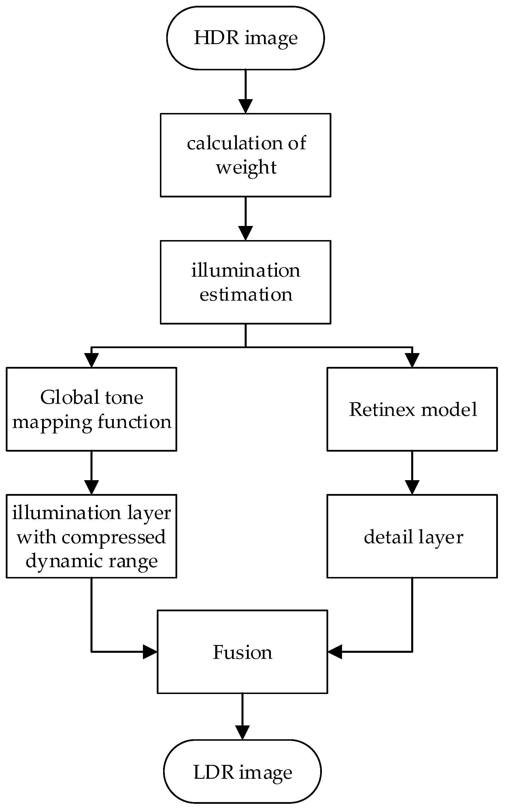
• The weight between the original image pixel points and other pixel points in their neighborhood is obtained by the least squares method, and the boundary-aware weights are introduced to prevent the halo artifacts and are used to estimate the illumination of the original image.
• The detail layer of the image is obtained by the Retinex model.
• A global tone mapping function with a parameter is used to process the illumination layer obtained in step (1).

After the above processing, the illumination layer and detail layer are fused to obtain the final LDR image.

3.1. The Illumination Estimation

We chose to obtain the weight of all pixel points in the image with their 3 × 3 neighborhood pixel points; each region includes nine pixels. Figure 2 shows the weight matrix of a pixel and its 3 × 3 neighborhood:

The luminance of any pixel is assumed to be weighted by the luminance of other pixels in the 3 × 3 neighborhood, and different pixel points correspond to the same weights as their neighborhoods. For all the different pixels, a function $f_k({\omega }_1,{\omega }_2,\dots ,{\omega }_9)$ is constructed concerning the 9-pixel weights, as shown in Equation (1).

$$f_{}({\omega }_1,{\omega }_2,\dots ,{\omega }_9)={\displaystyle \sum _{i=1}^H{{\displaystyle \sum _{j=1}^W{\left({\omega }_1{I}_{i-1,j-1}+{\omega }_2{I}_{i,j-1}+{\omega }_3{I}_{i+1,j-1}+\cdots +{\omega }_9{I}_{i+1,j+1}-I_{i,j}\right)}^2}}^{}}$$

(1)

where ${\omega }_1,{\omega }_2,\dots ,{\omega }_9$ is the weight of a pixel point with other pixels in its 3 × 3 neighborhood, $I_{i,j}$ denotes the brightness of a pixel with horizontal coordinate I and vertical coordinate j in the image pixel matrix, H is the image pixel matrix height value, and W is the width value of the image pixel matrix. According to the least squares criterion, the derivative function of any pixel weight ${\omega }_k$ of $f_{}$ is 0, i.e., Equation (2) holds.

$$\frac{\partial f({\omega }_1,{\omega }_2,\cdots ,{\omega }_9)}{\partial {\omega }_k}=0$$

(2)

Bringing all the weights into Equation (2) according to Equation (1), a linear system of equations on the pixel weights is obtained, as shown in Equation (3).

$$\{\begin{array}{l}{\displaystyle \sum _{i=1}^H{\displaystyle \sum _{j=1}^W\left({\omega }_1{I}_{i-1,j-1}+{\omega }_2{I}_{i,j-1}+\cdots +{\omega }_9{I}_{i+1,j+1}-I_{i-1,j-1}\right)\times I_{i-1,j-1}}}=0\\ {\displaystyle \sum _{i=1}^H{\displaystyle \sum _{j=1}^W\left({\omega }_1{I}_{i-1,j-1}+{\omega }_2{I}_{i,j-1}+\cdots +{\omega }_9{I}_{i+1,j+1}-I_{i,j-1}\right)\times I_{i,j-1}}}=0\\ \dots \\ {\displaystyle \sum _{i=1}^H{\displaystyle \sum _{j=1}^W\left({\omega }_1{I}_{i-1,j-1}+{\omega }_2{I}_{i,j-1}+\cdots +{\omega }_9{I}_{i+1,j+1}-I_{i+1,j+1}\right)\times I_{i+1,j+1}}}=0\end{array}$$

(3)

By solving Equation (3) through the Jacobi iteration method, the optimal solution of any pixel weight can be obtained, as shown in Equation (4):

$${\omega }_k^{(t)}=\frac{{\displaystyle \sum _{i=1}^H{\displaystyle \sum _{j=1}^W\left(I_{i,j}-\left({\omega }_1^{(t-1)}{I}_{i-1,j-1}+{\omega }_2^{(t-1)}{I}_{i,j-1}+\cdots +{\omega }_9^{(t-1)}{I}_{i+1,j+1}\right)\right)\times I_{i,j}}}}{{\displaystyle \sum _{i=1}^H{\displaystyle \sum _{j=1}^W{I}_{i,j}^2}}}-{\omega }_k^{(t-1)}$$

(4)

where $k\in [1,9]$, and the superscript t denotes the number of iterations. Let Equation (5) hold constant for all pixels. We set an error value to determine the termination of the iteration. When the error value is less than 0.001, the image effect difference does not change much. To take into account the efficiency and the image quality, we set the error value to 0.001.

$$\left|{\omega }_k^{(t)}-{\omega }_k^{t-1}\right|\le 0.001$$

(5)

Then, the Jacobi iterative method converges; at this point, ${\omega }_k^{(t)}$ is the least squares estimate of the pixel weights. The obtained weights are used to estimate the illumination. Equation (6) shows the estimation result of the illumination.

$$I_{(i,j)}^{*}={\omega }_1{I}_{i-1,j-1}+{\omega }_2{I}_{i,j-1}+{\omega }_3{I}_{i+1,j-1}+\cdots +{\omega }_9{I}_{i+1,j+1}$$

(6)

3.2. Improved Illumination Estimation

The experiment found that the difference between the brightness value of a pixel and other pixels in its neighborhood is too large, that is, if it is in the edge area, the artifact of a halo will occur. To prevent the artifact of halos, i.e., to achieve the function of edge detection, this paper introduces boundary-aware weights.

$$Z_G(I_{i,j}^{\prime })=N\times \frac{{\sigma }_G^2(I_{i,j}^{\prime })+\epsilon }{{\sigma }_G^2(I_{i,j}^{})+\epsilon }$$

(7)

where $i\in [1,H]$,$j\in [1,W]$, N is the total number of pixels in the $3\times 3$ area, ${\sigma }_G^2(I_{i,j}^{\prime })$ is the variance value of the pixel in the $3\times 3$ neighborhood window, and ${\sigma }_G^2(I_{i,j}^{})$ is the variance of all pixel points in the $3\times 3$ neighborhood except for the selected pixel points. As ${\sigma }_G^2(I_{i,j}^{})$ is the variance value whose minimal value can be 0 for the area where the luminance value remains unchanged, $\epsilon$ is a small constant value used to avoid the singularity that occurs with 0 values in these cases when taking division operation. It is used to ensure the validity of weights. We also should ensure that the value of $\epsilon$ is as small as possible while adapting to different images. So, when the input image is L, set it to ${(0.001L)}^2$. When $I_{i,j}^{\prime }$ is in the edge region, the value $Z_G(I_{i,j}^{\prime })$ is usually greater than 1. When $I_{i,j}^{\prime }$ is in the smoothing region, the value $Z_G(I_{i,j}^{\prime })$ is usually less than 1. We combined the interpixel weights obtained by the least squares method and obtained an improved illumination layer estimation for solving the halo artifacts, as shown in the following equation.

$$I_{i,j}^{*}={\omega }_1\frac{1}{Z_G(I_{i-1,j-1}^{\prime })}{I}_{i-1,j-1}+{\omega }_2\frac{1}{Z_G(I_{i,j-1}^{\prime })}{I}_{i,j-1}+\cdots +{\omega }_9\frac{1}{Z_G(I_{i+1,j+1}^{\prime })}{I}_{i+1,j+1}$$

(8)

where $I_{i,j}^{*}$ is the improved illumination estimation. When a pixel is at the edge, causing a large value of ${\omega }_j$, the introduction of boundary-aware weights can effectively reduce the impact of the brightness of other pixels, thus solving the halo artifacts caused by large differences in weights. When a pixel is in the smoothing region, introducing improved weights can enlarge the smoothing region and enhance the image details.

3.3. Dynamic Range Compression

To make full use of the advantages of histogram equalization and solve the problem of image over-enhancement caused by the method, in this paper, a global tone mapping function with a parameter was designed to compress the dynamic range. Based on the least squares, the parameter is calculated by fitting the global tone mapping function to the histogram equalization. The following equation is the global tone mapping function.

$$L_d(x,y)=\frac{I_{i,j}}{\alpha +I_{i,j}}$$

(9)

where $L_d(x,y)$ is the mapped luminance, $I_{i,j}$ is the input luminance value, and $\alpha$ is the parameter; the result of the mapping is shown in Figure 3.

We take the reciprocal of the global tone mapping function and histogram equalization results at the same time and build a functional relationship between the global tone mapping function and histogram equalization based on the least squares criterion:

$$F(\alpha )={\displaystyle \sum _{i=1}^H{\displaystyle \sum _{j=1}^W{\left[\frac{\alpha +I_{i,j}}{I_{i,j}}-\frac{1}{f(I_{i,j})}\right]}^2}}$$

(10)

where $f(I_{i,j})$ is the calculation result of histogram equalization. According to the least squares criterion, the derivative of $\alpha$ is 0; this shows that Equation (11) holds, and Equation (12) is obtained:

$$\frac{\partial F(\alpha )}{\partial \alpha }=0$$

(11)

$${\displaystyle \sum _{i=1}^H{\displaystyle \sum _{j=1}^W\left[\frac{(\alpha +I_{i,j})f(I_{i,j})-I_{i,j}}{I_{i,j}f(I_{i,j})}\right]=0}}$$

(12)

By solving Equation (12), the parameter $\alpha$ of the global tone mapping function can be obtained:

$$\alpha ={\displaystyle \sum _{i=1}^H{\displaystyle \sum _{j=1}^W\frac{I_{i,j}\left[1-f(I_{i,j})\right]}{f(I_{i,j})}}}$$

(13)

According to the obtained parameters, the global tone mapping functions corresponding to different images can thus be obtained, and the dynamic range compression of different images can be achieved.

3.4. LDR Image Generation

3.4.1. Detail Layer Estimation

The maximum value between each pixel RGB channel is set as the luminance component of the image, as shown in Equation (14).

$$L(x,y)=\max \left\{R(x,y),G(x,y),B(x,y)\right\}$$

(14)

where $L(x,y)$ is the luminance maximum for each pixel RGB channel, which is used to normalize the RGB colors. Then, calculate the color components for each channel, as shown in Equation (15).

$$r(x,y)=\frac{R(x,y)}{L(x,y)},g(x,y)=\frac{G(x,y)}{L(x,y)},b(x,y)=\frac{B(x,y)}{L(x,y)}$$

(15)

Based on the estimation of illumination obtained above, the detail layer of the image is obtained, as shown in the following equation

$$L^{*}(x,y)=\log (L(x,y))-\log (I_{i,j}^{*})$$

(16)

where $L^{*}(x,y)$ is the image detail layer.

3.4.2. Image Fusion and Color Retention

The detail layer and the illumination layer after dynamic range compression are fused to obtain the result, as shown in the following equation:

$$L_a(x,y)=\beta L_d(x,y)+\gamma {\mathrm{e}}^{L^{*}(x,y)}$$

(17)

where $L_a(x,y)$ is the brightness value after fusion, $\beta$ and $\gamma$ are the reconstruction coefficients of the image fusion process, and the reconstruction coefficients take different values because the image illumination layer and the detail layer contain different information. The illumination layer contains the dynamic range of the image, which generally needs to be compressed, and the choice for $\beta$ is generally less than 1. However, if the value is too small, it will cause problems such as a low overall brightness value and low contrast, which will affect the image quality. The detail layer contains the image detail information, which generally needs to be enhanced, and the choice $\gamma$ is generally greater than 1. However, it should not be set too large because it can cause excessive detail enhancement while creating problems such as halo artifacts and unnatural overall image effects. Based on that, we set $\beta$ and $\gamma$, respectively, to 0.8 and 1.2.

After the above processing, the color information needs to be recovered, as shown in the following equation.

$$\{\begin{array}{l}{R}^{*}(x,y)=L_a(x,y)\times {\left[r(x,y)\right]}^s\\ G^{*}(x,y)=L_a(x,y)\times {\left[g(x,y)\right]}^s\\ B^{*}(x,y)=L_a(x,y)\times {\left[b(x,y)\right]}^s\end{array}$$

(18)

where $R^{*}(x,y)$,$G^{*}(x,y)$,$B^{*}(x,y)$ are the three-channel information after color recovery, and s is the gamma correction factor that determines the color saturation of the recovered image. In most cases, we can achieve close-to-ideal colors mostly by using a monitor with a gamma value of 2.2. Most LCD monitors are designed based on a gamma value of 2.2. So, we set s = 1/2.2, i.e., s = 0.45, in our method.

4. Experimental Results and Analysis

An experimental platform with an Intel i5-6300HQ processor, 8 GB memory capacity, 64-bit Windows 10 operating system, and Matlab 2016b simulation software was used to verify the feasibility of the proposed method. The LDR images were displayed on a Samsung LCD monitor model S32AM700PC. HDR images from the TMQI database [14] were selected for experimental comparison and analysis, and all images in the TMQI database are shown in Figure 4. The dataset contains some high-dynamic range scenes from the world, such as landscape photos, architecture photos, etc. A total of 15 selected HDR images from the database were used to analyze and evaluate the LDR images tone-mapped by TVI-TMO [3], the method of Li et al. [7], the method of Aziz et al. [1], the method of Gu et al. [15], the method of Shibata et al. [16], and the proposed method. Tone-mapped images were evaluated by subjective and objective assessment.

4.1. Subjective Effect Analysis

The three sets of experimental results are shown in Figure 5, Figure 6, and Figure 7, respectively. From the experimental results, it can be seen that TVI-TMO retains the background information in the image, and the detail part is enhanced, but the overall brightness difference is large. The detail of the result of Li et al. is clearer, but the overall picture performance is not realistic. The result of Aziz et al. has good overall brightness performance, but there are incomplete details at extremely bright places. The result of Gu et al. is clear, but there is an artifact of the halo at the edge of the image. The result by Shibata et al. has overall good image perception, and the image details are clear, but there is the problem of low brightness. The proposed method has a good sense of image hierarchy, moderate brightness, and effectively preserves the edges of the original image and solves the halo artifacts, which is in line with the visual effect of the human eye.

Looking at Figure 6 and Figure 7, it can be seen that, when compared to the method of this paper, the method of Gu et al., although it seems clearer, is not universal. The evaluation of LDR images generated by the method of Gu et al. for different scenes is significantly different. Moreover, the method of Gu et al. suffers from halo artifacts, an unnatural appearance, color distortion, and overexaggerated detail. For example, the edge between the leaf and sky in Figure 6d shows clear halos, the detail of the trunk and the sunroof in Figure 5d and Figure 6d are overexaggerated, there are halo artifacts at the edges of the buildings and the sky in Figure 7d, and all three images produced by the method of Gu et al. suffer from low saturation. This demonstrates that the method of Gu et al. makes the output image visually unnatural to some extent.

We use the calculation of the mean opinion score (MOS) [7] for each comparison method to subjectively evaluate the tone mapping method. The method involves each participant in the experiment scoring each image on parameters such as brightness, contrast, and detail according to subjective visual effects. The method displayed the tone-mapped images on the monitor one by one. Eight experienced female and nine experienced male volunteers were selected, and each volunteer scored the images on the monitor subjectively in the range of [1,10]. The evaluation indexes include brightness, contrast, and detail. A rating of 1 represents the worst visual image, and a rating of 10 represents the best visual image. All the images in the TMQI database were scored, and the MOS values for each comparison method were counted. The obtained MOS score statistics are shown in Figure 8. The high values of the indicators in Figure 8 indicate that the image quality after tone mapping is good.

In the horizontal axis of Figure 8, the methods under comparison are displayed and the vertical coordinates are the MOS scores. The vertical line at the center of the upper boundary of the bar chart corresponds to the error line for each method, and the magnitude of the error line represents the standard deviation of the scores scored by different people.

Note that even though rare LDR images produced by the method of Gu et al. are cleaner than our method, the method of Gu et al. easily causes an unnatural effect by introducing halo artifacts, color distortion, and overexaggerated detail. More importantly, the method of Gu et al. is not a universal method. Thus, as an average evaluation, the MOS score of the image produced by the method of Gu et al. is a little lower than our method.

According to the scoring results, the results obtained by the proposed method were evaluated highly by most of the experimenters. The method has the smallest evaluation error, which indicates that the proposed method can adapt to the variability of images between different scenes, and the effect of the mapped images is consistent with the visual effect of most people and has strong stability for different individuals.

4.2. Objective Evaluation Effect Analysis

We used the objective evaluation method of tone mapping quality index (TMQI) [14] to evaluate the results of the method, after tone mapping, more comprehensively. The TMQI method consists of three evaluation metrics: structural fidelity, naturalness, and image quality score. Structural fidelity measures the extent to which the generated low-dynamic-range image maintains the structural information of the original image. Naturalness is a criterion designed by comparing the luminance statistics of a large number of natural images, and the larger the value, the more suitable it is for human eye observation. The image quality score is a composite score of the first two metrics. The TMQI scores are shown in

Table 1. Tone mapping TMQI scores.

Image Index	TVI-TMO	Li et al.	Aziz et al.	Gu et al.	Shibata et al.	Proposed Method
1	0.725	0.735	0.785	0.822	0.796	0.896
2	0.693	0.705	0.728	0.832	0.826	0.908
3	0.753	0.723	0.722	0.831	0.785	0.886
4	0.659	0.695	0.732	0.796	0.801	0.876
5	0.698	0.698	0.702	0.852	0.793	0.894
6	0.682	0.712	0.712	0.804	0.811	0.898
7	0.632	0.722	0.710	0.832	0.786	0.901
8	0.689	0.709	0.722	0.862	0.822	0.876
9	0.705	0.708	0.709	0.821	0.815	0.903
10	0.688	0.725	0.774	0.832	0.813	0.893
11	0.668	0.731	0.765	0.845	0.809	0.901
12	0.675	0.724	0.755	0.833	0.795	0.897
13	0.685	0.706	0.742	0.826	0.782	0.882
14	0.690	0.730	0.738	0.836	0.821	0.902
15	0.675	0.726	0.729	0.842	0.796	0.896
Average	0.687	0.720	0.734	0.831	0.803	0.893

.

In addition, the local mean Weber contrast (MLWC) [17] metric, natural image quality evaluator (NIQE) [18], and blind/referenceless image spatial quality evaluator (BRISQUE) [19] are selected to further evaluate the performance of each method. The mean local Weber contrast index is a perceived contrast measure based on Weber’s law, which takes into account the sensitivity of human visual effects to the spatial frequency content of an image. MLWC evaluates the image detail, and a higher the MLWC score indicates richer details of the LDR image. The natural image quality evaluator (NIQE) model extracts a set of local features from an image to evaluate image quality by using a multivariate Gaussian model. A smaller NIQE score indicates a higher image quality of the LDR image. BRISQUE compares the processed image to a default model computed from images of natural scenes with similar distortions. A small score indicates better perceptual quality. Several evaluation indexes’ scores are shown in

Table 2. Tone mapping MLWC and NIQE scores.

Image Index	TVI-TMO		Li et al.		Aziz et al.		Gu et al.		Shibata et al.		Proposed Method
	MLWC	NIQE	MLWC	NIQE	MLWC	NIQE	MLQC	NIQE	MLWC	NIQE	MLWC	NIQE
1	1.225	5.56	1.263	5.26	1.325	4.89	1.456	3.75	1.320	3.62	1.689	3.06
2	1.382	5.89	1.256	5.36	1.382	4.86	1.442	3.85	1.423	3.52	1.742	3.16
3	1.330	5.36	1.396	5.12	1.430	4.92	1.323	3.91	1.425	3.66	1.623	2.94
4	1.356	5.45	1.423	5.14	1.456	4.93	1.412	4.04	1.365	3.42	1.712	3.26
5	1.289	5.25	1.368	5.13	1.489	4.95	1.469	3.82	1.423	3.44	1.569	3.56
6	1.332	5.54	1.232	5.22	1.332	5.01	1.303	3.88	1.436	3.38	1.603	3.18
7	1.236	5.38	1.389	5.15	1.336	4.75	1.330	3.76	1.496	3.51	1.630	2.89
8	1.256	5.42	1.323	4.95	1.356	4.79	1.498	3.81	1.368	3.55	1.598	3.18
9	1.212	5.39	1.225	5.02	1.412	4.85	1.305	3.84	1.456	3.78	1.605	3.14
10	1.265	5.72	1.386	5.11	1.365	4.91	1.412	3.91	1.423	3.70	1.612	3.17
11	1.313	5.32	1.389	5.18	1.213	4.93	1.363	3.69	1.425	3.78	1.563	3.11
12	1.158	5.63	1.305	5.06	1.258	4.99	1.423	3.70	1.403	3.69	1.723	3.12
13	1.268	5.75	1.332	5.13	1.352	4.97	1.412	3.83	1.456	3.59	1.659	3.08
14	1.312	5.12	1.268	5.11	1.372	4.86	1.386	3.62	1.432	3.65	1.756	3.25
15	1.330	5.35	1.392	5.03	1.402	4.88	1.396	3.72	1.392	3.58	1.723	3.20
Mean	1.283	5.47	1.330	5.13	1.363	4.89	1.395	3.81	1.473	3.60	1.654	3.15

and

Table 3. Tone mapping BRISQUE scores.

Image Index	TVI-TMO	Li et al.	Aziz et al.	Gu et al.	Shibata et al.	Proposed Method
1	43.63	43.25	38.52	32.14	33.14	20.15
2	42.53	42.21	37.25	35.85	29.26	23.15
3	43.52	42.25	38.39	26.14	33.36	24.15
4	43.53	43.25	35.26	31.25	34.57	21.14
5	42.25	42.38	39.25	30.25	38.14	20.19
6	40.59	43.12	37.32	29.25	35.25	22.83
7	41.28	42.24	36.25	32.18	33.14	20.69
8	38.58	42.69	38.25	30.15	33.47	20.73
9	42.55	44.89	36.14	33.25	32.16	22.14
10	43.52	42.28	35.69	30.19	32.47	22.98
11	44.25	42.12	35.89	28.93	33.88	20.78
12	43.52	43.25	37.25	34.12	34.17	22.79
13	42.36	42.25	37.86	30.13	33.49	21.47
14	43.14	41.25	36.14	31.25	32.95	20.83
15	43.25	42.25	39.25	26.85	31.85	19.09
Mean	42.57	42.65	37.25	30.80	33.42	21.54

.

As can be seen from Table 1, the TMQI score of this method is higher than other methods, which indicates that the proposed method maintains a better structure and the visual effect is closer to the real scene. From Table 2, the MLWC score is higher than other methods, which indicates that the proposed method is better than other methods in terms of detail richness. The NIQE and BRISQUE scores are lower than those of several other methods, which indicates that the proposed method is better than other methods in terms of image quality.

5. Conclusions

In this paper, we proposed a tone mapping method based on the least squares. Our purpose is to reveal the local contrast of real-world scenes on a conventional monitor. Based on the classical Retinex model, we used the interimage weights by the least squares for illumination estimation, while we introduced boundary-aware weights to prevent halo artifacts. The detail layer is obtained by the above method. The method using weights takes into account the luminance intensity and pixel position, which can prevent the generation of halo artifacts while ensuring accurate estimation of illumination information. A global tone mapping function with the parameter is applied to the obtained illumination estimation to compress the dynamic range. The function is obtained by fitting the histogram equalization results, and different images correspond to different parameter values. This method can achieve dynamic range compression for different images more effectively. The detail layer and the illumination layer after dynamic range compression are fused to obtain the LDR image. The high dynamic range scenes in the TMQI dataset were selected for comparative analysis from both subjective and objective aspects. The experimental results show that details of both dark and highlighted regions are preserved, and halo artifacts do not appear. In the proposed method, the TMQI score of LDR images is 0.893 and the MLWC score is 1.654; the detail richness, structure fidelity, and visual effect are all better than other methods in different degrees. In this paper, we focused on solving the problems of illumination estimation and dynamic range compression in tone mapping, and we will focus on using tone mapping for video processing in the future.

References

1. Khan, I.R.; Aziz, W.; Shim, S.O. Tone Mapping Using Perceptual-quantizer and Image Histogram. IEEE Access 2020, 12, 12–15. [Google Scholar] [CrossRef]
2. Choi, H.H.; Kang, H.S.; Yun, B.J. A Perceptual Tone Mapping HDR Images Using Tone Mapping Operator and Chromatic Adaptation Transform. Imaging Sci. Technol. 2017, 61, 15–20. [Google Scholar] [CrossRef]
3. Khan, I.R.; Rahardja, S.; Khan, M.M.; Movania, M.M.; Abed, F.A. Tone Mapping Technique Based on Histogram Using a Sensitivity Model of The Human Visual System. IEEE Trans. Ind. Electron. 2018, 65, 3469–3479. [Google Scholar] [CrossRef]
4. Husseis, A.; Mokraoui, A.; Matei, B. Revisited Histogram Equalization as HDR Images Tone Mapping Operators. IEEE Comput. Soc. 2017, 15, 144–149. [Google Scholar]
5. Chien, B.; Mokraoui, A.; Matei, B. Contrast Enhancement and Details Preservation of Tone Mapped High Dynamic Range Images. Image Represent. 2018, 58, 22–26. [Google Scholar]
6. Kai-Fu, Y.; Hui, L.; Hulin, K.; Chao-Yi, L.; Yong-Jie, L. An Adaptive Method for Image Dynamic Range Adjustment. IEEE Trans. Circuits Syst. Video Technol. 2019, 29, 15–18. [Google Scholar]
7. Hui, L.; Xixi, J.; Zhang, L. Clustering Based Content and Color Adaptive Tone Mapping. Comput. Vis. Image Underst. 2018, 168, 15–20. [Google Scholar]
8. Thai, B.C.; Mokraoui, A. HDR Image Tone Mapping Histogram Adjustment with Using an Optimized Contrast Parameter. In Proceedings of the International Symposium on Signal, Image, Video and Communications (ISIVC), Rabat, Morocco, 27–30 November 2018; Volume 12, pp. 15–20. [Google Scholar]
9. Fahim, M.A.N.I.; Jung, H.Y. Fast Single-Image HDR Tone Mapping by Avoiding Base Layer Extraction. Sensors 2020, 20, 4378. [Google Scholar] [CrossRef] [PubMed]
10. Gommelet, D.; Roumy, A.; Guillemot, C.; Ropert, M.; Julien, L. Gradient-Based Tone Mapping for Rate-Distortion Optimized Backward-Compatible High Dynamic Range Compression. IEEE Trans. Image Processing 2017, 15, 12–18. [Google Scholar] [CrossRef] [PubMed]
11. Liang, Z.; Xu, J.; Zhang, D. A Hybrid l1-l0 layer Decomposition Model for Tone Mapping. In Proceedings of the IEEE Conference on Computer Vision and Pattern Recognition, Salt Lake City, UT, USA, 18–23 June 2018; pp. 4758–4766. [Google Scholar]
12. Rana, A.; Singh, P.; Valenzise, G.; Dufaux, F.; Komodakis, N.; Smolic, A. Deep Tone Mapping Operator for High Dynamic Range Images. IEEE Trans. Image Processing 2019, 29, 18–25. [Google Scholar] [CrossRef] [PubMed] [Green Version]
13. Hu, L.; Chen, H.; Allebach, J.P. Joint Multi-Scale Tone Mapping and Denoising for HDR Image Enhancement. In Proceedings of the IEEE/CVF Winter Conference on Applications of Computer Vision, Waikoloa, HI, USA, 3–8 January 2022; Volume 26, pp. 729–738. [Google Scholar]
14. Yeganeh, H.; Wang, Z. Objective Quality Assessment of Tone-mapped Images. IEEE Trans. Image Processing 2012, 22, 657–667. [Google Scholar] [CrossRef] [PubMed]
15. Gu, B.; Li, W.; Zhu, M. Local Edge-preserving Multiscale Decomposition for High Dynamic Range Image Tone Mapping. IEEE Trans. Image Processing 2012, 22, 70–79. [Google Scholar]
16. Shibata, T.; Tanaka, M. Gradient-domain Image Reconstruction Framework with Intensity-range and Base-structure Constraints. In Proceedings of the IEEE Conference on Computer Vision and Pattern Recognition, Las Vegas, NV, USA, 27 June 2016; pp. 2745–2753. [Google Scholar]
17. Khosravy, M.; Gupta, N.; Marina, N. Perceptual Adaptation of Image Based on Chevreul–Mach Bands Visual Phenomenon. IEEE Signal Processing Lett. 2017, 24, 594–598. [Google Scholar] [CrossRef]
18. Mittal, A.; Soundararajan, R.; Bovik, A.C. Making a “completely blind” image quality analyzer. IEEE Signal Process. Lett. 2012, 20, 209–212. [Google Scholar] [CrossRef]
19. Mittal, A.; Moorthy, A.K.; Bovik, A.C. No-reference image quality assessment in the spatial domain. IEEE Trans. Image Process. 2012, 21, 4695–4708. [Google Scholar] [CrossRef] [PubMed]
Figure 1. Flow chart of the method in this paper.
Electronics 12 00031 g001
Figure 2. Pixel matrix in the 3 × 3 neighborhood.
Electronics 12 00031 g002
Figure 3. The dynamic range compression curve.
Electronics 12 00031 g003
Figure 4. TMQI dataset.
Electronics 12 00031 g004
Figure 5. The tone-mapped images of the church. (a) Result of TVI-TMO; (b) Result of Li et al.; (c) result of Aziz et al.; (d) result of Gu et al.; (e) result of Shibata et al.; (f) result of the proposed method.
Electronics 12 00031 g005aElectronics 12 00031 g005b
Figure 6. The tone-mapped images of the landscape. (a) Result of TVI-TMO; (b) result of Li et al.; (c) result of Aziz et al.; (d) result of Gu et al.; (e) result of Shibata et al.; (f) result of the proposed method.
Electronics 12 00031 g006aElectronics 12 00031 g006b
Figure 7. The tone-mapped images of the architecture. (a) Result of TVI-TMO; (b) result of Li et al.; (c) result of Aziz et al.; (d) result of Gu et al.; (e) result of Shibata et al.; (f) result of the proposed method.
Electronics 12 00031 g007
Figure 8. Statistical chart of MOS scores.
Electronics 12 00031 g008