Calculation and Analysis of Characteristic Parameters for Lossy Resonator

Abstract

Resonator is widely employed in microwave and millimeter-wave fields. However, it is challenging and crucial to calculate the electromagnetic field distribution in the resonant cavity with various loss dielectrics. In this paper, according to the axisymmetric distribution characteristics of the lossy resonator, the electromagnetic function of each part in the cavity is established with the Borgnis function, the characteristic equation is obtained based on the mode-matching method, and the resonance frequency and Q factor of the eigenmode TM₀₁₀ are numerically calculated. With the proposed method, the impact of various dielectric structures and characteristics parameters on the resonant properties of the TM₀₁₀ mode may be thoroughly examined by taking into account the influence of the thickness as well as the materials of the lossy layer in the z direction. The relative error between the theoretical and the simulated results is below 0.7% at different structures and lossy dielectrics, which indicates that the general calculation approach, as well as crucial data and structure references, is suitable for a related device design in TM₀₁₀ mode.

1. Introduction

One of the frontiers of international research since the turn of the twenty-first century is the study and use of microwave and millimeter-wave technology [1]. There are several applications and growth opportunities for various types of microwave equipment in contemporary military electronic countermeasures, hyper-firing-rate weapon development, microwave heating, etc. The performance of many microwave devices is greatly influenced by the resonant properties of microwave resonators [2]. To optimize the performance of devices, it is necessary to calculate and analyze the electromagnetic field distribution in the resonant cavity and comprehend the impact of different structural parameters on the resonant characteristics. By this approach, it can provide a thorough theoretical foundation and useful structural guidelines.

There are infinite operating modes when the electromagnetic field is stimulated in the resonant cavity, and interferences between the nearby resonant modes can impact the device’s stability [3]. To prevent further high-order modes and ensure the device’s functionality, lossy dielectrics must be coated in the resonant cavity. Additionally, the use of a relative structure is still up for debate in several microwave-technology-related fields, including microwave heating [4,5], microwave attenuation materials [6,7,8], and atom frequency standards [9,10].

Numerous studies on pertinent topics have recently been conducted. In the rubidium frequency standard, Qian Huang et al. introduced a particular type of microwave cavity filled with a complex structure dielectric and examined this structure using the mode-matching method and a CST simulation [11]. The matching procedure in this method, however, was more centered on the r direction, and the sole characteristic parameter that was calculated was the resonant frequency; the Q factor was not taken into account. By using the finite element approach, Liaoyuan Song et al. developed a microwave-heated device and studied the electromagnetic field within its resonant cavity [12,13,14]. However, this method was simulation-heavy with little mathematical analysis, and it focused primarily on the TE mode in rectangular cavities.

Kanthal coating made by selective laser melting was studied for its microstructure and microwave attenuation capabilities by Yongqing Zhang et al [15]. A CST simulation was used to verify the performance of a newly built microwave attenuation layer with magnetic dissipation [15]. The study did not, however, provide many physical mechanisms. The electromagnetic wave propagation in a lossy cylindrical waveguide was covered by Jirun Luo et al. [16]. By roughly estimating several parameters, the dispersion equations were made simpler, and the computation results were accurate enough that the error was less than 3%. When used to address cavity resonant difficulties, this type of approximation method offers a typical solution to challenging electromagnetic problems, but its accuracy and efficacy need to be further investigated.

One accurate measurement of microwave permittivity based on electromagnetic fields in a cavity resonator with finite conductivity walls was proposed by Hiroyuki Tanaka et al. [17,18,19,20]. A metal-shelled form with a center dielectric rod was under discussion. Both the resonance frequency and Q factor of the higher-order mode calculations were also verified for accuracy. The study placed more emphasis on the center rod’s influence and the consideration of metal loss; this was highly precise but difficult to accomplish at the same time. Additionally, the absence of lossy dielectric layers around the cavities in the model may have had an impact on resonant properties.

In light of the aforementioned circumstances, this study suggests a typical cylindrical lossy resonator model and performs the analysis of the TM₀₁₀ mode field distribution in the lossy resonator using the Borgnis function [21] and the mode-matching method [21,22,23].

The Borgnis function is very convenient when there are two functions named as U and V in an orthogonal curvilinear coordinate system, which possess a definite relationship with all electromagnetic field components. In a cylindrical coordinate system, U and V further satisfy the Helmholtz equation. Consequently, it is simple to acquire the specific representations of U and V according to Equations (A1)–(A6) of Appendix A.

Then, according to the mode-matching method, each field component can be expanded into a certain progression where each of them represents a specific mode, respectively, and the tangential field components at the interface of the dielectric are equal. As a result, a matrix containing characteristic parameters is obtained. In this paper, the matching process is operated at surface z = h₁ and z = −h₁.

Finally, the resonant frequency and quality factor are numerically calculated using a computer program based on the secant method [24,25]. The main idea is that we first set two appropriate initial frequency values to start the calculation. After that, the wave number of each mode in all regions is calculated at the corresponding frequency. Ultimately, all the parameters are substituted into the matrix acquired by the mode-matching method so that the determinants are calculated for the two conditions. If the difference coefficient is within the tolerance, the resonant frequency is determined. It is believed that this calculation method is reliable because the resonant frequency of a normal mode cannot be null so that the convergence can be absolutely achieved. The basic iteration function is shown in Appendix B as Equation (A7).

The results of the computation are contrasted with the CST simulation. In the 2.5 GHz to 3.7 GHz range, the impact of various dielectric structures and losses on the resonant properties of TM₀₁₀ mode is thoroughly examined. The findings demonstrate that the approach is accurate and stable and that it can be applied generically to the calculation and analyses of such structures.

2. Calculation and Analysis Model

The general cylindrical lossy resonator calculation model proposed in this paper is shown in Figure 1 in the form of a sectional drawing. The longitudinal section and transverse section illustrate that the outermost layer of the cylindrical lossy resonator was considered as a “perfect conducting wall” (PCW) for the calculation. Region 1 was defined as an area full of one dielectric with a specific permittivity. Regions 2 and 3 were the cap-shaped lossy dielectrics coated at both ends of the cavity. The length of the entire resonator was slightly less than its diameter, which meant that the resonator was flat, and it determined that the first operating mode was the TM₀₁₀ mode [21].

The general steps for obtaining the solution of characteristic parameters were as follows:

• Developing electromagnetic field expressions and dividing regions. The electromagnetic field components of each zone in the entire model were determined by the Borgnis function, which was separated into numerous regular portions;
• Acquiring characteristic equations. By using the mode-matching method, some equations were created at the interface between various dielectrics;
• Numerical simulation. This process used the secant method to numerically solve for the resonant frequency and Q value, which can result in rapid convergence.

2.1. Establishment of Electromagnetic Field Components in Each Region

As shown in Figure 1, the radius of the resonator was r₁ and the length was 2 h₂. The thickness of the cap-shaped dielectric coated longitudinally was h₂ − h₁, and the whole structure was symmetric about the z-axis. The calculation model was divided into 3 regions. Region 1 was regarded as a vacuum with ε₀ permittivity, region 2 and region 3 were cap-shaped lossy dielectric coated on both ends of the cavity, respectively, and the corresponding permittivities were ε₂ and ε₃. Moreover, the relative permeability of all regions equaled 1.

At first, area 1 was considered as a typical circular waveguide [26] and regions 2 and 3 were regarded as circular waveguides filled with a lossy dielectric. For a specific mode, the change of electric field and magnetic field in the ϕ direction should be the same for all 3 regions. Since the TM_0i mode was even in the ϕ direction [27], it could be obtained that the field component in the ϕ direction equaled 1. In addition, the PCW was set at the outermost layer (surface at r = r₁, r = −r₁, z = h₂, and z = −h₂) for the numerical computation. Thus, the z-direction component of the U function in region 2 and region 3 could be written as a hyperbolic cosine function to meet the boundary conditions, while the component in region 1 was the superposition of forward and backward waves. Moreover, the ratio of the resonator length to the radius was maintained at 0.7, which meant the first mode of the cavity was the TM mode. In summary, according to the Borgnis function, the V function was 0 and the U function of each region could be described as follows:

For region 1:

$$U_{mid}={\displaystyle \sum }_{i=1}^{\infty }{J}_0\left(k_{ci}^{\left(n\right)}r\right)·\left(A_i{e}^{-{\gamma }_i^{\left(n\right)}z}+B_i{e}^{{\gamma }_i^{\left(n\right)}z}\right)$$

(1)

For region 2:

$$U_{up}={\displaystyle \sum }_{j=1}^{\infty }{a}_j·J_0\left(k_{cj}^{\left(n\right)}r\right)·\cosh {\gamma }_j^{\left(n\right)}\left(h_2-z\right)$$

(2)

For region 3:

$$U_{bot}={\displaystyle \sum }_{j=1}^{\infty }{b}_j·J_0\left(k_{cj}^{\left(n\right)}r\right)·\cosh {\gamma }_j^{\left(n\right)}\left(h_2+z\right)$$

(3)

where $k_{ci}^{\left(n\right)}$ and ${\gamma }_i^{\left(n\right)}$ are propagation constants of the ith mode in the region of n in the r direction and z direction, respectively, $A_i$ and $B_i$ are the amplitude of the forward wave and backward wave for the ith mode, respectively, and $a_j$ and $b_j$ are unknown constants of the jth mode which depend on boundary conditions. $J_0\left(k_{ci}^{\left(n\right)}r\right)$ are Bessel functions of the first kind [28] of order 0 and $J_0^{\prime }\left(k_{ci}^{\left(n\right)}r\right)$ is its derivative.

The electromagnetic field components of each region may therefore be described as follows using Equations (1)–(3) and the relationship between the U and V functions and the field components according to Appendix A:

For region 1:

$$E_{ri}^{\left(n\right)}={\displaystyle \sum }_{i=1}^{\infty }-k_{ci}^{\left(n\right)}{\gamma }_i^{\left(n\right)}·J_0^{\prime }\left(k_{ci}^{\left(n\right)}r\right)·\left(A{e}^{-{\gamma }_i^{\left(n\right)}z}-B{e}^{{\gamma }_i^{\left(n\right)}z}\right)$$

(4)

$$E_{zi}^{\left(n\right)}={\displaystyle \sum }_{i=1}^{\infty }{k}_{ci}^{\left(n\right)}{}^2·J_0\left(k_{ci}^{\left(n\right)}r\right)·\left(A{e}^{-{\gamma }_i^{\left(n\right)}z}+B{e}^{{\gamma }_i^{\left(n\right)}z}\right)$$

(5)

$$H_{\varphi i}^{\left(n\right)}={\displaystyle \sum }_{i=1}^{\infty }-j\omega {\epsilon }_n{k}_{ci}^{\left(n\right)}·J_0^{\prime }\left(k_{ci}^{\left(n\right)}r\right)·\left(A{e}^{-{\gamma }_i^{\left(n\right)}z}+B{e}^{{\gamma }_i^{\left(n\right)}z}\right)$$

(6)

$$H_{zi}=H_{ri}=E_{\varphi i}=0$$

(7)

For region 2:

$$E_{rj}^{\left(n\right)}={\displaystyle \sum }_{j=1}^{\infty }{a}_j·\left[-k_{cj}^{\left(n\right)}{\gamma }_j^{\left(n\right)}·J_0^{\prime }\left(k_{cj}^{\left(n\right)}r\right)\right]·\sinh {\gamma }_j^{\left(n\right)}\left(h_2-z\right)$$

(8)

$$E_{zj}^{\left(n\right)}={\displaystyle \sum }_{j=1}^{\infty }{a}_j·k_{cj}^{\left(n\right)}{}^2·J_0\left(k_{cj}^{\left(n\right)}r\right)·\cosh {\gamma }_j^{\left(n\right)}\left(h_2-z\right)$$

(9)

$$H_{\varphi j}^{\left(n\right)}={\displaystyle \sum }_{j=1}^{\infty }{a}_j·\left[-j\omega {\epsilon }_n{k}_{cj}^{\left(n\right)}·J_0^{\prime }\left(k_{cj}^{\left(n\right)}r\right)\right]·\cosh {\gamma }_j^{\left(n\right)}\left(h_2-z\right)$$

(10)

$$H_{zj}=H_{rj}=E_{\varphi j}=0$$

(11)

For region 3:

$$E_{rj}^{\left(n\right)}={\displaystyle \sum }_{j=1}^{\infty }{b}_j·\left[k_{cj}^{\left(n\right)}{\gamma }_j^{\left(n\right)}·J_0^{\prime }\left(k_{cj}^{\left(n\right)}r\right)\right]·\sinh {\gamma }_j^{\left(n\right)}\left(h_2+z\right)$$

(12)

$$E_{zj}^{\left(n\right)}={\displaystyle \sum }_{j=1}^{\infty }{b}_j·k_{cj}^{\left(n\right)}{}^2·J_0\left(k_{cj}^{\left(n\right)}r\right)·\cosh {\gamma }_j^{\left(n\right)}\left(h_2+z\right)$$

(13)

$$H_{\varphi j}^{\left(n\right)}={\displaystyle \sum }_{j=1}^{\infty }{b}_j·\left[-j\omega {\epsilon }_n{k}_{cj}^{\left(n\right)}·J_0^{\prime }\left(k_{cj}^{\left(n\right)}r\right)\right]·\cosh {\gamma }_j^{\left(n\right)}\left(h_2+z\right)$$

(14)

$$H_{zj}=H_{rj}=E_{\varphi j}=0$$

(15)

where $\omega$ is the complex angular frequency and it equals $2\pi f_r\left(1+j/2Q_0\right)$, $f_r$ is the resonant frequency, $Q_0$ is the unloaded Q-factor of the resonance. ${\epsilon }_n$ represents the complex permittivity of region n and it equals ${\epsilon }_{rn}{\epsilon }_0\left(1-j\tan \delta \right)$, wherein ${\epsilon }_{rn}$ is the relative permittivity of region n and $\delta$ is the loss angle of the dielectric.

2.2. Boundary Conditions and Characteristic Equations

For region 1, the tangential components of the electric field and magnetic field should be 0 at r = r₁ [29]. Thus, Equation (16) could be obtained using the above conditions as well as Equations (4)–(7). Meanwhile, the relationship between $k_{ci}^{\left(1\right)}$ and ${\gamma }_i^{\left(1\right)}$ was defined as Equation (17).

Once an appropriate frequency was given, the values of $k_{ci}^{\left(n\right)}$ and ${\gamma }_i^{\left(n\right)}$ could be obtained by solving Equations (16) and (17) simultaneously. Similarly, for region 2 and 3, the tangential components possessed identical boundary conditions as those of region 1. Consequently, with Equations (8)–(15), the relation between $k_{cj}^{\left(n\right)}$ and ${\gamma }_j^{\left(n\right)}$ for n = 2 and 3 could be acquired. In conclusion, $k_{cj}^{\left(n\right)}$ and ${\gamma }_j^{\left(n\right)}$ for all regions were obtained by solving the following same equations.

$$J_0\left(k_{cj}^{\left(n\right)}r\right)=0$$

(16)

$$k_{cj}^{\left(n\right)}{}^2={\omega }^2{\mu }_0{\epsilon }_n+{\gamma }_j^{\left(n\right)}{}^2$$

(17)

The other boundary conditions that the tangential components of the electric field and magnetic field needed to satisfy could be obtained at z = h₂ and z = −h₂, and they could be described as follows for n = 1.

$$E_{rj}^{\left(2\right)}{|}_{z=h_1}=E_{ri}^{\left(1\right)}{|}_{z=h_1}$$

(18)

$$H_{\varphi j}^{\left(2\right)}{|}_{z=h_1}=H_{\varphi i}^{\left(1\right)}{|}_{z=h_1}$$

(19)

$$E_{rj}^{\left(3\right)}{|}_{z=-h_1}=E_{ri}^{\left(1\right)}{|}_{z=-h_1}$$

(20)

$$H_{\varphi j}^{\left(3\right)}{|}_{z=-h_1}=H_{\varphi i}^{\left(1\right)}{|}_{z=-h_1}$$

(21)

Then, the self-orthogonality [30] of the Bessel function was used to integrate over the transverse cross section of the boundary based on the products of Equations (18)–(21), allowing the unnecessary variables to be removed. Finally, the following characteristic matrix was obtained at the conditions of ${\epsilon }_2={\epsilon }_3$.

$$\begin{array}{c}{\displaystyle {\displaystyle \sum }_{i=1}^{\infty }}{\displaystyle {\displaystyle \sum }_{j=1}^{\infty }}(X_{ji}{A}_i+Y_{ji}{B}_i)=0\end{array}$$

(22)

$${\displaystyle \sum }_{i=1}^{\infty }{\displaystyle \sum }_{j=1}^{\infty }\left(Y_{ji}{A}_i+X_{ji}{B}_i\right)=0$$

(23)

Therein,

$$X_{ji}=e^{-{\gamma }_i^{\left(1\right)}{h}_1}\left[\sinh {\gamma }_j^{\left(2\right)}\left(h_2-h_1\right)·\oint H_{ji}dS-\cosh {\gamma }_j^{\left(2\right)}\left(h_2-h_1\right)·\oint E_{ji}dS\right]$$

(24)

$$Y_{ji}=e^{{\gamma }_i^{\left(1\right)}{h}_1}\left[\sinh {\gamma }_j^{\left(2\right)}\left(h_2-h_1\right)·\oint H_{ji}dS+\cosh {\gamma }_j^{\left(2\right)}\left(h_2-h_1\right)·\oint E_{ji}dS\right]$$

(25)

$$\oint E_{ji}dS={{\displaystyle \int }}_0^{r_2}\frac{k_{ci}^{\left(1\right)}{\gamma }_i^{\left(1\right)}}{k_{cj}^{\left(2\right)}{\gamma }_j^{\left(2\right)}}·J_0^{\prime }\left(k_{cj}^{\left(2\right)}r\right)J_0^{\prime }\left(k_{ci}^{\left(1\right)}r\right)rdr$$

(26)

$$\oint H_{ji}dS={{\displaystyle \int }}_0^{r_2}\frac{k_{ci}^{\left(1\right)}{\epsilon }_1}{k_{cj}^{\left(2\right)}{\epsilon }_2}·J_0^{\prime }\left(k_{cj}^{\left(2\right)}r\right)J_0^{\prime }\left(k_{ci}^{\left(1\right)}r\right)rdr$$

(27)

The resonant frequency corresponds to the real part of the root of the following equation, and $Q_0$ can be calculated from the imaginary part.

$$\left|\begin{array}{cc}X& Y\\ Y& X\end{array}\right|=0$$

(28)

The starting order of Equation (28) is infinite. In practice, it is truncated at a predetermined number of normal modes. In this study, there were 5 normal modes used in the calculation.

2.3. The Solution Method of Characteristic Equations

The secant method was used to calculate the characteristic parameters.

Figure 2 shows a flow chart of the calculation based on the secant method. After all the construction parameters are ready, the loop is started. Then, $k_{ci}^{\left(n\right)}$, ${\gamma }_i^{\left(n\right)}$, $k_{cj}^{\left(n\right)}$ and ${\gamma }_j^{\left(n\right)}$ for each mode are calculated corresponding to two frequencies, respectively. The values for Equation (28) are discovered, and they are given the names mat_H and mat_L. When the mat_H fails to fulfill the accuracy standard, we compute the difference coefficient, abbreviated diff. At the same time, a new iteration value, abbreviated f_new, is generated, and the loop is restarted. The convergence requirement is met and the final numerical results are achieved if mat_H is less than the tolerance. In this paper, the tolerance equaled 10⁻⁶.

3. Numerical Calculation Results and Analysis of the Influence of Dielectric Structure on Resonance Characteristics

In this part, the contents focus on the influence of the structure parameters of the cap-shaped dielectric on the resonant characteristics, including the thickness of the dielectric and different dielectric losses. All tests are carried out while other variables remain unchanged. The calculation accuracy is well checked by the comparison between the results of the computer program and the CST simulation. Moreover, various physical mechanisms causing the change of characteristic parameters are discussed in detail.

3.1. Analysis of the Influence of Dielectric Thickness on Resonance Characteristics

First, the thickness variation of the cap-shaped dielectric was thoroughly studied to analyze how the coated dielectric parameters affected the resonant properties. The loss of metal was not taken into account.

Table 1. The calculation results of resonant frequency for TM₀₁₀ mode changing with dielectric thickness compared with CST simulation.

delta h/mm	frc/GHz	frs/GHz	Error
1.0	3.6661	3.6651	0.027%
1.5	3.5672	3.5661	0.031%
2.0	3.4600	3.4588	0.035%
2.5	3.3443	3.3429	0.042%
3.0	3.2206	3.2189	0.053%
3.5	3.0905	3.0889	0.052%
4.0	2.9562	2.9544	0.061%
4.5	2.8201	2.8186	0.053%
5.0	2.6846	2.6825	0.078%
5.5	2.5514	2.5496	0.071%

and

Table 2. The calculation results of Q₀ for TM₀₁₀ mode changing with dielectric thickness compared with CST simulation.

delta h/mm	Q0c	Q0s	Error
1.0	31,460	31,264	0.627%
1.5	16,295	16,215	0.493%
2.0	9448	9418	0.319%
2.5	5938	5925	0.219%
3.0	3997	3990	0.175%
3.5	2862	2861	0.035%
4.0	2169	2167	0.092%
4.5	1724	1726	0.116%
5.0	1432	1434	0.139%
5.5	1233	1235	0.162%

tabulate the calculated results for the characteristic parameters compared with those of the CST simulation. In this section, r₁ = 29.85 mm, 2 h₂/r₁ = 0.7, ε_r2 = ε_r3 = 11.4, tan δ₂ = tan δ₃ = 0.0027. In the tables, delta h represents the thickness of the lossy dielectric in the z direction. f_rc and Q_0c are numerical calculation results while f_rs and Q_0s are simulation results. The assumption was that the first five terms of the electromagnetic field equations represented the Bessel function series in all calculations. The results demonstrated that the proposed method for determining the resonant frequency and unloaded Q value was accurate under these circumstances. The error of the resonant frequency calculation was within 0.1% and it was within 0.7% for the Q₀ value calculation. On the other hand, it can be concluded that the resonant frequency and unloaded Q factor of the TM₀₁₀ mode decreased significantly with the increase of the thickness. The former decreased by about 1.12 GHz and the latter was reduced by about 30,000 when the thickness reached 5.5 mm.

As shown in Figure 3, with the increase of the dielectric thickness in the z direction, the resonant frequency of the TM₀₁₀ mode tended to decrease linearly. For every 0.5 mm increment of the cap-shaped dielectric thickness, the value of f_r reduced by about 0.11 GHz. This was because the TM₀₁₀ mode had a strong longitudinal electric field in the axial region of the resonator. As a result, when the lossy dielectric coating was too thick in the longitudinal direction, it absorbed the energy of the electric field, increasing the loss of the resonant cavity and lowering the resonant frequency of the mode. Meanwhile, the increase of the dielectric thickness in the z direction meant that the dielectrics at both ends were closer, which may have led to the increase of equivalent capacitance of the cavity. This phenomenon can also cause the reduction of f_r. Thus, the position of the lossy dielectric in the z-direction has a significant impact on f_r. It is also important to keep in mind that the accuracy significantly decreased when the cap-shaped dielectric was quite thick, even though the overall calculation results were still very precise. However, when the dielectric was thin, the equivalent capacitance of the cavity was small and the simulation process might be less influenced by it, so that the error of the former was smaller.

Figure 4 illustrates the variation trend of the Q factor with the increase of the dielectric thickness in the z direction. When the thickness increased, Q factor dropped significantly between 1 and 3 mm. In addition, the inaccuracy tended to be less noticeable in dense situations. The loss increased as the longitudinal dielectric came closer to the cavity’s core section. This phenomenon can be attributed to the fact that the electric field energy of the TM₀₁₀ mode in this cavity was primarily concentrated in the central axis area [31], which is directly shown in Figure 5. Meanwhile, a thin dielectric meant a small loss, and the simulation process might ignore the loss from the area of weak electric activity. Therefore, the error of the latter was larger. Similarly, the conclusion would be opposite in a thick dielectric situation.

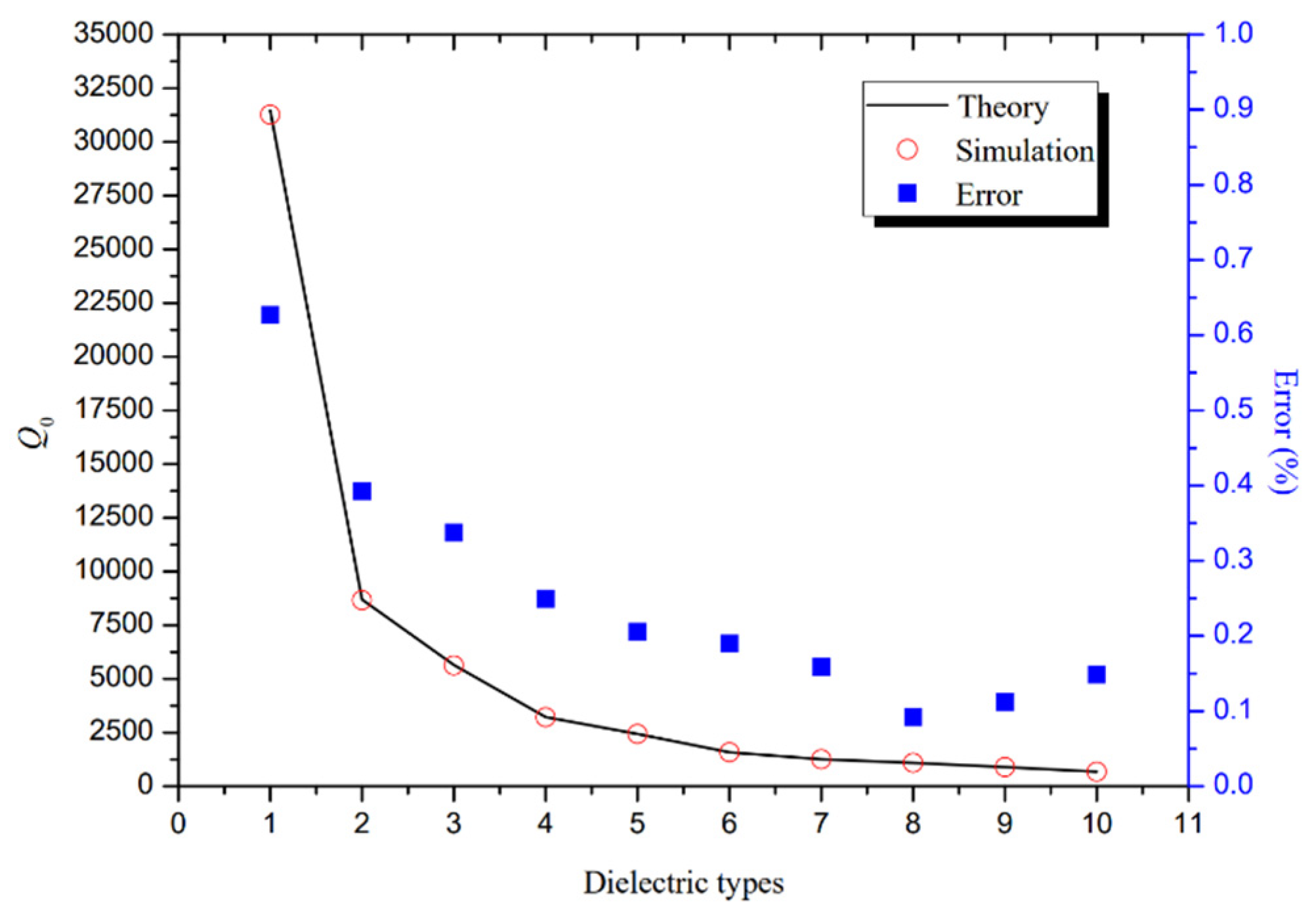
3.2. Analysis of the Influence of Dielectric Loss on Resonance Characteristics

In this section, the accuracy of the calculation and the impact on the resonant characteristic of various dielectric losses are examined. We could infer from part A that an increase in the thickness of lossy dielectrics in the z direction would result in energy dissipation, which could significantly affect the cavity’s resonance frequency and Q value for the TM₀₁₀ mode. Consequently, we chose 10 different kinds of lossy dielectrics and studied how they would affect the characteristic parameters of the resonator under the situation that all of them were of the same thickness. Additionally, the 10 materials are listed in detail in

Table 3. The calculation results of resonant frequency for TM₀₁₀ mode changing with dielectric loss compared with CST simulation.

εr2	tan δ	frc/GHz	frs/GHz	Error
11.4	0.00270	3.6661	3.6651	0.027%
8.2	0.00780	3.6741	3.6731	0.027%
7.5	0.01120	3.6766	3.6756	0.027%
6.1	0.01660	3.6831	3.6822	0.024%
5.3	0.01940	3.6882	3.6873	0.024%
4.1	0.02375	3.6995	3.6986	0.024%
3.5	0.02585	3.7079	3.7070	0.024%
3.2	0.02755	3.7132	3.7123	0.024%
2.8	0.02965	3.7220	3.7211	0.024%
2.5	0.03545	3.7303	3.7295	0.021%

and

Table 4. The calculation results of resonant frequency for TM₀₁₀ mode changing with dielectric loss compared with CST simulation.

εr2	tan δ	Q0c	Q0s	Error
11.4	0.00270	31,460	31,264	0.627%
8.2	0.00780	8698	8664	0.392%
7.5	0.01120	5652	5633	0.337%
6.1	0.01660	3218	3210	0.249%
5.3	0.01940	2439	2434	0.205%
4.1	0.02375	1585	1582	0.190%
3.5	0.02585	1261	1259	0.159%
3.2	0.02755	1089	1088	0.092%
2.8	0.02965	895	894	0.112%
2.5	0.03545	675	674	0.148%

; they had a variety of relative permittivities and tangent deltas. Based on these parameters, accurate results for both calculations and simulations could be produced. Notably, the variation of the characteristic equation’s root due to a change in permittivity prevented the procedure from converging when the initial values were incorrect.

Table 3 and Table 4 illustrate the calculated results for the characteristic parameters, and we compared them with CST simulation at different dielectric losses. In this section, r₁ = 0.02985 m, 2 h₂/r₁ = 0.7, delta h = 1 mm. It can be concluded from the two tables that the equivalent capacitance of the cavity became larger when the real part of ε_r2 increased. The situation was similar to the increase of the dielectric thickness in the z direction and resulted in the decrease of f_r. Moreover, the raise of tan δ signified an increase of dielectric loss so that the Q factor decreased. In conclusion, the two tables demonstrate that our technique had a good accuracy when calculating the characteristic parameters for various dielectric losses. When the loss was significant, the computed result and the simulation result were extremely similar.

Figure 6 illustrates the resonant frequency alternation with various cap-shaped dielectrics. From top to bottom in Table 3 and Table 4, the 10 dielectric kinds in the abscissa correspond to the various lossy materials, and while their relative permittivities decrease in order, their loss angles conversely increase. It can be observed that the value of f_r changed slightly at the loss range we set. The real part of the complex permittivity had the greatest influence on the resonance frequency value, and their relationship was inversely proportional. As a result, the calculation’s findings followed electromagnetic rules. Additionally, the results of the calculation resembled the simulation more closely when the loss of the cap-shaped dielectric was quite substantial. This finding suggested that variable dielectric losses only altered the resonance frequency of the TM₀₁₀ mode a little, when the thickness of the lossy dielectric in the z direction was known and thin. This phenomenon may be utilized for device designs when f_r is limited in a specific range while others are apparently different.

As seen in Figure 7, Q₀ decreased as the dielectric loss increased. According to Figure 5, it can be assumed that the dissipation of the longitudinal electric field was the main cause of loss. In addition, excessive dielectric loss in the z-direction restrained the start oscillation of the TM₀₁₀ mode. For instance, when type 9 and type 10 were present, the Q₀ was below 1000, which resulted in a significant loss of energy. On the other hand, in large loss conditions, the error tended to be less. The findings above demonstrated that the materials had a significant impact on the Q value of this cavity. The value of Q₀ will also noticeably decrease when a material with a high tangent delta is coated in the z-direction, preventing the commencement of this mode even though the lossy dielectric is quite thin. Overall, our approach was very accurate and useful for resolving eigenmode issues for lossy resonators with the structure we suggested.

4. Conclusions

A novel lossy resonator model calculation approach was proposed in this study. The algorithm could successfully calculate the high-mode resonant frequency and had a good accuracy and stability. The outcomes demonstrated that our strategy was accurate and robust enough to solve structural issues of a similar nature. In addition, increasing the thickness of the cap dielectric at both ends resulted in a significant decrease in the resonant frequency and Q₀ value of the TM₀₁₀ mode in the longitudinal direction. We think that these findings can offer crucial information and a structural benchmark for a TM₀₁₀ mode device design. Our approach, however, is limited in that it can only be used to solve TM_0i0 mode issues in a particular cavity. The next step should be to start investigating the impact of the dielectric’s structural characteristics on high-order modes and a loss from the r direction.

References

1. Zhang, P.; Yang, B.; Yi, C.; Wang, H.; You, X. Measurement-Based 5G Millimeter-Wave Propagation Characterization in Vegetated Suburban Macrocell Environments. IEEE Trans. Antennas Propag. 2020, 68, 5556–5567. [Google Scholar] [CrossRef]
2. Meng, M.; Wu, K.L. An Analytical Approach to Computer-Aided Diagnosis and Tuning of Lossy Microwave Coupled Resonator Filters. IEEE Trans. Microw. Theory Tech. 2009, 57, 3188–3195. [Google Scholar] [CrossRef]
3. Zaki, K.A.; Chen, C. Loss mechanisms in dielectric-loaded resonators. IEEE Trans. MTT 1985, 33, 1448–1452. [Google Scholar] [CrossRef]
4. Santos, T.; Valente, M.A.; Monteiro, J.; Sousa, J.; Costa, L.C. Electromagnetic and thermal history during microwave heating. Appl. Therm. Eng. 2011, 31, 3255–3261. [Google Scholar] [CrossRef] [Green Version]
5. Chen, H.; Li, T.; Li, K.; Li, Q. Experimental and numerical modeling research of rubber material during microwave heating process. Heat Mass Transf. 2018, 54, 1289–1300. [Google Scholar] [CrossRef]
6. Chen, C.; Pan, L.; Jiang, S.; Yin, S.; Li, X.; Zhang, J.; Feng, Y.; Yang, J. Electrical conductivity, dielectric and microwave absorption properties of graphene nanosheets/magnesia composites. J. Eur. Ceram. Soc. 2018, 38, 1639–1646. [Google Scholar] [CrossRef]
7. Wei, Y.; Shi, Y.; Zhang, X.; Jiang, Z.; Zhang, Y.; Zhang, L.; Zhang, J.; Gong, C. Electrospinning of lightweight TiN fibers with superior microwave absorption. J. Mater. Sci. Mater. Electron. 2019, 30, 14519–14527. [Google Scholar] [CrossRef]
8. Mo, R.; Yin, X.; Ye, F.; Liu, X.; Ma, X.; Li, Q.; Zhang, L.; Cheng, L. Electromagnetic wave absorption and mechanical properties of silicon carbide fibers reinforced silicon nitride matrix composites. J. Eur. Ceram. Soc. 2018, 39, 743–754. [Google Scholar] [CrossRef]
9. Godone, A.; Micalizio, S.; Levi, F.; Calosso, C. Microwave cavities for vapor cell frequency standards. Rev. Sci. Instrum. 2011, 82, 074703. [Google Scholar] [CrossRef]
10. Micalizio, S.; Levi, F.; Calosso, C.E.; Gozzelino, M.; Godone, A. A pulsed-Laser Rb atomic frequency standard for GNSS applications. GPS Solut. 2021, 25, 94. [Google Scholar] [CrossRef]
11. Huang, Q. Analysis for Resonant Characteristic of Microwave Cavity Loaded with Complex Structure Dielectric in Rubidium Frequency Standard. Master Thesis, Lanzhou University, Lanzhou, China, 2009. [Google Scholar]
12. Song, L. Design of Microwave-heated System and Research on Electromagnetic Field in Resonant Cavity. Master Thesis, China University of Petroleum, Shandong, China, 2007. [Google Scholar]
13. Jin, S.; Li, Z.; Huang, F.; Gan, D.; Cheng, R.; Deng, G. Constrained shell finite element method for elastic buckling analysis of thin-walled members. Thin-Walled Struct. 2019, 145, 106409. [Google Scholar] [CrossRef]
14. Hirayama, K.; Hayashi, Y. Finite element analysis for complex permittivity measurement of a dielectric plate and its application to inverse problem. Trans. IEICI (c) 2000, J83-C, 623–631. [Google Scholar] [CrossRef]
15. Bofeng, W.; Yongqing, Z.; Zhaochuan, Z.; Weilong, W.; Honghong, G.; Yuan, L.; Yingqin, L.; Xiangyang, G. Microstructure and Microwave Attenuation Properties of Kanthal Coating Prepared by Selective Laser Melting. Rare Met. Mater. Eng. 2020, 49, 3143–3152. [Google Scholar]
16. Jiao, C.; Luo, J. Propagation of electromagnetic wave in a lossy cylindrical waveguide. Acta Phys. Sin. 2006, 12, 6360–6367. [Google Scholar] [CrossRef]
17. Tanaka, H.; Tsutsumi, A. Precise measurement of microwave permittivity based on the electromagnetic fields in a cavity resonator with finite conductivity walls. IEICE Trans. Electron. 2003, E86-C, 2387–2393. [Google Scholar]
18. Tanaka, H.; Tsutsumi, A. Analysis of Resonant Characteristics of Cavity Resonator with a Layered Conductor on its Metal Walls. IEICE Trans. Electron. 2003, E86-C, 2379–2386. [Google Scholar]
19. Kobayashi, Y. Standard measurement methods of dielectric and superconducting materials in microwave and millimeter waves. Tech. Rep. IEICE 1999, MW99-108, 1–6. [Google Scholar]
20. Krupka, J.; Gregory, A.P.; Rochard, O.C.; Clarke, R.N.; Riddle, B.; Baker-Jarvis, J. Uncertainty of Complex Permittivity Measurements by Split-Post Dielectric Resonator Technique. Eur. Ceram. Soc. 2001, 21, 2673–2676. [Google Scholar] [CrossRef]
21. Zhang, K.; Li, D. Electromagnetic Theory for Microwaves and Optoelectronics; Publishing House of Electronics Industry: Beijing, China, 2001; pp. 182–206. [Google Scholar]
22. Harrington, R.F. Time-Harmonic Electromagnetic Fields; McGraw-Hill Book Company, Inc.: New York, NY, USA, 1961; pp. 198–263. [Google Scholar]
23. Zaki, K.A.; Atia, A.E. Modes in Dielectric-Loaded Waveguides and Resonators. IEEE Trans. Microw. Theory Tech. 1983, 31, 1039–1045. [Google Scholar] [CrossRef]
24. Monsalve, M.; Raydan, M. Newton’s method and secant methods: A longstanding relationship from vectors to matrices. Port. Math. 2011, 68, 431–475. [Google Scholar] [CrossRef]
25. Beavers, A.N.; Denman, E.D. A computational method for eigenvalues and eigenvectors of a matrix with real eigenvalues. Numer. Math. 1974, 21, 389–396. [Google Scholar] [CrossRef]
26. Joshi, M.K.; Bhattacharjee, R. Design of a rectangular waveguide to cylindrical cavity mode launcher for TE011 mode with maximum quality-factor. Int. J. RF Microw. Comput.-Aided Eng. 2019, 29, e21825. [Google Scholar] [CrossRef]
27. Zeng, K.; Hu, Y.; Deng, G.; Sun, X.; Su, W.; Lu, Y.; Duan, J.A. Investigation on Eigenfrequency of a Cylindrical Shell Resonator under Resonator-Top Trimming Methods. Sensors 2017, 17, 2011. [Google Scholar] [CrossRef] [PubMed] [Green Version]
28. Korenev, B.G. Bessel Functions and Their Applications; Taylor and Francis: Abingdon, UK, 2004; pp. 105–114. [Google Scholar]
29. Xu, L.; Yu, W.; Chen, J.X. Unbalanced-/Balanced-to-Unbalanced Diplexer Based on Dual-Mode Dielectric Resonator. IEEE Access 2021, 9, 53326–53332. [Google Scholar] [CrossRef]
30. Jayant, P. Proof of a Bessel Function Integral. Resonance 2022, 27, 1411–1428. [Google Scholar]
31. Pertl, F.A.; Smith, J.E. Electromagnetic design of a novel microwave internal combustion engine ignition source, the quarter wave coaxial cavity igniter. Proc. Inst. Mech. Eng. Part D J. Automob. Eng. 2009, 233, 1405–1417. [Google Scholar] [CrossRef]
Figure 1. (a) The longitudinal section of the proposed lossy resonator; (b) the transverse section of the proposed lossy resonator.
Electronics 12 00007 g001
Figure 2. The flow chart of a computer program for characteristic parameters calculation based on the secant method.
Electronics 12 00007 g002
Figure 3. Variation of resonant frequency with cap-shaped dielectric thickness.
Electronics 12 00007 g003
Figure 4. Variation of the quality factor with cap-shaped dielectric thickness.
Electronics 12 00007 g004
Figure 5. Variation of the quality factor with cap-shaped dielectric thickness.
Electronics 12 00007 g005
Figure 6. Variation of resonant frequency with different cap-shaped dielectrics.
Electronics 12 00007 g006
Figure 7. Variation of the quality factor with different cap-shaped dielectrics.
Electronics 12 00007 g007