Article

An Evaluation of Link Prediction Approaches in Few-Shot Scenarios

1
Institute of Business Computing and Operations Research, University of Wuppertal, Gaußstraße 20, 42119 Wuppertal, Germany
2
Institute for Technologies and Management of Digtial Transformation, University of Wuppertal, Gaußstraße 20, 42119 Wuppertal, Germany
*
Author to whom correspondence should be addressed.
These authors contributed equally to this work.
Electronics 2023, 12(10), 2296; https://doi.org/10.3390/electronics12102296
Submission received: 30 March 2023 / Revised: 15 May 2023 / Accepted: 15 May 2023 / Published: 19 May 2023
(This article belongs to the Collection Graph Machine Learning)

Abstract

:
Semantic models are utilized to add context information to datasets and make data accessible and understandable in applications such as dataspaces. Since the creation of such models is a time-consuming task that has to be performed by a human expert, different approaches to automate or support this process exist. A recurring problem is the task of link prediction, i.e., the automatic prediction of links between nodes in a graph, in this case semantic models, usually based on machine learning techniques. While, in general, semantic models are trained and evaluated on large reference datasets, these conditions often do not match the domain-specific real-world applications wherein only a small amount of existing data is available (the cold-start problem). In this study, we evaluated the performance of link prediction algorithms when datasets of a smaller size were used for training (few-shot scenarios). Based on the reported performance evaluation, we first selected algorithms for link prediction and then evaluated the performance of the selected subset using multiple reduced datasets. The results showed that two of the three selected algorithms were suitable for the task of link prediction in few-shot scenarios.

1. Introduction

With the progress in digitization, the amount of heterogeneous data is growing. A lot of this data remain unused, as they can be ambiguous and hard to interpret without labels or context. As an example, a survey conducted in 2020 showed that around 68% of the data generated by enterprises are not used at all [1], even though there is great potential in the insights that could be generated from them. The reason for this, as previously mentioned, is often a lack of accessibility and insufficient documentation [2,3]. In short, data analysts cannot use the existing data because, on the one hand, the data are unknown to them and, on the other hand, they have no semantic access to the data [4]. A prerequisite for this is that the context of the data as well as the relationships between the individual fields or columns are explicitly recorded in relation to the actual data. In particular, this enables data users who do not have detailed knowledge of the system to find and interpret these data. Another example is data published on a data platform or in a dataspace. Several current dataspace architectures (e.g., IDSA and GAIA-X) envisioned the data exchange of heterogeneous datasets, relying on annotations to ensure accessibility [5,6]. Without knowledge of the correlations, the interpretation or further processing of the data is not feasible for anyone other than the data owner (i.e., the person who owns and publishes the data) in complex settings. The only way to adequately interpret the data attributes would be to infer the hidden correlations and semantics by a comprehensive analysis [3]. As [7] already noted, data owners often expect specific domain knowledge when creating their datasets, which is not mappable in some common data formats, such as CSV. Table 1 contains an exemplary dataset. In this example, the context is not obvious, nor can the units of measurement of the columns be derived from the pure data instances without further information.
Semantic models help to close this gap by providing additional, structured information for a dataset. These models are usually based on a shared conceptualization that describes all entities of a domain and the possible relations between them. Naturally, ontologies [8] are utilized to provide this information. In so-called semantic modeling [4], data attributes are mapped to concepts from an ontology, and their relationships are described in a graph structure, according to domain-specific rules defined in the ontology. Thereby, semantic models are typically based on a common conceptualization that encompasses and describes the observable entities of a domain and their relationships. The models generated by this process allow data owners to enrich their data with more information (metadata) about the dataset and specify relationships between different data attributes. In Figure 1, we provide a semantic model for the dataset presented in Table 1.
The provided semantic model describes the data in a more accessible way. It provides an understandable description of the data by enriching them with contextual information, details about units of measurement, and the nature of the relationships between concepts. However, the manual generation of semantic models requires expertise and is time-consuming. Today, there are different automated and semi-automated approaches to support the creation of a semantic model. An example approach was presented by Futia et al. [9], who utilized link prediction algorithms to improve the generation of semantic models by adjusting the underlying graph generation algorithm based on latent node features obtained from existing semantic models.
However, automated approaches come with limitations regarding their usability in real-world scenarios and therefore require manual fine-tuning. This process, following their creation, is called semantic refinement [10]. One approach to support the user during the semantic refinement process was presented by Paulus et al. [11,12], who implemented a recommender system to support the extension of semantic models by additional concepts and relations, so that the process of refining semantic models could be made more efficient. Their recommender system exploited existing semantic models to learn combinations of concepts and thus recommend matching concepts for new models. These concepts were then connected to the existing semantic model via suitable and likely useful relations, estimated through the use of link prediction models. Formally, these were corresponding prediction models used to propose relations r of triples ( h , ? , t ) with given head and tail entities h and t (see, e.g., [13]). Such an approach was a step towards the semi-automated completion of a given semantic submodel. A link prediction model as a supporting system contributes accordingly to the speed and efficiency of the semantic modeling process. Furthermore, targeted recommendations promote the homogeneous use of ontological terms and relations.
Similar to other modern machine learning models, link prediction models are usually trained on large amounts of data. However, this immediately raises a key challenge for such approaches, because in practice there are a large number of use cases wherein no or very few data are available for training. An obvious example is when a data platform is introduced. In such a case, only a limited number of semantic models are available for training. However, even in advanced use scenarios for data platforms, new data domains arise that were not initially represented in the model. It is not clear how well most link prediction models would perform in these cases, so their practical use in a recommender system for such scenarios is hard to estimate. For this reason, it is necessary to understand which link prediction models are suitable and efficient for smaller datasets (few-shot learning [14]).
In this paper, we address the performance of existing link prediction algorithms when trained on datasets that resemble a few-shot learning scenario. Based on a literature review, representative algorithms that used different methods of predicting links in graph structures were selected based on their reported performance. Then, their original (large) evaluation datasets were significantly reduced in size to resemble few-shot learning scenarios while retaining a reference to the semantic model recommendation case in the sampling process. The models were then trained on these few-shot datasets, and their predictive power was compared in order to estimate whether their performance remained stable or declined as fewer training data were made available. The resulting comparative performance evaluation of the representative approaches provided an indication of how different types of link prediction models perform in few-shot scenarios.
The remainder of this paper is structured as follows: In Section 2, we provide an overview of the current works on link prediction and semantic models. Building on this, we examine the performance of these models reported in the respective publications in Section 3 and compare them. Based on this comparison, we then select three models for further experiments in Section 4 and examine their performance in the above scenarios in more detail. Finally, we discuss the results of our experiments in Section 5 and draw conclusions in Section 6.

2. Related Work

In this section, we present and discuss recent approaches in the field of link prediction. Thereby, we distinguish three types of link prediction models: translational models, product-based models, and neural-network-based models. Furthermore, a distinction is made from existing few-shot link prediction approaches. Finally, we present the current works on the process of creating semantic models.

2.1. Link Prediction

We used the following formal definition of the link prediction task:
Definition 1.
Given a relational graph G = ( E , R , T ) , where E is the set of entities, R is the set of relations, and T is the set of triples, a link prediction model infers the most likely relation r R for a triple ( h , ? , t ) with h , t E , or the most likely head/tail entity for a given entity–relation pair ( h , r , ? ) or ( ? , r , t ) , given a subset of true triples T .
To achieve this, most approaches embed entities and relations in a latent space. These embeddings are trained based on background information, i.e., triples from a knowledge graph. Accordingly, such a latent space represents an embedding as a set of elements in a manifold, such that elements that are similar to each other are closer to each other (in terms of distance) in the latent space. Based on the generated embeddings, using a scoring function, confidence values are assigned to each triple indicating the probability that this triple may be added to the graph.
There are a variety of link prediction models for relational data, which are grouped according to their scoring functions. Models are categorized into translational models, product-based models, and neural-network-based models.

2.1.1. Translational Models

Translational models interpret the relation between two entities as a translational operation, which projects the embedding of the head entity close to the embedding of the tail entity. These models rank new triples according to the proximity of the head embedding to the tail embedding when applying the relation operation. An early translational model was TransE [15], which represents entities as well as relations as vectors in a Euclidean space. The probability of a triple is measured by the proximity of the head embedding to the tail embedding after adding the relation vector. Another model is RotatE [13], which realizes the relation as a rotational operation in the complex space C . RotatE further introduces a special self-adversarial negative sampling approach, which improves its performance. HAKE [16] aims at modeling the semantic hierarchy of entities by mapping them into the polar coordinate system. The similarity score is calculated by taking the modulus and the phase of the embeddings into account. Translational models are sometimes considered to have limited expressiveness and therefore to be unable to represent the information given in the graph appropriately [17], as they are generally simpler than models from other categories. However, they are often faster, easier to train, and more parameter-efficient [18].

2.1.2. Product-Based Models

Product-based models make use of a product-based scoring function while, in general, decomposing the relational data into low-rank matrices. They are therefore also sometimes referred to as factorization-based models or semantic-matching-based models, since they exploit the similarity of latent features [19]. RESCAL [20] was one of the earlier product-based models and was based on the factorization of a three-way tensor χ , in which the first two dimensions represent the head and tail entity and the third dimension represents the relation. This tensor is then factorized into a product between two matrices that contain the latent component representation of the entities and their relations. Due to its large number of parameters, RESCAL is known to be prone to overfitting [21]. DistMult [22] can be considered as a special case of RESCAL that uses a diagonal relation matrix instead. This leads to fewer parameters and thus reduces the chance of overfitting. Further generalizing the approach of DistMult, ComplEx [23] embeds the entities and relations into the complex space to give the model more expressive power. It is worth mentioning that another model named HolE [24] was introduced as a product-based model, but it has been shown to be equivalent to ComplEx [25]. To add even more expressiveness, QuatE [26] extended ComplEx into a four-dimensional hypercomplex space using the Hamilton product to model the inter-dependencies between entities and relations. While the entities are described by quaternion embeddings, the relations are modeled as rotations in the hypercomplex space. Bala z ˘ ević et al. introduced TuckER [21], which utilizes the Tucker decomposition [27] of the triple tensor. They further showed that previous models, including RESCAL, DistMult, and ComplEx, can be considered as special cases of TuckER. CrossE [16] simulates crossover interactions, which are bi-directional effects between entities and relations. This is realized by not only learning one embedding per entity and relation but also generating multiple triple-specific embeddings for entities and relations. SimplE [28] was based on canonical polyadic decomposition (CP) [29], whereby one embedding per relation and two embeddings per entity are learned, one in case the entity is the head of a triple, and one in case the entity is the tail of a triple. While in CP both entity embeddings are learned independently, in SimplE, this is changed by creating a dependency between them and thus making this approach more suitable for modern link prediction. Similarly to translational models, product-based models are considered to be easier to analyze than neural-network-based models [30] but therefore sometimes suffer from limited expressiveness [31].

2.1.3. Neural-Network-Based Models

Neural-network-based models, as the name suggests, make use of artificial neural networks (ANNs) to learn the interactions between the head, tail, and relation. In general, depending on the approach, the entities, relations, or a combination of both are fed into a ANN, and a similarity score is calculated. Modern approaches rely on graph convolutional networks (GCNs) [32] as ANNs. GCNs follow the concept of message passing neural networks (MPNNs), whereby for each hidden layer of the network, incoming messages from all neighboring nodes are accumulated and passed through an activation function, giving nodes a representation based on their neighborhood. For further detailed information on the MPNN framework, we refer the reader to the work of Gilmer et al. [33]. R-GCNs [34] represent one of the first approaches to extend classical GCNs and encode relational information from the source graph. The encoder consists of the R-GCN, which produces latent feature representations of the entities. A product-based model is used as the decoder, which employs the representations obtained from the encoder to predict new triples. ConvE [35] is a more parameter-efficient approach compared to R-GCN. It uses a simple 2D convolutional model to encode the interactions between the entities and relations while employing a matrix representation of reshaped embeddings of the head entity and the relation of a triple. Similar to this approach, ConvKB [36] also uses a convolutional layer but encodes the concatenation of entities and relations without reshaping. Moreover, the input matrix for the convolutional network, which includes head, relation, and tail embeddings, is represented as a matrix. Building on the idea of ConvE, HypER [17] aimed to be a more intuitive and easily understandable model. A hypernetwork was introduced to generate relation-specific convolutional filters to extract relation-specific features. Another model inspired by ConvE is SACN [37]. It combines the benefits of GCNs and ConvE by creating a convolutional network, which also takes the structural information of background knowledge graphs into account. As an encoder, it utilizes a GCN, which applies different weights for the relation types, and as a decoder it employs a mixture of ConvE and TransE. VR-GCN [38] uses a vectorized R-GCN that learns the embeddings of entities and relations simultaneously. Moreover, this approach is combined with a translation operation to compute the final embeddings. A generalization of earlier GCN models such as R-GCN and SACN is provided by CompGCN [39]. This model embeds nodes and relations in a relational graph and uses composition operations from former knowledge graph embedding models, wherein the choice of the operator can have a large impact on the performance of the model. InteractE [40] was developed to improve upon ConvE’s ability to capture interactions between entities by extending the model with feature permutation, checkered reshaping, and circular convolution.
A subgroup of neural-network-based models that have emerged over the past few years are graph attention networks (GATs), which are based on the framework proposed in [41] and aim to improve GCNs by assigning different levels of importance to the nodes in the neighborhood of an entity. KBGAT [18] adds relation features to the classical GAT approach to make it suitable for the task of link prediction on knowledge graphs by creating relation embeddings. In the original publication, the authors reported results showing a significant improvement over state-of-the-art models. However, it was shown in [30] that these results were due to a leak in the test protocol. The evaluation of the fixed model showed a decrease in performance compared to the original reports. In RAGAT [42], relation-aware message functions are constructed to gather relational neighborhood information. Neural-network-based models are generally considered more difficult to explain than more mathematically linear models and sometimes suffer from overfitting [21].
A comparison conducted by Rossi et al. [43] showed that translational approaches produce rather unstable results compared to product-based approaches, which were found to yield the most robust results. However, due to their simple structure, translational models are easier to explain than approaches from the other categories. Finally, neural-network-based models were shown to provide the most diverse results compared to approaches from the other categories. However, no category has been shown to be significantly better overall than the others.
For more details and information about link prediction approaches, we refer the reader to Ferrari et al. [44], who presented an extensive analysis and comparison of most of the approaches mentioned in this section.

2.2. Few-Shot Link Prediction

There has already been progress towards few-shot link prediction. Notable approaches are GMatching [45], MetaR [46], and FAAN [47]. These models are based on K-shot link prediction, which can be defined for predicting the tail entity as follows [46]:
Definition 2.
Given a knowledge graph G = ( E , R , T ) with a set of entities E, a set of relations R, and a set of triples T, K-shot link prediction is the task of predicting the tail entity of a triple written as ( h , r , ? ) given a support set S r = { ( h i , t i ) E × E | ( h i , r , t i ) T } about relation r with | S r | = K .
The definition of K-shot link prediction for the head entity is analogous to the definition for the tail entity. The general goal is to predict new triples with relation r having observed only a fixed small number K of triples. The models are trained using a per-relation r training task consisting of a support set S r containing a fixed number of observable triples with relation r and a query list Q r . This query list contains ground-truth triples as well as negative triples (i.e., triples from the ground truth that are perturbed either in the head, relation, or tail), against which the true triple is ranked given the information from the support set [47]. After training, the models are tested on a separate set of relations that were not observed during training and have their own support and query sets. GMatching [45] represents the first approach to few-shot learning on knowledge graphs, focusing on cases where only one training triple per relation is available. It makes use of a neighborhood encoder, which includes the one-hop neighbors of nodes as well as a matching processor. It also allows learning from additional background relations in the knowledge graph, which are relations that occur in more than one triple and are not used in the validation or test set. MetaR [46] aims to extract the relational metadata (relation meta) generated by a neural network from the support set and transfer them to the query set. It also introduces gradient meta based on the loss gradient of the relation meta in the support set. In addition, unlike GMatching, MetaR does not require background relations and is therefore more widely applicable, as background relations may not always be available. FAAN [47] uses an attention network to learn more dynamic representations of the entities instead of static representations. It consists of a neighbor encoder, which learns adaptive entity representations; a transformer encoder, which learns representations of relations; and a matching processor, which compares queries to the given references in the support set. FAAN also uses a background knowledge graph, which is a reduced version of the original ground truth excluding the training data for specific evaluation tasks.
Collectively, these works focused on a specific number of triples per relation (generally one or five) and thus considered a different notion of few-shot learning to that considered in the current work. Here, the focus was rather on small graphs in general without the constraint of having a specific number of triples per relation in the training set, which is why our notion of ‘few-shot learning’ deviated from the definition presented in the abovementioned works. Furthermore, we did not use background relations, as these might not always be available. In addition, the evaluation results of the models on commonly used datasets are not reported, limiting the comparability to other models. Thus, existing few-shot link prediction models are not considered further in the course of this paper.

2.3. Link Prediction in Semantic Model Creation

While there are many approaches that attempt to improve automated semantic model building, only select approaches incorporate the technique of link prediction. These approaches use existing link prediction models to improve the semantic model creation process. Futia et al. introduced SeMi [9], which semi-automatically builds and improves semantic models utilizing graph neural networks to extract features from the training data. These feature vectors are then used to influence the Steiner tree generation process of the modeling, introduced by Taheriyan et al. [48], by modifying link weights, making some more likely to be selected by the algorithm and thus performing a type of link prediction. Paulus et al. [11] presented an approach whereby node embeddings are used as a basis for a recommender system to enhance existing semantic models with additional semantic concepts during manual semantic model creation. This approach was extended to also provide recommendations for potentially matching relations utilizing relational graph convolutional networks based on link prediction [12].
While most link prediction approaches rely on large amounts of data being available for training, especially in the non-public domain (i.e., industrial settings), these amounts of previously annotated data may not be available. It is therefore particularly relevant to estimate the performance of the existing approaches in these few-shot scenarios, in addition to their original evaluations.

3. Selection of Approaches

After providing an overview of the existing approaches, we focus in this section on the selection of a suitable subset. For this, we conducted a comprehensive review of the performance of available approaches (Section 3.2). Next, the evaluation datasets are introduced in Section 3.1. We considered the most commonly used datasets for evaluating link prediction approaches. Following the comparison, we selected three models for further experiments and evaluation, one from each category of link prediction models.

3.1. Datasets

There are multiple datasets that are commonly used to train link prediction models. Among them are FB15k and WN18, introduced by Bordes et al. [15], both of which have been widely used as benchmarks in the past. FB15k contains triples obtained from Freebase, while WN18 is based on data extracted from WordNet. It was shown by Toutanova and Chen [49] that these datasets feature leakages in regard to inverse relations, with many of the test triples also appearing in the training set, but presenting inverted relations. As Dettmers et al. [35] showed, a simple rule-based model that always predicts inverse relationships is suitable to achieve good results. In this respect, these datasets are no longer considered a suitable basis for benchmarks. Thus, updated versions of FB15k and WN18RR have subsequently been published. FB15k-237 [49] and WN18RR [35] are special versions of FB15k and WN18 from which the inverse relations have been removed. In the literature, these two datasets have been used for comparison and performance evaluation. For this reason, we also chose FB15K-237 and WN18RR as the baseline datasets for the comparisons and later few-shot learning experiments. We gathered statistics on both datasets in Table 2.

3.2. Comparison

In order to identify a set of candidate experiments, we used the benchmark results reported in publications on the datasets mentioned in Section 3.1. For models that were not evaluated on these datasets, alternative sources of reports were identified if possible. Table 3 summarizes the obtained performance statistics. The origin publication is referenced first. If the results originated from a second source, this is indicated in brackets afterwards. Due to the aforementioned reasons, we did not include the reported results of the original KBGAT model (cf. Section 2). However, the corrected performance statistics reported by Sun et al. [30] were used instead. These are indicated as “fixed KBGAT”. Ruffinelli et al. [50] examined the extent to which RESCAL, TransE, DistMult, ComplEx, and ConvE performance could be improved under more modern training conditions and identified significant differences. As updated versions of the models were published alongside the report, we used the updated results in our comparison. Since HolE, as stated, is equivalent to ConvE [25], it was omitted in the selection.
In order to provide a more general assessment of the performance of link prediction models for small datasets, it was decided to chose one model from each category of link prediction approach (cf. Section 2). Another factor we took into account during model selection was the evaluation protocol. When evaluating a candidate set in which some triples have the same similarity score, the order in which the triples are sorted has an impact on the evaluation results. In a realistic setting, the correct triple should be in a random position in the candidate set. However, some approaches insert the correct triple at the beginning of the candidate set, allowing the model to perform better than in a more realistic setting. This was shown by Sun et al. [30], who evaluated several approaches using different presets for the position of the correct triple in the candidate set. Although not all of the models were evaluated in this more realistic setting, this knowledge can still be used to help decide which model to choose for further research. Sun et al. showed that ConvE, RotatE, and TuckER performed well under the random setting, while ConvKB performed worse than reported in the original publication. The evaluation results are not included in the comparison table, as not all models were re-evaluated under this setting. For R-GCN, CrossE, SimplE, and VR-GCN, we found no performance results on WN18RR. Therefore, they could only be compared in terms of their performance on FB15k-237.
The metrics we used for comparison were mean reciprocal rank (MRR) and Hits@k for k { 1 , 3 , 10 } , as these metrics are commonly used to evaluate link prediction models.
Definition 3.
Given P as the set of positions of the true triples (cf. [28]), the mean reciprocal rank is the average of reciprocal ranks:
M R R = 1 | P | p P 1 p
The rank is thereby defined as the position of the true triple in a set of candidates returned by the model. The MRR assumes values between zero and one and is better the closer it is to one. It is considered to be more robust than the mean rank (MR), as the MR is more sensitive towards outliers.
Definition 4.
Given P as the set of positions of the true triples, for each k N , Hits@k is defined as the fraction of correctly predicted triples in the first k ranks, given as:
Hits @ k = 1 | P | p P , p k 1
The Hits@k metric assumes values between zero and one, where one is the best possible value. Usually, Hits@k scores for k { 1 , 3 , 10 } are reported.
Table 3 lists the performances of all considered approaches on FB15k-237 and WN18RR. The best scores are in bold, and the second best scores are underlined. On FB15k-237, RAGAT was the best performing model, and TuckER performed second best. Noticeably, a significant number of other approaches performed similarly to these models. After re-evaluation, the earlier models were able to provide state-of-the-art evaluation results. In terms of Hits@1, CompGCN, InteractE, and SACN achieved performances that were slightly lower than the performance of TuckER. In terms of Hits@3, RESCAL, SACN, and CompGCN achieved results that were close to those of TuckER. In terms of the mean reciprocal rank, RESCAL, InteractE, and CompGCN also scored close to the best-performing approaches. Among the worst-performing models across all metrics were ConvKB, VR-GCN, SimplE, the fixed version of KBGAT, and R-GCN.
The models generally performed better on WN18RR than on FB15k-237, indicated by the overall higher MRR on this dataset. On WN18RR, HAKE stood out as the best-performing model across all metrics. For the second best model, multiple candidates existed, as no model scored second best in every metric. It is noticeable that RAGAT again performed comparatively well, with results similar to those of HAKE. Furthermore, both approaches had the same Hits@1 score. Moreover, the Hits@1 scores of CompGCN and TuckER were close to these values. For Hits@3, the performance of HypER was equivalent to that of HAKE, followed closely by QuatE. These two models performed best on Hits@10 as well, closely followed by RAGAT and TuckER as the second best models. Altogether, HAKE, RAGAT, TuckER, CompGCN, QuatE, and HypER performed comparably well on WN18RR.

3.3. Model Selection

Based on the performance scores presented in Section 3.2, a subset of models for further examination was selected. As there existed several candidate models for consideration, this section provides a short outline of the selection process and the final choices. In order to cover a larger variety of models in the experiments, approaches from different categories were preferred. A well-performing candidate, RAGAT, demonstrated the best or second best results on both datasets. Therefore, it was the first model that we chose for the following experiments. For the other candidates, a closer examination of their performances was required. Possible choices were HAKE, since it performed best on WN18RR; TuckER, as it performed second best across all metrics on FB15k-237; and CompGCN, HypER, InteractE, SACN, RESCAL, and QuatE, which each performed similarly to the best performing models in terms of different metrics. Since models that performed comparably well across both datasets were sought, each of the abovementioned models were suitable candidates for further experiments. Having selected RAGAT, a neural-network-based model, and thus covering this category, HAKE, TuckER, RESCAL, and QuatE formed the group of remaining candidate models. HAKE is a translational model, while the others are product-based. Regarding the evaluation protocol, TuckER is known to perform well in random settings, as shown in [30], and the results of HAKE and RAGAT were reported under these settings as well. Therefore, we selected TuckER (product-based), HAKE (translational), and RAGAT (neural-network-based) for further experiments. On the one hand, they are state-of-the-art, and on the other hand, they covered all three categories.

4. Experiments

In order to estimate the performance of the three approaches selected in Section 3 in a “few-shot” learning scenario, we created reduced-size datasets. We then trained the approaches, tested them on these datasets, and evaluated their performance before drawing a final conclusion about their usability.

4.1. Evaluation Data

As stated, we created datasets for few-shot experiments using subsets of FB15k-237 and WN18RR. This allowed an evaluation in comparison to the performance of the models on the larger datasets to identify possible drops in performance. For the subset generation, instead of randomly sampling triples from the original datasets, the generation procedure aimed to extract subgraphs, i.e., connected subsets of triples. These more closely resembled the structure of semantic models expected later on (cf. Section 1). The generation approach followed a breadth-first strategy to extract closely related neighborhoods. During generation, an entity from the graph was randomly chosen and added to the subset (Figure 2 (1)). Then, all incoming or outgoing edges and their respective source/target nodes were added to a candidate set (Figure 2 (2)). From this candidate set, a node was randomly selected and added to the subset, along with any links connecting the subset nodes to the new node (Figure 2 (3)). Afterwards, each of the nodes’ neighbors were added to the candidate set (Figure 2 (4)). This procedure was repeated until a certain target threshold number of triples was reached in the subset.
This strategy ensured that the resulting subgraph consisted of only one connected component, i.e., there were no disconnected parts in the subset. Furthermore, sampling an entity’s neighbors ensured a degree of semantic relation between the sampled nodes compared to, for example, randomly sampling independent entities and their neighbors. The resulting subsets thus resembled the structure of semantic models. Subsets with target sizes of 100k, 50k, 10k, 1k, 500, and 100 were sampled from FB15K-237 and WN18RR. All subsets were created independently. The split sizes of the datasets as well as the number of triples, entities, and relations per subset are provided in Table 4. Furthermore, identifiers are assigned to the subsets in the ‘Identifier’ column by which we will refer them in the further course of this work.
For each of the datasets, subsets with an approximately equal number of triples were created. These subsets gradually decreased in size to enable a proper evaluation of the link prediction models on differently sized datasets and to examine the development in performance of the models. Since FB15k-237 consists of approximately 300,000 triples, which is much more than the 93,000 triples of WN18RR, the first subset of FB15k-237 was chosen to have 100,000 triples, which was also similar to the original size of WN18RR. In FB15k-237, the training set contains 87.75% of the original dataset, the validation set consists of approximately 5.65% of all triples, and the test set 6.6%. In WN18RR, the training set contains 93.39% of all triples, the validation set 3.36%, and the test set 3.37%. For the subsets, the relative split sizes were expected to be similar to these values. Furthermore, they were consistent across the different datasets, ensuring that the evaluation scenarios and obtained performance scores were comparable. A split of 85% for the training set, 7.5% for the validation set, and 7.5% for the test set was chosen. These splits were similar to those of FB15k-237, with the proportion of triples in the validation and test sets slightly increased to compensate for the smaller dataset sizes.

4.2. Evaluation

In this section, we evaluate the performance of the models on the datasets defined in Section 3.

4.2.1. Performance

The three selected models, TuckER, HAKE, and RAGAT, were each evaluated on the datasets defined in Section 3.1. All three models were run on each dataset with the recommended hyperparameter settings reported in the publications from which the performance scores shown in Table 3) were obtained. We compared the performances one by one for pairs of subsets with approximately equal numbers of triples, for example, WN50k and FB50k. Since WN18RR comprised less than 100,000 triples to begin with, FB100k was compared to the performance of approaches trained on the full WN18RR dataset. The obtained performance scores measured in terms of MRR and Hits@k with k { 1 , 3 , 5 , 10 } are shown in Table 5.
For TuckER, it was observed that the performance on the FB15k-237 subsets improved with smaller dataset sizes, which implied that the approach was able to maintain its performance and even benefited from reducing the number of triples. On the WN18RR subsets, no direct trend in performance was observed for larger subsets. On WN10k, the model still performed better than on the original WN18RR for all metrics. However, for WN1k and smaller subsets, the performance significantly increased, similarly to what was observed on the FB15k-237 subsets. Therefore, the performance of TuckER could be described as stable, since no loss in performance could be observed on either dataset. Generally, no dataset size had a negative influence on TuckER’s performance.
For HAKE, different variants of the FB15k-237 subsets resulted in some fluctuation in performance. An overall decrease in performance was observed as the dataset size decreased up to FB100, where the performance significantly increased. A similar trend was observed regarding HAKE’s performance development on the WN18RR subsets. The performance of the model first fluctuated while decreasing overall compared to the performance on the original dataset for most metrics. Similarly to the evaluations on the FB15k-237 subsets, HAKE’s performance improved on WN100. Conclusively, the performance of HAKE seemed to be dependent on the characteristics of the dataset on which it was evaluated. This might not have been directly influenced by the number of triples, since the performance fluctuated as the subsets became smaller, but rather by the different kinds of relations that were included.
The performance of RAGAT on the FB15k-237 subsets showed, apart from some exceptions, improvements as the number of triples decreased. A maximum was reached at FB500 with an MRR of 0.607, after which the performance slightly decreased on FB100, though the model still performed better than on the original dataset. Overall, the model’s performance improved on all metrics as the size of the subset decreased, except for some smaller fluctuations in the Hits@k metrics. Variations in RAGAT’s performance were observed across all metrics on the WN18RR subsets. Apart from on WN500, the model still produced results comparable to its original performance and demonstrated an especially high increase in performance on WN100. Overall, the size of the dataset did not seem to influence RAGAT’s performance in a negative way, since it improved overall on both dataset groups as the size of the subsets decreased. The performance on WN500 still indicated that there are specific scenarios in which RAGAT might not be able to accurately predict the correct relation.
The performance development in terms of the MRR of each model on the FB15k-237 and WN18RR subsets can be observed in Figure 3. In this figure, the y-axis represents the achieved MRR, and the x-axis represents the decreasing dataset size, with the original performance on FB15k-237 indicated on the y-axis to the left in Figure 3b. HAKE is indicated in red, TuckER in blue, and RAGAT in green.
One can see that, on the FB15k-237 subsets, the performance of HAKE quickly deteriorated, as it scored lower for both metrics in comparison to the other models, which scored closer to each other and steadily improved in performance. Notably, HAKE performed similarly to the other models on FB100k and FB100. Exceptions to the steady increase in the performance of RAGAT were its performances on FB1k, FB500, and FB100, where the results fluctuated by first increasing above those of TuckER, before decreasing again at FB100. On the subsets of WN18RR, the performances of the models tended to fluctuate more than on the FB15k-237 subsets. These fluctuations affected each model’s performance in a similar way, while overall, HAKE fluctuated more strongly than the other models. An exception was WN500, for which RAGAT demonstrated a larger drop in performance than HAKE. TuckER was unaffected by this subset and steadily improved in performance. On WN100, the performance of each of the models improved again, representing better results than on any previous WN18RR subset. All in all, these plots show that in general, TuckER’s performance was most stable on each dataset group and even improved as the size of the dataset decreased. While RAGAT performed, in general, similarly to TuckER, its performance seemed to be prone to stronger fluctuations under certain dataset characteristics. This applied to HAKE as well, which did not seem to have enough expressive power to capture the complexity of the FB15k-237 subsets as their sizes decreased, while its performance was closer to that of the other models on the WN18RR subsets.

4.2.2. Grid Search

Given the results obtained in the initial evaluation of each model (cf. Section 4.2), some approaches’ performance decreased on datasets with a reduced size. Notably, all evaluations were carried out using a one-size-fits-all hyperparameter configuration obtained from the literature and probably optimized for large-scale datasets. To estimate how much better the models could perform if the hyperparameters were fine-tuned, a grid search was executed to find the best-fitting hyperparameters for each of the models for the selected smaller datasets. The considered datasets were FB1k, WN1k, FB500, and WN500. These datasets were significantly smaller than the original datasets and thus allowed an interpretation of the performance in modified settings (i.e., updated hyperparameters). The selected datasets also provided a larger set of test samples than WN100 and FB100, so that the evaluation results were more reliable. In this section, the models’ performances with the original hyperparameter settings are compared to their performances with fine-tuned hyperparameters to find out how much they could be improved if different training settings were used. Information about the configured grid search space for TuckER, HAKE, and RAGAT, as well as the chosen hyperparameters that achieved the best results, can be found in Appendix A.
The resulting performance scores for each model using the original configuration compared to the fine-tuned configuration on the subsets are shown in Table 6. Entries in the ‘Configuration’ column indicate whether the originally reported hyperparameters (‘Original’) or the fine-tuned parameters (‘Grid Search’) were used. An approach-wise comparison of original performance versus performance after the grid search on different datasets is presented in Figure 4.
For TuckER, the fine-tuned parameters improved the performance in terms of all metrics on each of the datasets. In particular, the performance on the subsets of FB15k-237 showed that the model benefited to some extent from the fine-tuning of the hyperparameters. For example, the MRR for FB1k increased by 0.06 and for FB500 by 0.07 compared to the subsets of WN18RR. In contrast, the increases in the MRR of about 0.02 for WN1k and 0.04 for WN500 were somewhat smaller. However, the difference in performance was not large, which indicated that the original hyperparameter settings were a good one-size-fits-all configuration for this model.
For HAKE, the performance improvements on FB1k and FB500 observable in Table 6 indicated that, given an optimized set of hyperparameters, HAKE achieved results closer to those of the other two models on the smaller subsets. However, on the WN18RR subsets, no improvements were achieved using fine-tuned parameters, suggesting that the original configuration was a suitable configuration for this group of datasets.
After fine-tuning the hyperparameters for RAGAT, small improvements were made on FB1k in terms of each of the metrics, while on FB500, the performance remained approximately unchanged. The same was observed on WN1k. Contrastingly, on WN500, a strong improvement in performance was observed, with the MRR improving from 0.323 to 0.581. Given these results, the original hyperparameter settings could also be considered as an overall suitable configuration for the subsets of FB15k-237, while, using the updated hyperparameter settings, RAGAT was also able to perform well on the WN18RR subsets.
The scores of RAGAT and TuckER were quite similar on the FB15k-237 datasets, whereas HAKE still performed worse than the other two models. Nevertheless, HAKE was able to narrow the performance gap using the fine-tuned hyperparameters. On the subsets of WN18RR, TuckER and RAGAT still performed similar to each other, while HAKE performed the worst, even with the updated parameters.

5. Discussion

In this section, we discuss the observed performance profiles of the models.

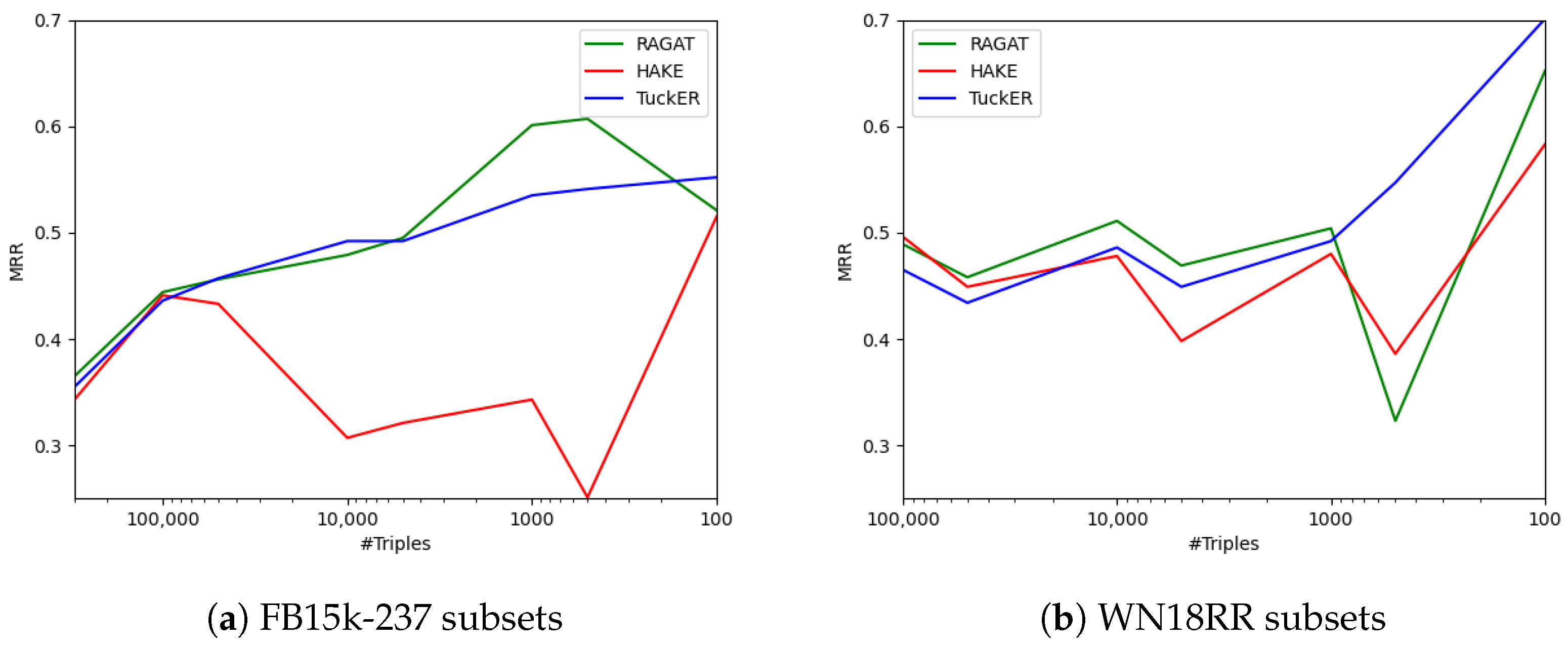
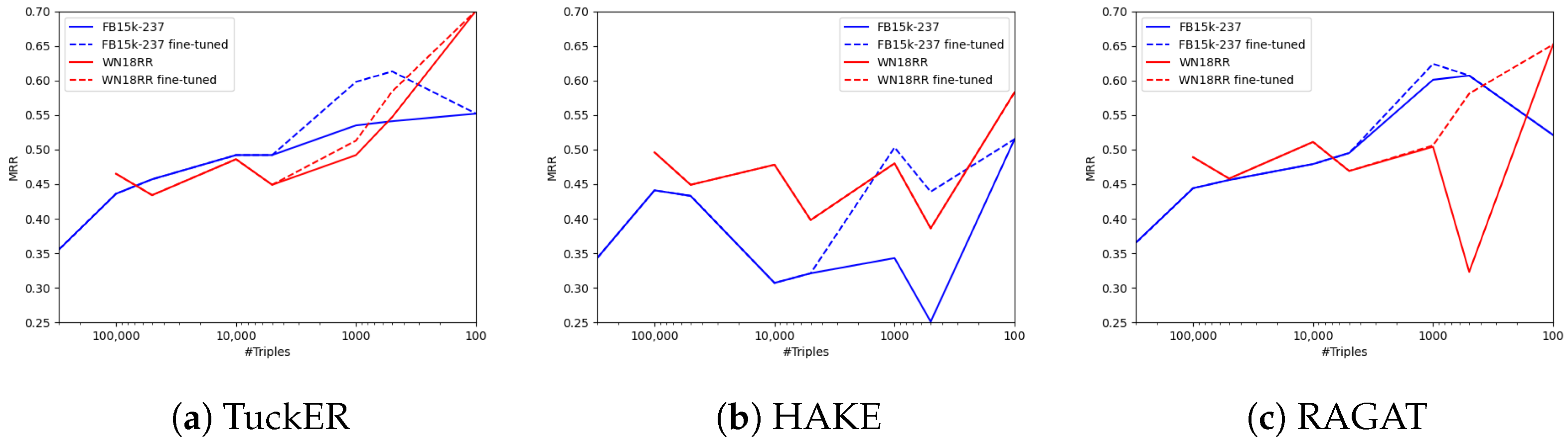
5.1. Performance Increase in Few-Shot Scenarios

The performance of TuckER as well as RAGAT increased on the FB15k-237 subsets as the dataset size decreased. On the one hand, this was a positive trend. On the other hand, some improvement in the metrics was due to the design of the scenario. Once the number of entities decreased and, thus, there were fewer triples, an overall improvement in performance could be expected due to the reduction in the size of the search space. Hence, the scores obtained on these reduced datasets should not be compared to the scores obtained from the literature. A Hits@10 score of 0.5 was not as meaningful as on the original datasets. To illustrate this fact, consider the maximum possible triples against which a true triple from the test set is evaluated, comparing FB15k-237 and FB100: In FB15k-237, there are a total of 14,541 entities. For a triple ( h , r , t ) , the head entity is replaced by each possible other entity in the evaluation, and the same is carried out for the tail entity to generate a set of triples against which the true triple is ranked. On FB15k-237, the maximum number of candidate triples is t = 14 , 541 for each of the sets. Compared to this, the maximum number of candidate triples on FB100 is t = 60 . In this case, due to the filtered settings, whereby all known true triples are also removed from the candidate set, there are in general fewer triples in both sets. Subsequently, it becomes statistically easier to rank true triples higher, as the number of possible entities decreases. Therefore, the models did not necessarily capture the information in the smaller subsets better than before, but it was easier to achieve better performance in terms of the metrics. However, the results still showed that the tested models were able to adapt to few-shot learning, thus achieving the evaluation goals.

5.2. RAGAT Performance Drop

The performance drop of RAGAT on WN500 was the most significant change in performance across all models. Since this only happened for this specific dataset, there must have been certain characteristics that influenced this change in performance. Following [51], relations can be categorized into four groups depending on the number of different heads and tails that they usually connect. The categories are assigned by calculating two scores for each relation: the tph (‘tails per head’), which indicates the average number of different tails that are connected to a head via the investigated relation, and the hpt (‘heads per tail’), which indicates the average number of different heads that are connected to a tail via the relation. Formalized, they can be defined as follows:
Definition 5.
For a fixed relation r, let H r be the set of entities that appear in a triple with relation r as the head entity, and T r the set of entities that appear as the tail entity. Furthermore, let T be the set of triples. Then, t p h can be defined as
t p h = 1 | H r | h r H r | { t : ( h r , r , t ) T } | ,
and h p t can be defined as
h p t = 1 | T r | t r T r | { h : ( h , r , t r ) T } | .
Relations are categorized as n − n relations if both tph and hpt are greater than 1.5, 1 − 1 if both are smaller than 1.5, n − 1 if tph < 1.5 and hpt 1.5 , and finally 1 − n if tph 1.5 and hpt < 1.5 , as summarized in Table 7.
The distribution of the different relation categories in the test set can be observed in Table 8. In the FB15k-237 subsets, the original distribution showed that the most frequent relation category was n − n, followed by n − 1. The 1 − n and 1 − 1 relations comprised a smaller part of the dataset.
WN500 contained the highest fraction of 1 − n relations of all WN18RR subsets and no n − 1 relations at all. Furthermore, this subset included the largest number of 1 − 1 relations of all subsets. FB500 was similar to WN500, since it contained the most 1 − n relations of its dataset group and no n − 1 relations. However, in contrast to WN500, RAGAT performed best on FB500. Still, RAGAT’s performance for 1 − n relations was likely the reason why it scored comparatively badly on WN500. When examining Table 8 again, one can observe that in WN500 there were on average four different heads per 1 − n relation, while in FB500, there were 1.7, which was close to the minimum of 1. Furthermore, FB500 did not contain any 1 − 1 relations but comprised 28% n − n relations, which meant that the performance almost solely relied on the 1 − n relations. Therefore, one can make the assumption that RAGAT’s performance was strongly influenced by its performance on the heads of the 1 − n relations, which were easier to predict in the case of FB500 than in the case of WN500. This phenomenon could be seen in the reported results as well. For RAGAT, the performance in predicting the head and tail of a true triple is reported separately, which is why an analysis of these factors is possible. The performance on the two subsets separated into heads and tails is presented in Table 9.
It is observable that the performance on both subsets was better for the prediction of the head than the tail. For FB500, this effect was very prominent, improving the overall performance greatly, although the model achieved an MRR of 0.28 when predicting the tail. This was due to the more uneven distribution of 1 − n relations in FB500 as compared to WN500. This also explained why RAGAT performed better on FB500 than on FB100, where the relation categories were more evenly distributed.

5.3. HAKE Performance Gap

In Section 4.2, an large gap in the overall performance of HAKE between the FB15k-237 and WN18RR subsets was observed. In the original publication [26], it was stated that HAKE performed much better on WN18RR than on FB15k-237, since WN18RR contains more relations resembling hierarchical properties. This likely influenced the performance of HAKE on the FB15k-237 subsets. Since the performance slightly improved on FB1k and spiked on FB100, it can be concluded that these subsets likely contained more relations that could better be modeled in a hierarchical structure. Overall, due to its stable performance, TuckER is suitable as a basis for a recommender system. It was shown that the performance of this approach was not affected by various complex dataset characteristics. Thus, it can be assumed that this model would perform stably with hyperparameters tuned to datasets of a comparable structure. Since overall, RAGAT performed similarly to TuckER, it is also usable in a recommender system, while the hyperparameters need more fine-tuning on more complex datasets. Compared to the other approaches, HAKE should not be selected as a basis for a recommender system, since it is dependent on the dataset structure and performed more poorly than the other approaches. Since the Hits@1, 3, and 5 results are the most relevant for use in a recommender system, it should be noted that most models had a Hits@1 value above 0.5 for the smaller data sets, while they never reached a value above 0.7 for Hits@5. In general, most Hits@5 scores were around 0.6, implying that when using these approaches for recommender systems, the correct triple would on average show up in the top five recommendations in 60% of cases. This score was favorable overall, especially considering the fact that the Hits@1 score can be expected to be approximately 0.5. Furthermore, these scores could potentially still be improved by adding a feedback loop to the model, allowing it to learn from the user’s feedback. To conclude, it can be expected that these approaches will be successful if used as recommender systems for semantic modeling.

5.4. Comparison with Previous Studies

Previous studies can be divided into studies comparing link prediction approaches on common datasets such as FB15k-237 and WN18RR, and studies evaluating them on few-shot datasets. Extensive comparisons of link prediction approaches on different datasets were presented by Rossi et al. [43] and Ferrari et al. [44]. However, these authors used datasets with large numbers of triples and therefore did not provide insight into the performance of the approaches on small datasets. In comparison, Sheng et al. [47] evaluated different approaches on few-shot datasets. Using these datasets, the authors evaluated few-shot approaches as well as regular approaches and compared the results. However, few-shot datasets provide a specific number of triples per relation, which is not the case in more realistic scenarios. Moreover, some few-shot approaches use information from a given background knowledge graph, which was also not provided in our scenario. The use of sampled subsets of increasing size allowed a more realistic evaluation of the performance of link prediction models on smaller datasets, such as semantic models, compared to these previous studies. In addition, it allowed an estimation of how different approaches are likely to perform as the available data sizes begin to increase.

5.5. Summary

In conclusion, all candidate models from the different link prediction categories performed considerably well on smaller datasets. No tested model showed a significant decline in the measured MRR and Hits@{1,3,5,10}. However, some minor characteristics could be identified during the evaluation.
Both the product-based candidate (TuckER) and the neural-network-based candidate (RAGAT) showed an improvement in performances for decreasing dataset sizes on both tested datasets. In addition, TuckER was found to be the most robust approach over all dataset sizes, as its performance was not influenced by different dataset characteristics. In comparison, RAGAT performed similarly but with slightly lower measurements.
HAKE, the candidate algorithm of the translational models, performed similarly to the other two models on the subsets of one dataset, but showed a decrease in performance on the other. The reason for this may have been related to HAKE’s internal structure, which favors hierarchical data structures, showing a dependency on certain dataset characteristics. It is therefore not generally applicable to few-shot scenarios. However, as this is only one selected model from the set of translational link prediction models, there may be a more suitable approach in this group.
In the subsequent hyperparameter optimization, performance improvements were observed for each candidate approach. The optimization particularly benefited HAKE and RAGAT, while TuckER’s performance showed only minor improvements, highlighting TuckER as a promising approach for managing link prediction in few-shot learning scenarios using a one-size-fits-all default configuration.

6. Conclusions and Outlook

In this paper, the performance of three link prediction models on small datasets (few-shot scenarios) was examined. Based on a comparative literature review, three representative approaches (TuckER [21], HAKE [16], and RAGAT [42]) were selected from different link prediction model categories: product-based, translational, and neural-network-based, respectively. Thirteen subsets of two common datasets used for link prediction (FB15k-237 and WN18RR) were created, on which the respective link prediction models were evaluated using their original hyperparameter settings. TuckER, the product-based model, showed steady improvements in its performance as the size of the subsets decreased. HAKE, the translation-based model, showed performances dependent on the characteristics of the datasets. RAGAT, the neural-network-based model, demonstrated a performance closer to that of TuckER, but it was likely influenced by the distribution of relations contained in the training data. During the experiments, most models achieved higher performance scores on the smaller subsets than on their original evaluation datasets. In addition, a grid search was performed on selected subsets for each of the approaches. These experiments showed that the shortcomings of RAGAT and HAKE with respect to certain datasets could be mitigated by applying the right set of hyperparameters. Still, even with fine-tuned hyperparameters, HAKE performed worse than RAGAT and TuckER. In conclusion, of the three studied link prediction methods, two achieved suitable results on smaller subsets.
For future work, we plan to evaluate novel approaches and include another dataset (i.e., Wikidata) for evaluation. Based on the current findings, the identified link prediction approaches will also be compared against existing few-shot algorithms, using few-shot datasets in the evaluation. In addition, both RAGAT and TuckER will be integrated into a semantic modeling framework (i.e., PLASMA [10]) to evaluate their suitability as part of a recommender system for semantic modeling when applied in a scenario with sparse training data.

Author Contributions

Conceptualization, R.B., A.P. (Alexander Paulus) and A.P. (André Pomp); methodology, R.B. and A.P. (Alexander Paulus); software, R.B.; validation, R.B. and A.P. (Alexander Paulus); formal analysis, R.B.; investigation, R.B. and A.P. (Alexander Paulus); data curation, R.B.; writing—original draft preparation, R.B. and A.P. (Alexander Paulus); writing—review and editing, R.B., A.P. (Alexander Paulus), A.P. (André Pomp) and T.M.; supervision, A.P. (Alexander Paulus), A.P. (André Pomp) and T.M.; project administration, A.P. (Alexander Paulus) and T.M. All authors have read and agreed to the published version of the manuscript.

Funding

This research received no external funding.

Data Availability Statement

The datasets used in this publication are available at https://github.com/TimDettmers/ConvE (accessed on 14 May 2023). Code used for the dataset subset sampling is available at https://github.com/Rebecca-Braken/Few-Shot-Sampling (accessed on 14 May 2023).

Conflicts of Interest

The authors declare no conflict of interest.

Appendix A. Grid Search Parameters, Space, and Results

Appendix A.1. TuckER

TuckER’s originally considered hyperparameters were the learning rate lr, the learning decay rate dr, the embedding dimension for the entities edim, the embedding dimension for the relations rdim, the input dropout in_d, two parameters for hidden dropout H_d1 and H_d2, a parameter for label smoothing ls, and the batch size batch. We followed the authors of the original study and used the specified hyperparameters for our grid search. For the learning rate, the parameters used for this approach on other datasets were selected. The resulting grid search space for the grid search on TuckER can be found in Table A1. Table A2 shows the hyperparameters that were used in the evaluation, including the original hyperparameter settings as well as the fine-tuned parameters for WN1k, WN500, FB1k, and FB500, which yielded the results for TuckER shown in Table 6.
Table A1. The search space used for the grid search on TuckER for the datasets FB1k, WN1k, FB500, and WN500.
lrdredimrdimin_dH_d1H_d2lsbatch
0.00050.9930300.20.20.3032
0.0010.9952002000.30.40.50.164
0.0031--0.60.60.6-128
0.01---0.80.80.8--
Table A2. The hyperparameter configurations of TuckER, consisting of the originally used hyperparameters on FB15k-237 and WN18RR as well as the fine-tuned hyperparameters for FB1k, WN1k, FB500, and WN500 that achieved the results for TuckER shown in Table 6.
Datasetlrdredimrdimin_dH_d1H_d2lsbatch
FB15k-2370.000512002000.30.40.50.1128
WN18RR0.0031200300.20.20.30.1128
FB1k0.010.995200300.80.60.30.132
FB5000.010.992002000.30.80.6064
WN1k0.0050.9952002000.30.60.3032
WN5000.010.992002000.60.60.3064

Appendix A.2. HAKE

The considered hyperparameters for HAKE were its training batch size batch, negative sampling size n, embedding dimension dim, model-specific parameters γ and α , learning rate l r , test batch size test_batch, modulus weight mod_w, and phase weight phase_w. The grid search space for HAKE can be found in Table A3. The training steps were chosen to be equivalent to the originally fine-tuned training steps for FB15k-237. For the modulus and phase weight, the constraint mod_w ≤ phase_w was added, as recommended by the authors [16]. In general, the search space was chosen according to the existing parameters as well as the information provided on GitHub (cf. https://github.com/MIRALab-USTC/KGE-HAKE/issues/3 (accessed on 14 May 2023)) and the parameters defined in RotatE. The best-performing hyperparameter combinations for HAKE on different datasets are visualized in Table A4.
Table A3. The search space used for the grid search on HAKE for the datasets FB1k, WN1k, FB500, and WN500.
batchndim γ α lrtest_batchmod_wphase_w
2565121000910.011644
12825650060.50.00183.52
64641253-0.00005-11
-------0.50.5
Table A4. The hyperparameter configurations of HAKE, consisting of the originally used hyperparameters on FB15k-237 and WN18RR as well as the fine-tuned hyperparameters for FB1k, WN1k, FB500, and WN500 that achieved the results for HAKE shown in Table 6.
Datasetbatchndim γ α lrtest_batchmod_wphase_w
FB15k-2375122561000910.00005163.51
WN18RR51251250060.50.0000580.50.5
FB1k256256500610.001814
FB500128256500610.011644
WN1k12864500310.0011611
WN500128256125610.011611

Appendix A.3. RAGAT

For RAGAT, the original hyperparameters were the number of epochs; composition operation; dropout in the graph convolutional network layer gcn_drop; batch size batch; number of attention heads H; and some InteractE-specific parameters including feature dropout ifeat_drop, dropout for the hidden layer ihid_drop, kernel size iker_sz, and number of permutations iperm. Since the composition operation from CrossE worked best in the original publication, it was chosen for the subsets as well. Furthermore, the number of epochs was fixed at 1500. The searched hyperparameter space is shown in Table A5. The InteractE hyperparameters were chosen according to the values recommended in the original publication [40]. For the batch size, smaller sizes compared to the original datasets were chosen to match the dataset sizes. The best performing hyperparameters are shown in Table A6.
Table A5. The search space used for the grid search on RAGAT for the datasets FB1k, WN1k, FB500, and WN500.
gcn_dropbatchifeat_dropihid_dropiker_szipermH
0.32560.20.3511
0.41280.40.5722
-640.6-94-
----11--
Table A6. The hyperparameter configurations of RAGAT, consisting of the originally used hyperparameters on FB15k-237 and WN18RR as well as the fine-tuned hyperparameters for FB1k, WN1k, FB500, and WN500 that achieved the results for RAGAT shown in Table 6.
Datasetgcn_dropbatchifeat_dropihid_dropiker_szipermH
FB15k-2370.42560.20.31111
WN18RR0.410240.40.3941
FB1k0.3640.60.51112
FB5000.3640.60.3942
WN1k0.3640.40.3512
WN5000.4640.20.51122

References

  1. Seagate; IDC. Rethink Data: Put More of Your Business Data to Work—From Edge to Cloud; Technical Report; Seagate Technology: Fremont, CA, USA, 2020. [Google Scholar]
  2. Halevy, A. Why Your Data Won’t Mix. Queue 2005, 3, 50–58. [Google Scholar] [CrossRef]
  3. Kamm, S.; Jazdi, N.; Weyrich, M. Knowledge Discovery in Heterogeneous and Unstructured Data of Industry 4.0 Systems: Challenges and Approaches. Procedia CIRP 2021, 104, 975–980. [Google Scholar] [CrossRef]
  4. Pomp, A.; Paulus, A.; Kirmse, A.; Kraus, V.; Meisen, T. Applying Semantics to Reduce the Time to Analytics within Complex Heterogeneous Infrastructures. Technologies 2018, 6, 86. [Google Scholar] [CrossRef]
  5. International Data Spaces Association. Reference Architecture Model: Version 3.0; International Data Spaces Association: Dortmund, Germany, 2019. [Google Scholar]
  6. GAIA-X European Association for Data and Cloud. Gaia-X Architecture Document. Available online: https://docs.gaia-x.eu/technical-committee/architecture-document/22.10/ (accessed on 14 May 2023).
  7. Paulus, A.; Pomp, A.; Poth, L.; Lipp, J.; Meisen, T. Recommending Semantic Concepts for Improving the Process of Semantic Modeling. In Proceedings of the Enterprise Information Systems—20th International Conference, ICEIS 2018, Funchal, Madeira, Portugal, 21–24 March 2018; Hammoudi, S., Smialek, M., Camp, O., Filipe, J., Eds.; Revised Selected PapersLecture Notes in Business Information Processing. Springer: Berlin, Germany, 2018; Volume 363, pp. 350–369. [Google Scholar] [CrossRef]
  8. Studer, R.; Benjamins, V.R.; Fensel, D. Knowledge Engineering: Principles and Methods. Data Knowl. Eng. 1998, 25, 161–197. [Google Scholar] [CrossRef]
  9. Futia, G.; Vetrò, A.; Martin, J.C.D. SeMi: A SEmantic Modeling machIne to build Knowledge Graphs with graph neural networks. SoftwareX 2020, 12, 100516. [Google Scholar] [CrossRef]
  10. Paulus, A.; Burgdorf, A.; Puleikis, L.; Langer, T.; Pomp, A.; Meisen, T. PLASMA: Platform for Auxiliary Semantic Modeling Approaches. In Proceedings of the 23rd International Conference on Enterprise Information Systems, ICEIS 2021, Online Streaming, 26–28 April 2021; Filipe, J., Smialek, M., Brodsky, A., Hammoudi, S., Eds.; SCITEPRESS: Setúbal, Portugal, 2021; Volume 2, pp. 403–412. [Google Scholar] [CrossRef]
  11. Paulus, A.; Burgdorf, A.; Stephan, A.; Pomp, A.; Meisen, T. Using Node Embeddings to Generate Recommendations for Semantic Model Creation. In Proceedings of the ICEIS 2022—24th International Conference on Enterprise Information Systems, Online, 25–27 April 2022. [Google Scholar] [CrossRef]
  12. Paulus, A.; Burgdorf, A.; Pomp, A.; Meisen, T. Collaborative Filtering Recommender System for Semantic Model Refinement. In Proceedings of the 2023 IEEE 17th International Conference on Semantic Computing (ICSC), Laguna Hills, CA, USA, 1–3 February 2023. [Google Scholar]
  13. Sun, Z.; Deng, Z.; Nie, J.; Tang, J. RotatE: Knowledge Graph Embedding by Relational Rotation in Complex Space. In Proceedings of the 7th International Conference on Learning Representations, ICLR 2019, New Orleans, LA, USA, 6–9 May 2019. [Google Scholar]
  14. Parnami, A.; Lee, M. Learning from Few Examples: A Summary of Approaches to Few-Shot Learning. arXiv 2022, arXiv:2203.04291. [Google Scholar] [CrossRef]
  15. Bordes, A.; Usunier, N.; García-Durán, A.; Weston, J.; Yakhnenko, O. Translating Embeddings for Modeling Multi-relational Data. In Proceedings of the Advances in Neural Information Processing Systems 26: 27th Annual Conference on Neural Information Processing Systems 2013, Lake Tahoe, NV, USA, 5–8 December 2013; Burges, C.J.C., Bottou, L., Ghahramani, Z., Weinberger, K.Q., Eds.; Curran Associates Inc.: Hook, NY, USA, 2013; pp. 2787–2795. [Google Scholar]
  16. Zhang, Z.; Cai, J.; Zhang, Y.; Wang, J. Learning Hierarchy-Aware Knowledge Graph Embeddings for Link Prediction. In Proceedings of the Thirty-Fourth AAAI Conference on Artificial Intelligence, New York, NY, USA, 7–12 February 2020. [Google Scholar] [CrossRef]
  17. Balazevic, I.; Allen, C.; Hospedales, T.M. Hypernetwork Knowledge Graph Embeddings. In Proceedings of the Artificial Neural Networks and Machine Learning–ICANN 2019: Workshop and Special Sessions: 28th International Conference on Artificial Neural Networks, Munich, Germany, 17–19 September 2019; Springer: Berlin, Germany, 2019; pp. 553–565. [Google Scholar]
  18. Nathani, D.; Chauhan, J.; Sharma, C.; Kaul, M. Learning Attention-based Embeddings for Relation Prediction in Knowledge Graphs. arXiv 2019, arXiv:1906.01195. [Google Scholar]
  19. Ali, M.; Berrendorf, M.; Hoyt, C.T.; Vermue, L.; Galkin, M.; Sharifzadeh, S.; Fischer, A.; Tresp, V.; Lehmann, J. Bringing Light Into the Dark: A Large-scale Evaluation of Knowledge Graph Embedding Models under a Unified Framework. IEEE Trans. Pattern Anal. Mach. Intell. 2021, 44, 8825–8845. [Google Scholar] [CrossRef]
  20. Nickel, M.; Tresp, V.; Kriegel, H. A Three-Way Model for Collective Learning on Multi-Relational Data. In Proceedings of the 28th International Conference on Machine Learning, ICML 2011, Bellevue, WA, USA, 28 June–2 July 2011; Getoor, L., Scheffer, T., Eds.; Omnipress: Madison, WI, USA, 2011; pp. 809–816. [Google Scholar]
  21. Balazevic, I.; Allen, C.; Hospedales, T.M. TuckER: Tensor Factorization for Knowledge Graph Completion. arXiv 2019, arXiv:1901.09590. [Google Scholar]
  22. Yang, B.; Yih, W.; He, X.; Gao, J.; Deng, L. Embedding Entities and Relations for Learning and Inference in Knowledge Bases. In Proceedings of the 3rd International Conference on Learning Representations, ICLR 2015, San Diego, CA, USA, 7–9 May 2015; Bengio, Y., LeCun, Y., Eds.; Conference Track Proceedings. [Google Scholar]
  23. Trouillon, T.; Welbl, J.; Riedel, S.; Gaussier, É.; Bouchard, G. Complex Embeddings for Simple Link Prediction. arXiv 2016, arXiv:1606.06357. [Google Scholar]
  24. Nickel, M.; Rosasco, L.; Poggio, T.A. Holographic Embeddings of Knowledge Graphs. In Proceedings of the Thirtieth AAAI Conference on Artificial Intelligence, Phoenix, AZ, USA, 12–17 February 2016; Schuurmans, D., Wellman, M.P., Eds.; AAAI Press: Washington, DC, USA, 2016; pp. 1955–1961. [Google Scholar]
  25. Hayashi, K.; Shimbo, M. On the Equivalence of Holographic and Complex Embeddings for Link Prediction. arXiv 2017, arXiv:1702.05563. [Google Scholar]
  26. Zhang, S.; Tay, Y.; Yao, L.; Liu, Q. Quaternion Knowledge Graph Embeddings. arXiv 2019, arXiv:1904.10281. [Google Scholar]
  27. Tucker, L.R. The Extension of Factor Analysis to Three-Dimensional Matrices; Holt, Rinehart and Winston: New York, NY, USA, 1964; pp. 110–127. [Google Scholar]
  28. Kazemi, S.M.; Poole, D. SimplE Embedding for Link Prediction in Knowledge Graphs. arXiv 2018, arXiv:1802.04868. [Google Scholar]
  29. Hitchcock, F.L. The expression of a tensor or a polyadic as a sum of products. J. Math. Phys. 1927, 6, 164–189. [Google Scholar] [CrossRef]
  30. Sun, Z.; Vashishth, S.; Sanyal, S.; Talukdar, P.P.; Yang, Y. A Re-evaluation of Knowledge Graph Completion Methods. arXiv 2019, arXiv:1911.03903. [Google Scholar]
  31. Wang, M.; Qiu, L.; Wang, X. A Survey on Knowledge Graph Embeddings for Link Prediction. Symmetry 2021, 13, 485. [Google Scholar] [CrossRef]
  32. Kipf, T.N.; Welling, M. Semi-Supervised Classification with Graph Convolutional Networks. arXiv 2016, arXiv:1609.02907. [Google Scholar]
  33. Gilmer, J.; Schoenholz, S.S.; Riley, P.F.; Vinyals, O.; Dahl, G.E. Neural Message Passing for Quantum Chemistry. In Proceedings of the 34th International Conference on Machine Learning, ICML 2017, Sydney, NSW, Australia, 6–11 August 2017; Precup, D., Teh, Y.W., Eds.; Proceedings of Machine Learning Research. PMLR: New York City, NY, USA, 2017; Volume 70, pp. 1263–1272. [Google Scholar]
  34. Schlichtkrull, M.; Kipf, T.N.; Bloem, P.; van den Berg, R.; Titov, I.; Welling, M. Modeling Relational Data with Graph Convolutional Networks. In Proceedings of the The Semantic Web: 15th International Conference, ESWC 2018, Heraklion, Crete, Greece, 3–7 June 2018; Proceedings 15. Springer: Berlin, Germany, 2018; pp. 593–607. [Google Scholar]
  35. Dettmers, T.; Minervini, P.; Stenetorp, P.; Riedel, S. Convolutional 2D Knowledge Graph Embeddings. arXiv 2017, arXiv:1707.01476. [Google Scholar] [CrossRef]
  36. Nguyen, D.Q.; Nguyen, T.D.; Nguyen, D.Q.; Phung, D.Q. A Novel Embedding Model for Knowledge Base Completion Based on Convolutional Neural Network. arXiv 2017, arXiv:1712.02121. [Google Scholar]
  37. Shang, C.; Tang, Y.; Huang, J.; Bi, J.; He, X.; Zhou, B. End-to-end Structure-Aware Convolutional Networks for Knowledge Base Completion. arXiv 2018, arXiv:1811.04441. [Google Scholar] [CrossRef]
  38. Ye, R.; Li, X.; Fang, Y.; Zang, H.; Wang, M. A Vectorized Relational Graph Convolutional Network for Multi-Relational Network Alignment. In Proceedings of the Twenty-Eighth International Joint Conference on Artificial Intelligence (IJCAI-19), Macao, China, 10–16 August 2019. [Google Scholar] [CrossRef]
  39. Vashishth, S.; Sanyal, S.; Nitin, V.; Talukdar, P.P. Composition-based Multi-Relational Graph Convolutional Networks. arXiv 2019, arXiv:1911.03082. [Google Scholar]
  40. Vashishth, S.; Sanyal, S.; Nitin, V.; Agrawal, N.; Talukdar, P. InteractE: Improving Convolution-based Knowledge Graph Embeddings by Increasing Feature Interactions. arXiv 2019, arXiv:1911.00219. [Google Scholar] [CrossRef]
  41. Veličković, P.; Cucurull, G.; Casanova, A.; Romero, A.; Liò, P.; Bengio, Y. Graph Attention Networks. arXiv 2017, arXiv:1710.10903. [Google Scholar]
  42. Liu, X.; Tan, H.; Chen, Q.; Lin, G. RAGAT: Relation Aware Graph Attention Network for Knowledge Graph Completion. IEEE Access 2021, 9, 20840–20849. [Google Scholar] [CrossRef]
  43. Rossi, A.; Barbosa, D.; Firmani, D.; Matinata, A.; Merialdo, P. Knowledge Graph Embedding for Link Prediction: A Comparative Analysis. arXiv 2021, arXiv:2002.00819. [Google Scholar] [CrossRef]
  44. Ferrari, I.; Frisoni, G.; Italiani, P.; Moro, G.; Sartori, C. Comprehensive Analysis of Knowledge Graph Embedding Techniques Benchmarked on Link Prediction. Electronics 2022, 11, 3866. [Google Scholar] [CrossRef]
  45. Xiong, W.; Yu, M.; Chang, S.; Guo, X.; Wang, W.Y. One-Shot Relational Learning for Knowledge Graphs. In Proceedings of the 2018 Conference on Empirical Methods in Natural Language Processing, Brussels, Belgium, 31 October–4 November 2018; Riloff, E., Chiang, D., Hockenmaier, J., Tsujii, J., Eds.; Association for Computational Linguistics: Cedarville, OH, USA, 2018; pp. 1980–1990. [Google Scholar] [CrossRef]
  46. Chen, M.; Zhang, W.; Zhang, W.; Chen, Q.; Chen, H. Meta Relational Learning for Few-Shot Link Prediction in Knowledge Graphs. In Proceedings of the 2019 Conference on Empirical Methods in Natural Language Processing and the 9th International Joint Conference on Natural Language Processing, EMNLP-IJCNLP 2019, Hong Kong, China, 3–7 November 2019; Inui, K., Jiang, J., Ng, V., Wan, X., Eds.; Association for Computational Linguistics: Cedarville, OH, USA, 2019; pp. 4216–4225. [Google Scholar] [CrossRef]
  47. Sheng, J.; Guo, S.; Chen, Z.; Yue, J.; Wang, L.; Liu, T.; Xu, H. Adaptive Attentional Network for Few-Shot Knowledge Graph Completion. In Proceedings of the 2020 Conference on Empirical Methods in Natural Language Processing, EMNLP 2020, Online, 16–20 November 2020; Webber, B., Cohn, T., He, Y., Liu, Y., Eds.; Association for Computational Linguistics: Cedarville, OH, USA, 2020; pp. 1681–1691. [Google Scholar] [CrossRef]
  48. Taheriyan, M.; Knoblock, C.A.; Szekely, P.; Ambite, J.L. Learning the semantics of structured data sources. J. Web Semant. 2016, 37–38, 152–169. [Google Scholar] [CrossRef]
  49. Toutanova, K.; Chen, D. Observed versus latent features for knowledge base and text inference. In Proceedings of the 3rd Workshop on Continuous Vector Space Models and their Compositionality, Beijing, China, 26–31 July 2015; Association for Computational Linguistics: Cedarville, OH, USA, 2015. [Google Scholar] [CrossRef]
  50. Ruffinelli, D.; Broscheit, S.; Gemulla, R. You CAN Teach an Old Dog New Tricks! On Training Knowledge Graph Embeddings. In Proceedings of the 8th International Conference on Learning Representations, ICLR 2020, Addis Ababa, Ethiopia, 26–30 April 2020. [Google Scholar]
  51. Wang, Z.; Zhang, J.; Feng, J.; Chen, Z. Knowledge Graph Embedding by Translating on Hyperplanes. In Proceedings of the Twenty-Eighth AAAI Conference on Artificial Intelligence, Québec City, QC, Canada, 27–31 July 2014; Brodley, C.E., Stone, P., Eds.; AAAI Press: Washington, DC, USA, 2014; pp. 1112–1119. [Google Scholar]
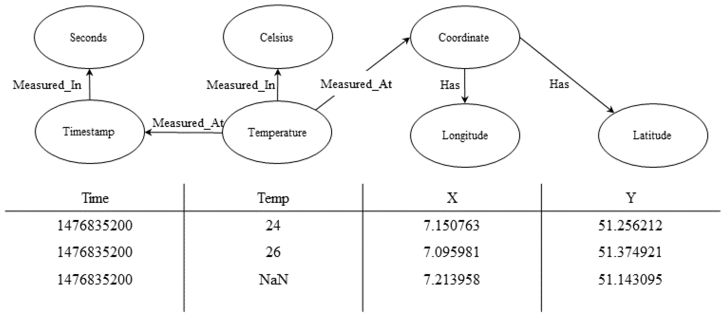
Figure 1. Example of a semantic model for Table 1.
Electronics 12 02296 g001
Figure 2. Example of the procedure chosen in the creation of a subset. The orange node represents the start node added to the subset. In the first step, this node was randomly sampled from the dataset. In later iterations, sampling was based on distance to the first node. The blue nodes represent edge nodes (of the subgraph), and the black nodes represent nodes that have already been processed.
Electronics 12 02296 g002
Figure 3. Overview of the performance of TuckER, HAKE, and RAGAT on the subsets of FB15k-237 and WN18RR. Dataset size is indicated on the x-axis, and the achieved MRR on the y-axis.
Electronics 12 02296 g003
Figure 4. Development of the models’ performances in terms of MRR for both dataset groups with and without optimized hyperparameters. The decreasing number of triples is presented on the (logarithmic) x-axis, and the MRR score is presented on the y-axis.
Electronics 12 02296 g004
Table 1. Example dataset.
TimeTempXY
1476835200247.15076351.256212
1476835200267.09598151.374921
1476835200NaN7.21395851.143095
Table 2. Dataset statistics of FB15K, WN18, and the reduced versions FB15K-237 and WN18RR.
Dataset# Entities# Relations# Triples
FB15k [15]14,9511345592,213
FB15k-237 [49]14,541237310,116
WN18 [15]40,94318151,442
WN18RR [35]40,9431193,003
Table 3. Evaluation results of different link prediction models on FB15k-237 and WN18RR. If a model was not evaluated on a specific dataset in the original publication, the source of the results is presented as well. The ‘Cat.’ column indicates the type of approach, where ‘P’ represents product-based, ‘T’ translational, and ‘N’ neural-network-based. The best results per dataset are in bold, and the second best results are underlined.
FB15k-237WN18RR
ModelCat.MRRHits@1Hits@3Hits@10MRRHits@1Hits@3Hits@10
RESCAL [20,50]P0.3560.2630.3930.5410.4670.4390.4800.517
TransE [15,50]T0.3130.2210.3470.4970.2280.0530.3680.520
DistMult [22,50]P0.3430.2500.3780.5310.4520.4130.4660.530
ComplEx [23,50]P0.3480.2530.3840.5360.4750.4380.4900.547
R-GCN [34]N0.1510.2640.417----
ConvE [35,50]N0.3390.2480.3690.5210.4420.4110.4510.504
ConvKB [18,36]N0.2890.1980.3240.4710.2650.0580.4450.558
SimplE [28,31]P0.1620.090.170.317----
HypER [17]N0.3410.2520.3760.5200.4650.4360.5160.582
SACN [37]N0.3500.260.390.540.470.430.480.54
RotatE [13]T0.3380.2410.3750.5330.4760.4280.4920.571
QuatE [26]P0.3480.2480.3820.5500.4880.4380.5080.582
TuckER [21]P0.3580.2660.3940.5440.470.4430.4820.526
CrossE [16]P0.2990.2110.3310.474----
VR-GCN [38]N0.2480.1590.2720.432----
CompGCN [39]N0.3550.2640.3900.5350.4790.4430.4940.546
Fixed KBGAT [30]N0.157--0.3310.412--0.554
HAKE [16]T0.3460.2500.3810.5420.4970.4520.5160.582
InteractE [40]N0.3540.263-0.5350.4630.43-0.528
RAGAT [42]N0.3650.2730.4010.5470.4890.4520.5030.562
Table 4. Dataset split sizes for the original FB15k-237 and WN18RR datasets as well as all subsets generated for the experiments.
IdentifierTriplesEntitiesRelations# Training# Validation# Test
FB15k-237310,11614,541237272,11517,53520,466
FB100k100,02811,45922685,02574497554
FB50k50,040982022342,52937053806
FB10k10,43557861698884743808
FB5k50192807914269359391
FB1k1016585318676980
FB500510399294383240
FB100109602695410
WN18RR93,0031140,94386,83530343134
WN50k50,00325,3861142,50337473753
WN10k10,0056131118505748752
WN5k50053347114252372379
WN1k100167278507576
WN50050834094323541
WN1001096369478
Table 5. Evaluation Results of the models on the different subsets defined in Section 3.1. The best results per subset are in bold.
DatasetModelMRRHits@1Hits@3Hits@5Hits@10
TuckER0.4360.3240.4950.5680.658
FB100kHAKE0.4410.3230.5110.5830.663
RAGAT0.4440.3330.5040.5750.658
TuckER0.470.4430.482-0.526
WN18RRHAKE0.4970.4520.516-0.582
RAGAT0.4890.4520.503-0.562
TuckER0.4570.360.5110.5720.639
FB50kHAKE0.4330.3320.4920.5550.617
RAGAT0.4560.360.5090.5710.639
TuckER0.4340.4180.4410.4510.466
WN50kHAKE0.4490.4190.4590.480.507
RAGAT0.4580.4290.470.4890.514
TuckER0.4920.4260.5270.5680.621
FB10kHAKE0.3070.250.3320.3760.416
RAGAT0.4790.4080.5150.5620.608
TuckER0.4860.4720.4940.4990.51
WN10kHAKE0.4780.4630.480.4890.508
RAGAT0.5110.4850.520.5370.557
TuckER0.4920.4250.5290.5660.623
FB5kHAKE0.3210.270.3440.3730.423
RAGAT0.4950.4230.5350.5820.637
TuckER0.4490.4180.4760.4910.5
WN5kHAKE0.3980.3760.3980.420.45
RAGAT0.4690.4290.4840.5170.544
TuckER0.5350.450.5880.6630.681
FB1kHAKE0.3430.2690.3880.4130.444
RAGAT0.6010.5380.6380.6690.706
TuckER0.4920.4670.4930.5130.533
WN1kHAKE0.480.4610.4930.50.507
RAGAT0.5040.4740.5070.5390.572
TuckER0.5410.4880.5750.6380.65
FB500HAKE0.2510.20.250.2750.3
RAGAT0.6070.550.6130.70.7
TuckER0.5470.5240.5490.5490.573
WN500HAKE0.3860.3780.3780.390.39
RAGAT0.3230.2440.3530.4090.465
TuckER0.5520.450.60.60.7
FB100HAKE0.5150.450.550.550.6
RAGAT0.5210.40.550.60.6
TuckER0.7010.6880.6880.6880.75
WN100HAKE0.5830.50.6250.6880.875
RAGAT0.6520.6250.6250.6250.813
Table 6. Performance of TuckER, HAKE, and RAGAT with the originally reported hyperparameter settings (‘Original’) and fine-tuned hyperparameters (‘Grid Search’). The best results per subset are in bold.
DatasetModelConfigurationMRRHits@1Hits@3Hits@5Hits@10
FB1kTuckEROriginal0.5350.450.5880.6230.681
TuckERGrid Search0.5980.5310.6310.6810.713
HAKEOriginal0.3430.2690.3880.4130.444
HAKEGrid Search0.5030.4310.550.5690.613
RAGATOriginal0.6010.5360.6380.6690.706
RAGATGrid Search0.6240.5690.6380.6750.7
TuckEROriginal0.5410.4880.5750.6380.65
TuckERGrid Search0.6130.5880.6250.650.65
FB500HAKEOriginal0.4390.3750.4750.4880.55
RAGATOriginal0.6070.550.6130.70.7
RAGATGrid Search0.6060.550.6130.650.688
TuckEROriginal0.4920.4670.4930.5130.533
TuckERGrid Search0.5130.4930.5130.5330.566
WN1kHAKEOriginal0.480.4610.4930.50.507
RAGATOriginal0.5040.4740.5070.5390.572
RAGATGrid Search0.5060.4740.5070.5390.572
TuckEROriginal0.5470.5240.5490.5490.573
TuckERGrid Search0.5840.5730.5850.5850.598
WN500HAKEOriginal0.3860.3780.3780.390.39
RAGATOriginal0.3230.2440.3530.4090.465
RAGATGrid Search0.5810.5490.5850.5850.646
Table 7. Categorization of relations depending on their hpt and tph scores.
Categoryhpttph
n − n≥1.5≥1.5
1 − 1<1.5<1.5
n − 1≥1.5<1.5
1 − n<1.5≥1.5
Table 8. Rounded percentage of each relation category in the test set.
Dataset# n − n# n − 1# 1 − n# 1 − 1
FB15k-23772%21%6%1%
FB100k72%17%10%1%
FB50k65%20%13%2%
FB10k26%47%24%2%
FB5k33%35%27%5%
FB1k39%39%20%3%
FB50028%0%73%0%
FB10050%20%30%0%
WN18RR36%47%15%1%
WN50k43%42%14%2%
WN10k47%44%7%2%
WN5k39%28%32%2%
WN1k50%45%0%5%
WN50037%0%41%22%
WN10062%38%0%0%
Table 9. Average number of different heads and tails for relation categories n − 1 and 1 − n.
DatasetCategoryMRRHits@1Hits@3Hits@5Hits@10
FB500Head0.9310.90.950.9750.975
Tail0.2830.20.2750.4250.425
Average0.6070.550.6130.70.7
WN500Head0.4520.3540.4750.5680.672
Tail0.1950.1350.2320.2510.258
Average0.3230.2440.3530.4090.465
Disclaimer/Publisher’s Note: The statements, opinions and data contained in all publications are solely those of the individual author(s) and contributor(s) and not of MDPI and/or the editor(s). MDPI and/or the editor(s) disclaim responsibility for any injury to people or property resulting from any ideas, methods, instructions or products referred to in the content.

