Abstract
Insulated overhead conductor (IOC) faults cannot be detected by the ordinary protection devices due to the existence of the insulation layer. The failure of insulated overhead conductors is regularly accompanied by partial discharge (PD); thus, IOC faults are often judged by the PDs of insulated overhead conductors. In this paper, an intelligent PD detection model based on bidirectional long short-term memory with attention mechanism (AM-Bi-LSTM) is proposed for judging IOC faults. First, the original signals are processed using discrete wavelet transform (DWT) for de-noising, and then the signal statistical-feature and entropy-feature vectors are fused to characterize the PD signals. Finally, an AM-Bi-LSTM network is proposed for PD detection, in which the AM is able to assign the inputs different weights and highlight their effective characteristics; thus, the identification accuracy and computational complexity have been greatly improved. The validity and accuracy of the proposed model were evaluated with an ENET common dataset. The experiment results demonstrate that the AM-Bi-LSTM model exhibits a higher performance than the existing models, such as LSTM, Bi-LSTM, and AM-LSTM.
1. Introduction
High-voltage overhead transmission lines, which are an important part of modern power systems, are increasingly using insulated overhead conductors. Compared with bare overhead conductors, insulated overhead conductors can prevent power outages caused by interline and line-to-ground failures, thereby improving the reliability of modern power systems. In addition, in terms of the environment, disturbances caused by forest fires, the electrocution of animals, and falling trees are mitigated by the use of insulating conductors [1,2]. However, ordinary protective devices, which are used for bare conductor systems, are unable to detect IOC faults without overcurrent. The IOC faults can cause partial discharge (PD) before breakdown [2,3,4,5]. Therefore, early partial discharge detection helps to ensure the high reliability and security of power grid assets. In other words, the emphasis of IOC fault detection has shifted from traditional current detection to PD detection. However, due to the small pulse value of the PD and interference from external background noise, fault detection through PD identification has become one of the most difficult challenges [3].
Due to the non-stationarity and randomness of PD signals, various types of time–frequency analysis methods, such as wavelet transform (WT), Hilbert–Huang transform (HHT), and S transform, have been proposed to analyze them. In [6], a simple algorithm, which works in four steps, including increasing the signal-to-noise ratio, removing DSI (discrete spectral interference) noise and RPI (random pulse interference) noise, and detecting PD, was created for automatic PD pattern detection. In [7], a fast approach is proposed for the detection of the partial discharge from the data collected by the antenna, and it had a small computational demand and low false-positive rate. In [8], two new features, namely, the template-matching degree and intracluster concentration degree, are proposed for the superior detection of PD based on light gradient-boosting machine (lightGBM).
While the above detection methods are effective, with the complexity of power systems increasing, fault diagnosis requires more efficient techniques to automatically extract multilevel features from large amounts of data. Therefore, fault detection methods based on deep learning have been widely applied to PD recognition. Reference [9] proposed a deep learning neural network model called the stacked sparse autoencoder (SSAE) to extract features from PD signals, and then the extracted features are fed into a softmax classifier to be classified into one of four defined PD severity states. In [10], the deep belief network is introduced for recognizing and classifying different PD patterns. In [11], to improve the recognition accuracy, a kind of PD pattern recognition method based on variational mode decomposition (VMD)–Choi–Williams distribution (CWD) spectrum and an optimized convolutional neural network (CNN) with cross-layer feature fusion is proposed. In [12], a new approach based on discrete wavelet transform (DWT) and a long short-term memory network (LSTM) is presented for the detection of IOC faults according to partial discharge. In [13], a multichannel CNN–LSTM (convolutional neural network, long short-term memory) network is proposed for fault detection by determining PD. In [14], a heterogeneous stacking ensemble neural network is applied to classify PDs obtained by the contactless method.
Although various deep learning models have been applied to the recognition of PD, the recognition accuracy and computation complexity still need to be further improved. First of all, all the models treat the input features equally and do not consider giving them different attention according to the correlation between each input feature and the recognition results. In addition, they are difficult to adapt to different background noises.
Recently, the attention mechanism (AM) [15,16] has emerged as a research hotspot in the field of deep learning. By assigning different weights to emphasize important information and ignore unimportant information, the AM offers higher accuracy, less computation time, and a better generalization ability. However, the existing work on PD recognition has not taken the AM into consideration.
To make better use of important information and ignore irrelevant information, this paper introduces the attention mechanism to the Bi-LSTM (bi-directional long short-term memory) framework. Furthermore, to reduce noise from the original PD signals, discrete wavelet transform (DWT) is proposed for denoising. Based on this, the Bi-LSTM model based on the AM and DWT is proposed for PD recognition. The key contributions of this paper are as follows: (1) a noise reduction technique based on DWT is proposed for denoising PD signals; (2) the AM is introduced for the PD recognition model, which can improve the recognition accuracy and computation complexity by emphasizing their effective characteristics; (3) Bi-LSTM, which combines past information and future information, has excellent time-series information-mining capability and makes PD recognition more accurate.
2. Proposed Fault Detection Method
In this section, PD detection based on Bi-LSTM with attention mechanism (AM-Bi-LSTM) in IOC faults is presented, which can automatically capture the most important features and achieve IOC fault detection. The proposed method depicted in Figure 1 mainly includes four steps: data pre-processing with DWT for denoising, feature extraction, the implementation of PD detection by AM-Bi-LSTM, and the evaluation of the detection results.
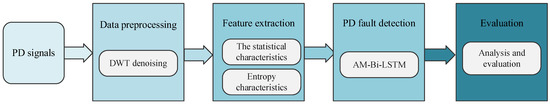
Figure 1.
Flow chart of the proposed PD detection method based on AM-Bi-LSTM.
2.1. Data Pre-Processing with DWT
PD measurement signals taken on-site are frequently affected by external disturbances (noise). To improve the detection accuracy, the PD signals need to be pre-processed for denoising. DWT is used for denoising in this paper.
A denoising method using wavelet theory takes wavelet coefficients by performing DWT on the measured PD signals and applies the appropriate threshold values for these coefficients. In other words, if the wavelet coefficient is smaller than the threshold value, then it may be caused by noise and carry only a small amount of signal information; otherwise, it may be caused by the original signal and carry a large amount of signal information. Thus, by ignoring these small wavelet coefficients and reconstructing the original signal using only the large wavelet coefficients, we can obtain a denoised version of the original PD signals.
In brief, the DWT-based denoising of PD signals includes three steps: signal decomposition, the thresholding of the coefficients, and reconstruction. In the first step, as shown in Figure 2, the noisy PD signal () is passed through a high-pass filter () and low-pass filter (), and then the detail coefficients and approximation coefficients can be obtained from the two filters at level one. The approximation coefficients are decomposed into two components by repeating the process at the next level. In this way, each level of the approximation signal is passed through orthogonal mirror filter pairs to obtain a higher proportion of approximation and detail coefficients.
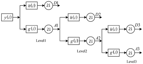
Figure 2.
Three-level multiresolution wavelet decomposition.
In the second step, the noise is removed by thresholding the detail coefficients at each decomposition level, generally using hard-thresholding and soft-thresholding methods. In the third step, after removing the noise in the detail coefficients and approximation coefficients, the denoising coefficients are used for the inverse decomposition process to obtain the enhanced PD signal, as shown in Figure 3. During the process of reconstruction, the approximation coefficients at the last level are added to the denoised detail coefficients of each level.
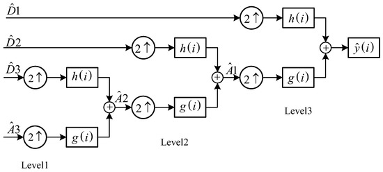
Figure 3.
Three-level multiresolution wavelet reconstruction.
2.2. The Proposed AM-Bi-LSTM
2.2.1. Bi-LSTM
The Bi-LSTM model [17] is built on a unidirectional LSTM network [18], which includes the forward LSTM network and reverse LSTM network. Both networks are connected to the same output layer, which completely captures past and future information in the input sequence. Figure 4 depicts the structure of the Bi-LSTM network. The hidden state () of the Bi-LSTM at time () includes the forward hidden state () and backward hidden state (), and they can be described as follows:
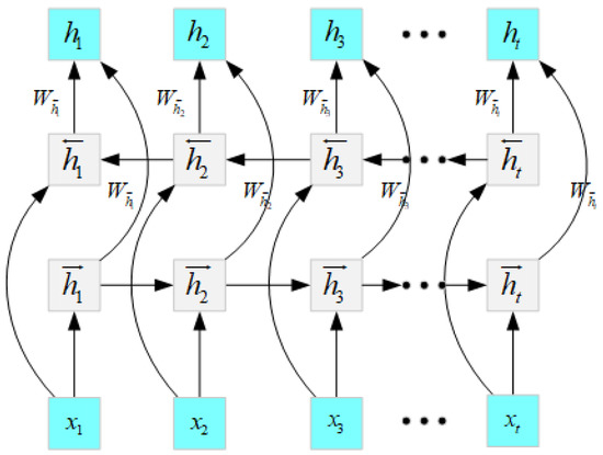
Figure 4.
The structure of the Bi-LSTM.
Here, is the input, and are the cell output state; and denote the weights of the , representing the biases; represents the activation function.
In Equation (1), both the hidden output states are updated by the standard LSTM theory. A single LSTM cell, shown in Figure 5, is made up of four components: a memory cell (), a forget gate (), an input gate (), and an output gate (), which can be depicted as follows:
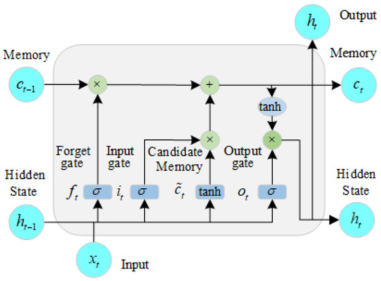
Figure 5.
The structure of the LSTM.
Here, , , , and denote the weight matrices of the forget gate, input gate, output gate, and memory cell, respectively; , , , and are the biases of the forget gate, input gate, output gate, and memory cell, respectively; denotes the temporary memory cell state; is the sigmoid activation function; denotes the tanh activation function; and × is the scalar product.
2.2.2. AM-Bi-LSTM
In order to facilitate the automatic concentration of the Bi-LSTM model on important information that has an important effect on detection, the attention mechanism is introduced to exploit the most decisive information. Figure 6 depicts the structure of the AM-Bi-LSTM.
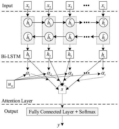
Figure 6.
The structure of the AM-Bi-LSTM.
In Figure 6, the attention mechanism can pay different attention to the different parts of the output () of the Bi-LSTM, which is defined as the weight of each part of the output (). The attention score can be defined as follows:
where , , and are the parameters in the attention gate. Then, the attention score () can be converted to the attention weight () by using a softmax function. is formulated as follows:
The attention weight () represents the contribution of each feature to PD detection. The weight hidden state () can be described as follows:
Then, the output (weight hidden state) is passed to a fully connected layer, which is used to determine PD faults.
The framework of the PD detection method based on Bi-LSTM with attention mechanism (AM-Bi-LSTM) in IOC faults can be described as in Figure 7.
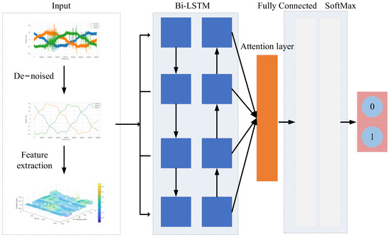
Figure 7.
The framework of the proposed detection method.
3. Simulation and Analysis
3.1. Data Analysis
The experimental dataset in this paper is from the ENET dataset (https://www.kaggle.com/competitions/vsb-power-line-fault-detection/data, accessed on 21 December 2018) published by the Technical University of Ostrava (VSB) in 2018, which devised a special instrument to measure PD signals. As shown in Figure 8, a single-layer coil is wrapped around the IOC to acquire the stray electrical field voltage along the IOC. Furthermore, a capacitive voltage divider is connected in parallel at the voltage output, and the output capacitor is connected in parallel with the inductor to obtain the voltage signal. VSB’s approach is more cost-effective than another possible solution that uses Rogowski sensors to directly measure currents in conductors [19].
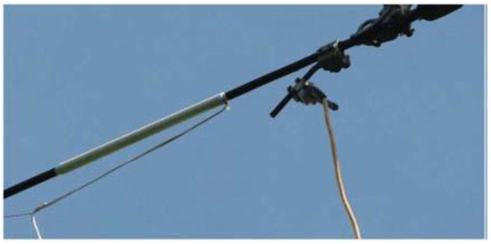
Figure 8.
The VSB’s PD measurement device for insulated overhead conductors in a medium-voltage system.
During the experimental measurement, the PD measurement device was placed at the end of the power system substation under the actual medium-voltage system and powered by a 5 km long IOC with a nominal phase voltage of 12.7 kV/50 Hz. The size of the IOC contact with the ground was gradually changed (e.g., spot contact: 1 m, 5 m, 10 m, and 35 m).
The ENET dataset includes signal data and metadata. The signal data contain 8712 voltage signals from four different locations, which represent the deployment in the real environment, such as forested and hard-to-access terrain. The metadata provide corresponding label information, namely, fault (1) or non-fault (0), and phase A (0), phase B (1), or phase C (2). Each voltage signal is a one-cycle voltage waveform with 800,000 sampling points at a sampling frequency of 40 MHz and was pre-marked as PD (525) or non-PD (8187). Figure 9 and Figure 10 show the signals without PD and with PD, respectively. Obviously, the two kinds of signals are disturbed by the external background noise, which reduces the accurate extraction of features. Compared with non-PD signals, PD signals have larger amplitudes (about 60 mV for PD and 40 mV for non-PD) and strong fluctuation. Data labels are shown in Table 1, which records the ID, phase, fault, and other important information of each data point.
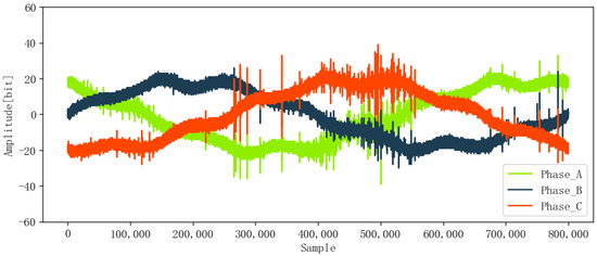
Figure 9.
Original signal without PD.
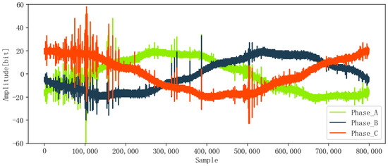
Figure 10.
Original signal with PD.

Table 1.
Data labels.
The signal_id is the number of each data point. Its index ranges from 0 to 8711, and there are 8712 data points in total. The Id_measurement represents the number of one group of three-phase signals. Phase depicts which phase the signal belongs to (0-A, 1-B, or 2-C), and target gives the fault result of the line, where 0 represents no fault (normal) and 1 represents fault.
3.2. PD Signal Denoising
When partial discharge occurs, each pulse signal contains unique information about the IOC’s specific state and fault features. The ENET dataset, acquired from real environments, such as forested and hard-to-access terrain, is subject to interference from external background noise. To improve the model’s anti-noise ability and ensure detection accuracy, it is crucial to reduce noise before feature extraction. In this paper, DWT was used for denoising the original signals, and Figure 11 and Figure 12 show the denoised signals, which are smoother than the original signals in Figure 9 and Figure 10.
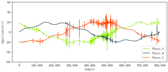
Figure 11.
Denoised signal without PD.
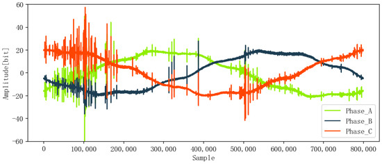
Figure 12.
Denoised signal with PD.
3.3. Feature Extraction
Feature extraction is the key to PD recognition. Although the voltage signal itself contains all the information, it is difficult to fit the original signal into some sets of rules and criterions that can intelligently interpret the potential information brought by the signal. In contrast, useful information is purposefully dug out by feature extraction. Additionally, reducing the dimensionality of the data can sometimes improve the performances of certain algorithms used in classifiers [20]. Thus, the statistical features and entropy features of PD signals were extracted in this study. Statistical features can reflect the morphological characteristics, while entropy features can characterize the time–frequency-spectrum complexity and detect small changes in PD signals. There are 19 statistical features, which include mean, std, mean plus std, mean minus std, seven percentiles, the amplitude, and seven relative percentiles. There are seven entropy features, which include perm entropy, singular entropy, approximate entropy, sample entropy, and three fractal dimensions. A one-phase PD signal has 19 statistical features; thus, three-phase PD signals have 57 dimensional features in all. The 57 dimensional features form a vector, which is depicted in Figure 13. Considering that the sample size was too large, a PD signal was divided into 160 subgroups, with 5000 data points in each subgroup. Hence, the statistical features extracted from all the subgroups were fused to form a 160 × 57 matrix, which is shown in Figure 14.
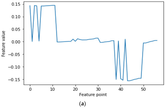
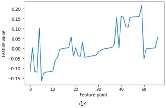
Figure 13.
The 57 dimensional statistical features of one subgroup. (a) Non-PD signal and (b) PD signal.
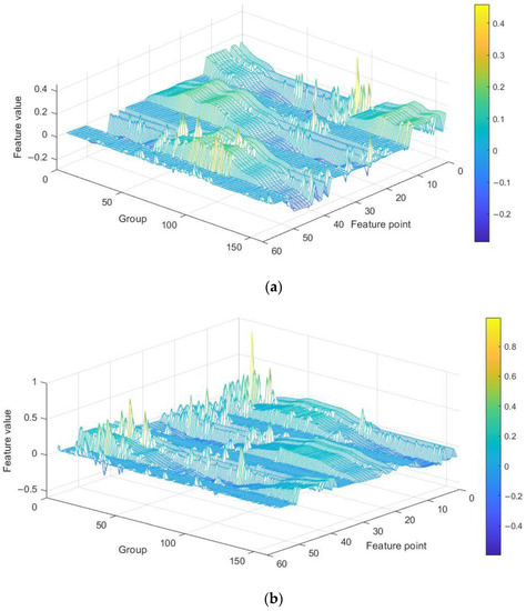
Figure 14.
Statistical features of one group PD signal. (a) Non-PD signal and (b) PD signal.
3.4. Model Evaluation
Python 3.6 was the development language used for the whole experiment in this paper, and the framework used to build the deep learning model was TensorFlow-GPU 1.13.2 and Keras 2.1.5.
This paper uses k-fold cross-validation to evaluate the model’s performance and prevent the improper selection of training and test sets from affecting the performance. Specifically, 5-fold cross-validation is used, as shown in Figure 15. The dataset is divided into five parts, with four used as training sets (green color represents training sets) and one as the test set (red color represents the test set). This process is repeated five times, and the average values are taken as the final result.
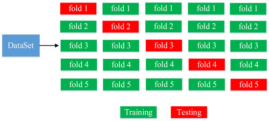
Figure 15.
Diagram for 5-fold cross-validation.
The parameter settings during the training are listed in Table 2. The optimization process is terminated when it reaches the maximum number of epochs. Figure 16 shows the loss values of one time during the training process and testing process. It can be seen that in about 40 generations, the training loss decreased slowly, the test loss almost did not change, and the values of them were reduced to about 0.07 in the end. Figure 17 displays the accuracy of the Matthew’s correlation coefficient at one time. It can be seen that when the training iteration reached about 20 times, the Matthew’s correlation coefficient fluctuated around 0.7, and the highest reached 0.78.
Table 2.
Parameter values.
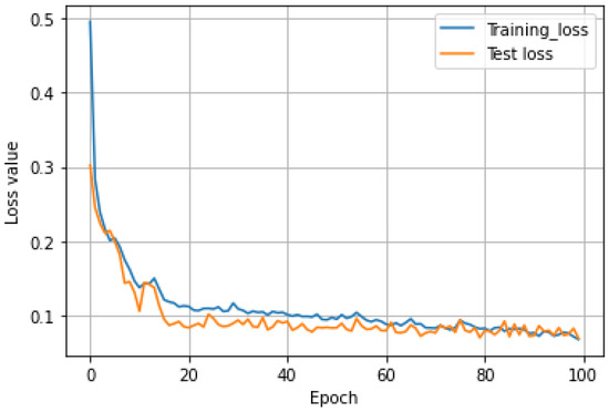
Figure 16.
The loss value of one time for training and testing.
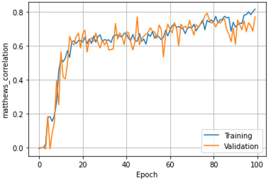
Figure 17.
The accuracy of one time for training and testing.
The confusion matrix is an intuitive representation of the model performance. Figure 18 shows the detection confusion matrix for the testing set one time. The rows represent the predicted results (including faults and non-faults), while the columns represent the actual results (including faults and non-faults). The diagonal elements correspond to correctly classified samples, while the off-diagonal elements correspond to misclassified samples. In other words, 537 non-fault samples and 25 fault samples are correctly classified, while 8 non-fault samples and 11 fault samples are misclassified.
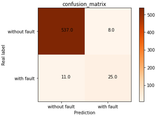
Figure 18.
The detection confusion matrix for testing set one time.
To thoroughly evaluate the proposed model’s effectiveness, several evaluation metrics were selected, including the accuracy rate, precision rate, recall rate, F1 score, and Matthew’s correlation coefficient (MCC) [21]. They are calculated as follows:
where TP is the correctly labelled positive signals, TN is the correctly labelled negative signals, FP is the incorrectly labelled positive signals, and FN is the incorrectly labelled negative signals.
Table 2 summarizes five corresponding evaluation indexes and their average values. It is evident from Table 3 that the training set and testing data have different accuracies, which reflects the necessity of K-fold cross-validation. Because there is a serious imbalance between failure samples and non-failure samples, non-failure samples have a better performance than failure ones in precision, recall, and F1. Accuracy is the most widely used evaluation index. The proposed method has an accuracy of about 97% for detecting faults and non-faults, indicating its effectiveness for PD detection. However, in the case of imbalanced fault and non-fault samples, the accuracy has a substantial defect. Therefore, it is far from scientific and comprehensive to evaluate a model only by its accuracy.
Table 3.
Cross-validation classification accuracy.
The recall rate reflects the ability of the model to identify positive samples, while the accuracy rate reflects the ability of the model to identify negative samples. The recall rate of non-fault samples is about 98.4%, and the recall rate of fault samples is about 75.9%, indicating that the model has a good ability to distinguish non-faults. The precision rate of non-fault samples is about 98.4%, and the precision rate of fault samples is about 77.1%, indicating that the model has a good ability to distinguish faults. F1 integrates the results of precision and recall, and the F1 of non-fault samples is about 98.4%, while that of fault samples is about 75.7%, indicating that the proposed method is effective for fault detection, and the model is very robust.
3.5. Algorithm Contrast
To demonstrate the superiority of the proposed AM-Bi-LSTM model, LSTM, Bi-LSTM, and attention-mechanism-based LSTM (AM-LSMT) were chosen for comparison to detect PD. During the comparison simulation, the parameter setting values of the other three models were the same as those of the proposed model. The detection results between different models are shown in Figure 19 and Figure 20. The performance of the AM-Bi-LSTM outperformed the other models in terms of the accuracy, F1, and MCC. Models with the attention mechanism, whether it is LSTM or Bi-LSTM, are better than the corresponding models without attention. This is because the model can pay different attention to the input features depending on their contribution to the detection results using the AM.
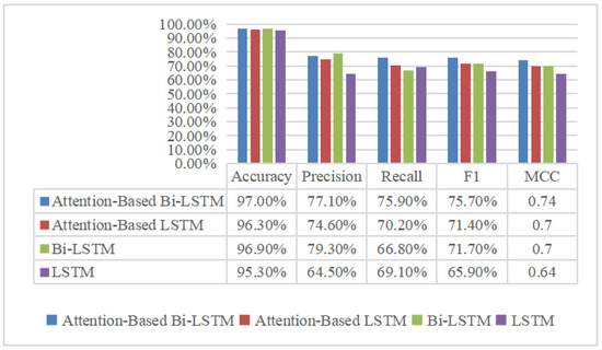
Figure 19.
Model performance comparison for PD detection.
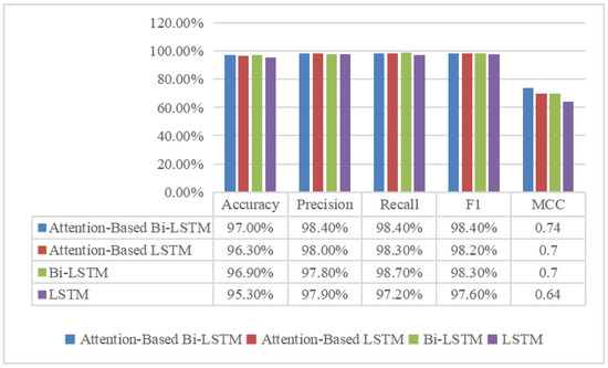
Figure 20.
Model performance comparison for non-PD detection.
In addition, in order to highlight the advantages of feature extraction in this paper, the evaluation index F1 is compared with the methods proposed in other papers, such as FNN (fuzzy neural network), SVM (support vector machine), XGBoost, and MLR in [12]. The comparison between these different methods is shown in Table 4. As can be seen from Table 4, the model proposed in this paper outperforms the other models in terms of effectiveness. In addition, due to the small proportion of fault data in the public dataset, the value of F1 obtained by the proposed model for fault samples is slightly higher than those obtained by other models, and the values of F1 for non-fault samples are far higher than those. It is worth mentioning that although these comparative algorithms in Table 4 are not the most advanced, they are the most widely used.
Table 4.
Comparison between different algorithms.
3.6. The Effect of Features on Results
Considering the importance of feature extraction, the PD classification results shown in Figure 21 are compared based on two different feature combinations. One is based on statistical features, and the other is based on the combination of statistical features and entropy features. Obviously, the accuracy, precision rate, recall rate, F1 score, and MCC based on the statistical features plus entropy features are superior to those based on only the statistical features. Specifically, the accuracy is increased by 0.4%, the precision rate is increased by 1.3%, the recall rate is increased by 6.8%, the F1 score is increased by 4.3%, and the MCC is increased by 0.4. However, it takes more time to extract entropy features than statistical features. Therefore, if high accuracy is required, statistical features plus entropy features can be selected, and if real time and efficiency are required, then only statistical features can be selected.
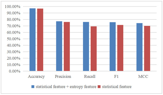
Figure 21.
Comparison of different features.
4. Conclusions
This paper proposes an AM-Bi-LSTM network to analyze and detect IOC faults based on PD signals. The model can combine past and future information for fault detection, and it can assign different weights to different information according to the correlation between each feature and the final detection by introducing the AM, which can improve the detection accuracy and computation complexity. The model’s effectiveness and accuracy were evaluated with the ENET public dataset, and the simulation results indicate that it outperformed the existing LSTM, Bi-LSTM, and AM-LSTM models. Moreover, the influences of different features on the classification results were compared, and the results show that the combination of statistical features and entropy features contributes to an improvement in accuracy.
Author Contributions
Conceptualization, Y.X.; Data curation, W.Z.; Writing—original draft, W.Z.; Writing—review & editing, F.Z. All authors have read and agreed to the published version of the manuscript.
Funding
This work was supported by the National Science Foundation of China (Grant No. 52277078), Natural Science Foundation of Hunan Province of China (Grant No. 2022JJ30609), and the Project of Education Bureau of Hunan Province, China (Grant No. 21A0210).
Data Availability Statement
All the data supporting the reported results have been included in this paper.
Conflicts of Interest
The authors declare no conflict of interest.
References
- Thomas, A.J.; Iyyappan, C.; Reddy, C.C. A method for surface voltage measurement of an overhead insulated conductor. IEEE Trans. Instrum. Meas. 2021, 70, 3021803. [Google Scholar] [CrossRef]
- Dong, M.; Sun, Z.X.; Wang, C. A pattern recognition method for partial discharge detection on insulated overhead conductors. IEEE Can. Conf. Electr. Comput. Eng. 2019, 2, 8861809. [Google Scholar]
- Soh, D.; Krishnan, S.B.; Abraham, J.; Xian, L.K.; Jet, T.K.; Yongyi, J.F. Partial discharge diagnostics: Data cleaning and feature extraction. Energies 2022, 15, 508. [Google Scholar] [CrossRef]
- Elaggoune, A.; Seghier, T.; Zegnini, B.; Mohammed, B. Partial discharge activity diagnosis in electrical cable terminations using neural networks. Trans. Electr. Electron. Mater. 2021, 22, 904–912. [Google Scholar] [CrossRef]
- Ma, D.; Jin, L.; He, J.; Gao, K. Classification of partial discharge severities of ceramic insulators based on texture analysis of UV pulses. High Volt. 2021, 6, 986–996. [Google Scholar] [CrossRef]
- Fulneček, J.; Mišák, S. A simple method for tree fall detection on medium voltage overhead lines with covered conductors. IEEE Trans. Power Deliv. 2021, 36, 1411–1417. [Google Scholar] [CrossRef]
- Martinovič, T.; Fulneček, J. Fast algorithm for contactless partial discharge detection on remote gateway device. IEEE Trans. Power Deliv. 2022, 37, 2122–2130. [Google Scholar] [CrossRef]
- Chen, K.J.; Vantuch, T.; Zhang, Y.; Hu, J.; He, J.L. Fault detection for covered conductors with high-frequency voltage signals: From local patterns to global features. IEEE Trans. Smart Grid 2021, 12, 1602–1614. [Google Scholar] [CrossRef]
- Tang, J.; Jin, M.; Zeng, F.P.; Zhang, X.X.; Huang, R. Assessment of PD severity in gas-insulated switchgear with an SSAE. IET Sci. Meas. Technol. 2017, 11, 423–430. [Google Scholar] [CrossRef]
- Karimi, M.; Majidi, M.; MirSaeedi, H.; Arefi, M.M.; Oskuoee, M. A novel application of deep belief networks in learning partial discharge patterns for classifying corona, surface, and internal discharges. IEEE Trans. Ind. Electron. 2020, 67, 3277–3287. [Google Scholar] [CrossRef]
- Gao, A.R.; Zhu, Y.L.; Cai, W.H.; Zhang, Y. Pattern recognition of partial discharge based on VMD-CWD spectrum and optimized CNN With cross-layer feature fusion. IEEE Access 2020, 8, 151296–151306. [Google Scholar] [CrossRef]
- Qu, N.; Li, Z.Z.; Zuo, J.K.; Chen, J.T. Fault detection on insulated overhead conductors based on DWT-LSTM and partial discharge. IEEE Access 2020, 8, 87060–87070. [Google Scholar] [CrossRef]
- Xi, Y.H.; Tang, X.; Li, Z.W.; Shen, Y.; Zeng, X.J. Fault detection and classification on insulated overhead conductors based on MCNN-LSTM. IET Renew. Power Gener. 2022, 16, 1425–1433. [Google Scholar] [CrossRef]
- Klein, L.; Seidl, D.; Fulneček, J.; Prokop, L.; Mišák, S.; Dvorský, J. Antenna contactless partial discharges detection in covered conductors using ensemble stacking neural networks. Expert Syst. Appl. 2023, 213, 118910. [Google Scholar] [CrossRef]
- Zhang, Z.; Zou, Y.; Gan, C. Textual sentiment analysis via three different attention convolutional neural networks and cross-modality consistent regression. Neurocomputing 2018, 275, 1407–1415. [Google Scholar] [CrossRef]
- Liu, G.; Guo, J. Bidirectional LSTM with attention mechanism and convolutional layer for text classification. Neurocomputing 2019, 337, 325–338. [Google Scholar] [CrossRef]
- Hochreiter, S.; Schmidhuber, J. Long short-term memory. Neural Comput. 1997, 9, 1735–1780. [Google Scholar] [CrossRef] [PubMed]
- Wang, S.X.; Wang, X.; Wang, S.M.; Wang, D. Bi-directional long short-term memory method based on attention mechanism and rolling update for short-term load forecasting. Electr. Power Energy Syst. 2019, 109, 470–479. [Google Scholar] [CrossRef]
- Mišák, S.; Pokorný, V. Testing of a covered conductor’s fault detectors. IEEE Trans. Power Deliv. 2015, 30, 1096–1103. [Google Scholar] [CrossRef]
- Chen, K.; Huang, C.; He, J. Fault detection, classification and location for transmission lines and distribution systems: A review on the methods. High Volt. 2016, 1, 25–33. [Google Scholar] [CrossRef]
- Chicco, D.; Jurman, G. The advantages of the Matthews correlation coefficient (MCC) over F1 score and accuracy in binary classification evaluation. BMC Genom. 2020, 21, 6. [Google Scholar] [CrossRef] [PubMed]


Disclaimer/Publisher’s Note: The statements, opinions and data contained in all publications are solely those of the individual author(s) and contributor(s) and not of MDPI and/or the editor(s). MDPI and/or the editor(s) disclaim responsibility for any injury to people or property resulting from any ideas, methods, instructions or products referred to in the content. |
© 2023 by the authors. Licensee MDPI, Basel, Switzerland. This article is an open access article distributed under the terms and conditions of the Creative Commons Attribution (CC BY) license (https://creativecommons.org/licenses/by/4.0/).