Abstract
Correctly anticipating PV electricity production may lessen stochastic fluctuations and incentivize energy consumption. To address the intermittent and unpredictable nature of photovoltaic power generation, this article presents an ensemble learning model (MVMD-CLES) based on the whale optimization algorithm (WOA), variational mode decomposition (VMD), convolutional neural network (CNN), long and short-term memory (LSTM), and extreme learning machine (ELM) stacking. Given the variances in the spatiotemporal distribution of photovoltaic data and meteorological features, a multi-branch character extraction iterative mixture learning model is proposed: we apply the MWOA algorithm to find the optimal decomposition times and VMD penalty factor, and then divide the PV power sequences into sub-modes with different frequencies using a two-layer algorithmic structure to reconstruct the obtained power components. The primary learner is CNN–BiLSTM, which is utilized to understand the temporal and spatial correlation of PV power from information about the weather and the output of photovoltaic cells, and the LSTM learns the periodicity and proximity correlation of the power data and obtains the corresponding component predictions. The second level is the secondary learner—the output of the first layer is learned again using the ELM to attenuate noise and achieve short-term prediction. In different case studies, regardless of weather changes, the proposed method is provided with the best group of consistency and constancy, with an average RMSE improvement of 12.08–39.14% over a single-step forecast compared to other models, the average forecast RMSE increased by 5.71–9.47% for the first two steps.
1. Introduction
In the context of maximum net-zero emissions and net-zero emissions, every country has agreed to aggressively contribute to the advancement of clean energy. Among these, photovoltaic energy production, as an important sustainable energy source in rapid development, plays a critical role in the safe, stable, and economical operation of electrical systems. However, the production of photovoltaic energy is sensitive to seasonal variations, meteorological conditions, diurnal variations, and the intensity of solar radiation, among other things, and presents a significant random and volatile character. Access to the large-scale photovoltaic grid poses a major challenge to the operational stability of the electricity system [1,2,3]. Therefore, the nicety prediction of photovoltaic electric energy production capacity is instrumental in formulating power generation plans, power dispatching, and promoting new energy consumption, effectively reducing operating costs and improving operational stability.
Physical models, statistical analysis models, artificial intelligence models, and hybrid models have been the focus of recent work on forecasting photovoltaic production [4]. Physical models compute photovoltaic power mainly from geographic and meteorological data and take into account environmental conditions such as solar radiation, humidity, and temperature as inputs to the model. Modeling is complex because the geographic and meteorological data for photovoltaic power stations need to be detailed to the best of their ability to anticipate the photovoltaic production. Statistical models often depict the link between historical time series. They generally include models of autoregressive rolling averages, quantum regression models, and integrated autoregressive rolling averages models, which gifted the merit of uncomplicated construction methods and the operating speed quickly. However, the models are suitable for stable series, while the actual PV data are highly variable with large errors [5]. The widely used intelligent metering device assembles an oversized quantity of real-world knowledge. Smart-meter integration and data facilitation provide novel possibilities for machine learning and in-depth learning to enhance the data-driven algorithm of photovoltaic power generation predictions.
1.1. Machine Learning
Several basic machine learning methods have been suggested in the literature [6,7] for predicting PV power, but none of them can accurately conduct multiple case studies. Transformations of data sets and transformations of internal parameters of machine learning models may yield different predictive results; these models suffer from volatility problems, where small data changes result in large changes in expected values, with poor stability and reliability.
Three machine learning techniques built using the RF, GTB, and SVM construction methodologies are presented in the literature [8]. The first two techniques, random forest and gradient augmentation, are integrated algorithms that combine multiple weak learners, and the results demonstrate that this combination results in more eclectic learning from the data [9]. Gradient boosting-based models are also found to ensure robust behavior and low prediction errors, as well as being more stable and able to lessen the uncertainty associated with the input data [10].
David Markovics et al. [11] stressed the need for a predictor selection and hyperparameter tuning to maximize model performance, especially for less robust models that tend toward under- or over-fitting without adequate tuning but still exhibit higher predictive performance for machine learning approaches when compared to baseline scenarios using linear regression. Since PV has a large variability on partially cloudy days and a low variability on bright days, other factors must be taken into account, such as short-term local weather patterns that may affect the area. Andrade et al. [12] created a prediction system by integrating XGBoost and a variety of feature engineering strategies to address this problem. The authors came to the conclusion that deep learning techniques outperform machine learning when properly combined with feature management.
1.2. Deep Learning
Deep learning (DL) is a renowned subfield of machine learning that has gained popularity in recent years and is frequently active across a variety of engineering specializations. As portrayed in learning features and the modeling of complicated interactions, deep learning models provide excellent prediction powers [13]. The most notable DLs-based PVPF models employed include the ELM [14,15], SVM [16], BP [17], CNN [18], and LSTM [19]—a numerous combination of structures. These approaches exhibited adaptability and accuracy in solar energy production predictions. With the continuous development of intelligent optimization algorithms, many scholars are committed to combining algorithms with deep learning networks, striving to find the optimal parameters of the model through optimization algorithms, such as using the PSO [20] to optimize Bi-LSTM, the SSA [21] to optimize LSTM models, and using the WOA [22,23] to optimize BiLSTM, ELM, etc. to reduce the impact of model parameters on prediction results and improve prediction accuracy.
The CNN can extract spatially correlated properties, enabling the study and investigation of non-linear correlations between time series data input and output. Convolutional neural networks were initially designed for image processing, and using 1DCNN for PV output time series data dramatically lowers locality invariance and cyclical portions when compared to 2DCNN, which is often used for image identification and extraction [18].
The LSTM model has shown the most promise in the PVPF and has been compared to other memoryless algorithms, such as the BP, MLR, and BRT. The literature [24] presents a PVPF system employing a CNN–LSTM network in combination with diverse meteorological factors, which performed better in terms of reliability and accuracy than conventional machine learning and individual DL models. The BiLSTM was initially proposed in 1997 and has been examined by simulation, and has excellent analytical accuracy and computing speed [25].
1.3. Data Decomposition
Hybrid models employ two or more approaches to extract the most value from available data from the past. Hybrid models primarily focus on integrating data deconstruction techniques with predictive models. The EMD, EEMD [26], and WT are frequently applied for irradiance forecasting; however, a wavelet packet transform must be artificially set to perform its fundamental function, which results in an inadequate flexibility and excessive reliance on individual subjectivity for prediction. Empirical modal decay is more adaptive but has the characteristics of the modal mixture.
Gao et al. [27] demonstrated that while the CEEMDAN–CNN–LSTM model beats benchmark models in diverse climates, the CEEMDAN–LSTM, CEEMDAN–BPNN, and CEEMDAN-SVM may better maintain spatial and temporal characteristics. The VMD is a Fourier transform-based non-recursive decomposition approach. In reference [28], the author proved the efficiency of the VMD, in which it outperformed the EMD and WT. Convolutional neural networks, which can filter and scale data, may be added to the suggested training framework to increase the prediction accuracy.
1.4. Predictive Models Based on Ensemble Learning
This integration method is often used in ensemble learning, where stacking can combine the predictions of different models in order to produce more accurate predictions than either model on its own. The authors in reference [29] offered a stacked model using XGboost, RF, and MLR as the preliminary layers of the stacked model and utilized their outputs to the linear Lasso model to assure an improved performance. The results of the comparison revealed that the connected models work more efficiently than the individual components selected for the comparisons. The integrated approach demonstrated that they are more stable and can reduce the uncertainty associated with entry data. The authors in reference [30] assessed the suggested model’s performance by comparing forecast outcomes with single ANN, LSTM, and Bagging. Despite weather fluctuations, the recommended DSE–XGB technique demonstrated the highest consistency and stability across case studies, and the whole model was far more precise and consistent than individual modeling.
1.5. Shortcomings of Existing Studies
The majority of earlier deep learning studies primarily looked at solar PV as a regression task, utilizing only basic statistical and artificial neural network models. It is difficult to anticipate solar PV time series data using solely computational intelligence techniques like artificial neural networks because of their dynamic behavior, autoregressive nature, and weather dependence. These techniques have a poor prediction ability because they cannot successfully characterize the behavior of nonlinear time series.
A hybrid prediction model called the PCC–EEMD–SSA–LSTM is suggested in the literature [31]. It used multidimensional data for one-step ahead prediction from prediction inputs using Pearson correlation coefficients to select more strongly correlated feature inputs, data decomposition, reconstruction evaluation using sample entropy, and the Sparrow algorithm to optimize the LSTM parameters pertaining to a multi-link optimization. However, the number of IMFs for the decomposition is entirely determined empirically, which has an impact on the accuracy of the EEMD decomposition reconstruction of the signal. The prediction model’s operational expense is reduced by reconstructing them into high-, medium-, and low-frequency series based on SE values, but the forecast accuracy is also decreased. The literature [32] proposed a VMD–DAIWPSO–PSR–KELM prediction model. Singular spectrum analysis filtered the PV series, using the VMD and phase space reconstruction (PSR) to analyze historical power knowledge, and the PSO to retrieve the prime PSR and KELM parameters and predict future PV power. However, using the central frequency domain to compute the value of decomposition, the IMF ignored the effect of penalty factors on the decomposition results and only a single historical power factor was considered, and other relevant factors, such as meteorology, that affect the magnitude of PV power were not analyzed.
1.6. Innovative Aspects of the Study
There have been several studies on predicting PV power, as shown in Table 1. To address the limitations of previous research and produce more precise forecasts, this study combined data decomposition with deep learning networks, the CNN and LSTM models, using the ability of the LSTM to retain past information and the CNN to extract meteorological features from meteorological knowledge to provide outputs that aggregate the forecasts of each model using integrated modeling. The advantages of implementing the ELM as a meta-learner can be seen in quantifying the miscalculation of individual models and the uncertainty of data noise, which can overcome the limitations of conventional gradient-based networks—including slow speed and multiple input parameters—and therefore, improve the accuracy of predictions. The main contributions of this study include:

Table 1.
An overview of some recent solar forecasting models.
- A benchmark framework for forecasting the PV power over various forecast periods, in which an integrated model with deep superposition was developed. The optimized whale algorithm (MWOA) was used for the parameter search optimization of the variable modal decomposition, and a comparison of the search optimization results of different optimization algorithms—PSO, SSA, and WOA—was provided. The effects of penalty factors on decomposition results have rarely been explored in previous studies while using the central frequency domain to determine the number of decompositions that need to be reset. In this study, the decomposition using the MWOA—VMD data does not require hyper parametric optimization, converges quickly, and has a lower chance of hitting a local optimum.
- In order to provide a thorough comparison of individual deep learning models, hybrid models, and models taking into account the different prediction inputs, the CNN–BiLSTM models were used in this study to investigate, in detail, the various features associated with meteorological and PV variables, and the ability of the LSTM to retain past information was used to solve the problem.
- Using data from operational PV systems, the proposed model affirmed more accuracy at making predictions than either a single deep learning model or a more traditional approach.
In the remaining sections of the paper, the following structure was used: this paper’s methodology is laid out in Section 2. Section 3 provides the structure and specific implementation ideas of the model proposed in this article. Section 4 compares the proposed prediction system, the MVMD–CLES, with commonly used prediction models; and finally, Section 5 is the conclusion section.
2. Methodology
2.1. Optimizing VMD Principles Based on WOA
The PV power sequence is an unpredictable, irregular signal. The sequence can be divided into several sub-series for independent predictions to lessen the complexity and increase the prediction accuracy. Among the existing signal decomposition techniques, EMD is one of the commonly used signal decomposition methods, but the split eigenmode decomposition covers a wide band and is prone to modal confusion. eEMD, CEEMD, CEEMDAN, etc. alleviate the problem of modal confusion by adding white noise, but the decomposition time increases greatly after adding white noise. VMD can make up for these two shortcomings—so, this paper uses the VMD to decompose the power data. It divides the original information into component, VMD minimizes the sum of the estimated bandwidths of each component. To solve the optimization problem, penalty factors and Lagrange multipliers are introduced to transform the constrained variational problem into an unconstrained variational problem [35]. Equation (1) gives the unconstrained variation model.
The updated Equation (2) for each IMF frequency domain is generated mostly by utilizing the alternating direction multiplier technique. According to Equation (1), the final convergence yields modal components with the center frequency . Updated are the parameters and through Equations (3) and (4).
where indicates the noise tolerance; when the signal contains a strong noise, can be set to achieve a better denoising effect.
For a given parameter , if Equation (5) holds, then stop updating; otherwise, proceed with the iteration and outcome of the last and .
The WOA is a three-stage optimization method inspired by the humpback whale’s strategy for finding food [36,37].
2.1.1. Surrounding the Prey
Equation (6) describes how the WOA algorithm finds the ideal position by looking for agents to surround the target.
where is the number of current iterations; denotes the current optimal position; and is the current position. and are shown in the following Equation (7).
where is the maximum number of iterations, decays linearly with the increase of iterations; takes random values and keeps updating the position by adjusting the values of and .
2.1.2. Bubble Net Predation
The spiral updated position is by Equation (9).
where is the distance to the prey at the -th iteration; is a random value that falls between [−1, 1]; and is a constant factor defining the shape of the logarithmic spiral.
2.1.3. Search for Prey
To do a worldwide search, use to modify the search agent’s position, in accordance with Equation (10).
where is a random position vector.
The parameters and have an impact on how the VMD algorithm decomposes the original data. The empirical setting is likely to lead to an excessive decomposition loss and affect forecast results. As a result, it is worthwhile to find the ideal value of . This study proposes the entropy as the fitness function of the WOA algorithm in literature [38].
The entropy value of a time series signal might indicate its unpredictability. The more complicated and unpredictable a sequence is, the higher the entropy value of each IMF component created by the decomposition. The entropy number accurately represents the time series’ complexity and potential to develop new patterns. Expressing all the resulting individual IMF sequences as a probability distribution , we can calculate the information entropy—the formula is shown in (11). The value of the fitness function is obtained according to Equation (12).
To pick the ideal parameter combination, the two-parameter choices are also taken into account. The flow chart of the WOA–VMD optimization is shown in Figure 1.
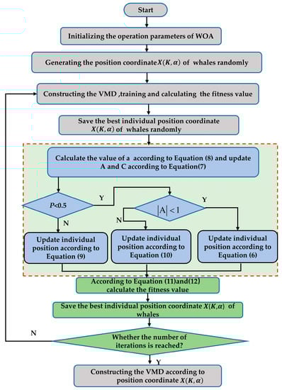
Figure 1.
The flow chart of the WOA–VMD optimization.
2.2. CNN–BiLSTM Network
The CNN, a popular deep neural network, has convolution, pool, and fully connected layers. In a multivariate time series prediction, it dynamically detects the high-level characteristics representation of a time series to collect significant information and performs a local connection and global sharing for many time series by a convolution operation. The CNN can accurately analyze correlations between variables. 1D-CNN layers usually simplify and enhance prediction models [24].
In this study, we used a stacked BiLSTM network as a key component of the model proposed, which offers the benefit of simultaneously capturing rich temporal information from various sequences [39]. The information from the appropriate time series’ history and future can be crucial in making predictions about the PV’s power. As a result, we maximize the bi-directional information in the PV correlation dataset by using the BiLSTM to figure out the relationship between the present and the previous and future time steps. The BiLSTM is an enhancement of the LSTM, an RNN variation that can solve the gradient vanishing issue by incorporating a pass selection algorithm. The whole is shown in the process in Equation (13). More contextual information is obtained in the historical observation of the entire input; the BiLSTM integrates the historical weather information in both directions and operates as shown in Equation (14).
where shows the input variable at the moment of , denotes the implicit layer state at the previous moment; reflects the unit memory state in the preceding instant; is the temporary memory state at moment ; and controls the quantity of data produced by the forgetting gate, updating gate, and memory unit, accordingly. represents the weights and biases used in the training procedure.
where indicates the hidden status of the forward layer at the moment of ; is the hidden state in the layer of backward at the time of ; and is the hidden state in the BiLSTM for the time of .
2.3. ELM Network
The ELM is a single-hidden layer supervised learning method. The ELM excels at modeling nonlinear information behavior in complex systems. The ELM outperforms the single-hidden layer feedforward neural network:
(1) Since the mapping functions of the hidden layers are known, once the optimal weights are chosen and then the output weights are determined analytically, the ELM model exhibits a significant estimation accuracy, which makes the ELM a fast learner. (2) It has a simple implementation, there is no need to artificially set a large number of training parameters before training. (3) It has a good generalization, whereby the challenge of generating local optimum solutions is not easily generated.
To estimate the PV plant’s power production, it is assumed that the training sample and the input variable is ,the expected output . The mathematical expression of the ELM model is
where are the input layer bias and the output layer bias, respectively; is the hidden layer bias; and is the activation function.
where is the desired output vector; and is the output of the implicit layer matrix, which can be expressed as
Apply the following Equation (18) to solve for the output weights.
where, is a generalized version of Moore’s inverse, which is applied to the matrix (Moore–Penrose).
2.4. Ensemble Stacked Model
Stacking usually uses heterogeneous integration and needs to satisfy the variability in the selection of base learners. In addition, since no single algorithm in the supervised learning domain can satisfy all the requirements of the task, Stacking also needs to focus on matching the task requirements and data characteristics to strive for all-around performance. The pseudocode of the stacking algorithm is as follows—Algorithm 1.
| Algorithm 1: Stacking algorithm. |
| Input: Training set: |
| Elementary learning algorithms: |
| Secondary learning algorithm: ; |
Procedures 1–3 include elementary learners who have had formal instruction. Processes 5–9 use anticipated results of training individual learners as the training set for the secondary learners. Process 11 is to train the secondary learners using the initial learners’ forecast outputs to create our final trained model.
3. Power Prediction Model for Photovoltaic Based on MVMD-CLES
The MVMD–CLES is based on the whale optimization algorithm (WOA), variational mode decomposition (VMD), convolutional neural network (CNN), long and short-term memory (LSTM), and extreme learning machine (ELM) stacking. The summary of the entire procedure is presented in Figure 2. The specific implementation steps of the proposed photovoltaic power generation prediction model were as follows:
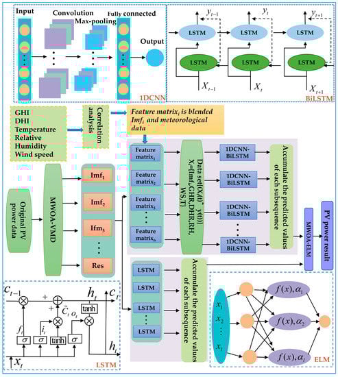
Figure 2.
Diagram of the predictive system MVMD–CLES structure.
Step 1: Carry out the outlier detection and data normalization for the PV historical data, and divide it into training samples, validation samples, and testing samples;
Step 2: Using the optimal parameter combination of the trained VMD decomposition, the collected photovoltaic power data is subjected to the VMD modal decomposition using a constrained variational model to obtain several historical power components of the VMD decomposition. The optimal parameter combination of the VMD decomposition is obtained through the multi-strategy improved whale algorithm MWOA search;
Step 3: Use the Pearson correlation coefficient to analyze the influencing factors of the photovoltaic power and select the factors with a moderate correlation degree or above as key meteorological factors. Then, reconstruct the historical power component after the data decomposition and key meteorological data to construct an input feature matrix. Then, use the CNN–BiLSTM model to predict the value of the photovoltaic power generation, obtain the output of the CNN–BiLSTM model corresponding to each modal component, and accumulate the predicted values of each modal component to obtain the photovoltaic power generation power prediction results of the first branch;
Step 4: Based on the characteristics of the proximity correlation and periodicity of the photovoltaic power generation, the LSTM model is used to mine the pre- and post-information relationships of the decomposed historical power components to predict the power prediction output of each modal component, and the predicted values of each subsequence are overlaid to obtain the photovoltaic power generation power prediction results of the second branch;
Step 5: Train the optimal ELM network linear regression to obtain the final integrated model for predicting the photovoltaic power of the first branch and the second branch, and calculate the error.
The model was selected from a neural network LSTM with the input of historical power data from which historical information is obtained, and a CNN–BiLSTM network—which accounted for the effects of each meteorological component—is good at handling large-scale data, meets the characteristics of the PV data with many features and large quantities, can solve the nonlinear problem at a high level, and is a high-quality PV prediction model. The secondary learner contained new features extracted from the primary learner, which had a higher chance of overfitting and required an algorithm all-around optimization capability. Due to the extended integrated model training period and to assure efficiency, the secondary learner algorithm of this study was the ELM, and the initial weights and thresholds had a major bearing on the quality of the predictions they provided, and, hence, the enhanced whale algorithm was utilized to fine-tune the extreme learning machine. It was able to have a stronger nonlinear representation and reduced the generalization error more than the mutually independent prediction models.
4. Actual Calculation Example
4.1. Data Source
The information used for this research was procured from meteorological characteristics and energy data collected by the DKASC PV system in Australia for spot 17 in Alice Springs from December 2017 to December 2018 [40]. Typically, a prediction resolution of 15 min can meet market demand, so the above data were converted to a time of 15 min intervals. The photovoltaic power output is 0 at night and in the early morning hours, so in this research, we only considered the photovoltaic power output between 7:00 and 18:00. Given the seasonal changes in the PV production, the first 80% of every season (spring, summer, autumn, and winter) were chosen as the training examples, 10% as the validation dataset, and a final 10% for testing. Table 2 displays the final outcome. Because the differences in magnitudes between different feature data were not conducive to model training and affects the fitting speed, historical data must be normalized, and the transformation procedure is described in Equation (19).
where is the normalized results; is the input values of the characteristic variables; and is the maximum and minimum results of the original data set’s affecting elements.
Table 2.
Data selected.
Too many input features with too many dimensions would introduce redundant information, lengthen the training time, and also increase the modeling difficulty. To address this issue, principal component analysis was used to reduce the number of input variables and to determine which ones were more significant for the learning process.
It was expected that the hybrid model designed would introduce the appropriate meteorological variables and combine them organically with the PV power data, as the latter was heavily influenced by the former. However, if the number of input features has too many dimensions, it would introduce redundant information, lengthen the training time, and increase the modeling difficulty. Selecting input characteristics that have a high association with the PV power was important [41]. In Equation (20), the Pearson correlation coefficient was used to investigate the connection between the PV power sequence and weather patterns over a wide range of conditions. Table 3 is the correlation analysis.
where stands for the covariance of and ; signify the standard deviation of the variables, respectively; are the average of the variables, respectively; is the lengths of the input parameter; is the linear relationship between two variables that may be quantified by calculating their correlation coefficient.
Table 3.
Analyzing the connections between the PV series and the weather.
4.2. Performance Indicators and Parameter Settings
In the experiment, the device name is ASUS LAPTOP-BPH3AB0C, the computer is configured with the operating system Windows 10, the processor is Intel (R) Core (TM) i5-11400H, the GPU is NVIDIA GeForce RTX3050, the RAM with 16G, and the running environment is based on Python 3.8 and Tensorflow2.8.
In order to achieve the best achievement, grid search was utilized to select the hyper parameters for all models. The inputs of the LSTM were 8 × 1, where the rows represented the PV power generated in the previous 8-time windows, and the columns represented the PV power at the current moment.
The LSTM structure in this instance included 8 input information, 50 units, 64 batches, and 50 epochs each. The input was 8 × 4, where the columns represented the weather characteristics and historical power that had a strong correlation to the PV power, using 2 layers of 1DCNN. The CNN Kernel had 64- and 128-bit numbers. Then, we assigned the ReLU function to the hidden layer and the linear function to the output layer. We used the maximum pooling and Adam’s algorithm to optimize the network. The CNN kernel size was 2, there were 16 in the batch, 100 hidden units that made up the ELM, 10 populations in the whale optimization algorithm, and there were 30 iterations total.
We did a thorough analysis of the relevant model using three statistical measures. The RMSE is the most used metric for gauging point prediction error because it is more attentive to substantial discrepancies between the measured and forecasted values. The MAE refers to the average gap between the measured and the projected values. R2 is a standard statistical measure of a linear regression’s accuracy. Smaller MAE and RMSE values and bigger R2 values indicate a better prediction, as indicated below.
where is the genuine PV power at the time; is the anticipated PV power; is the mean payout of the genuine PV power; is the amount of data specimens within the testing dataset.
4.3. Whale Algorithm for Multi-Strategy Optimization (MWOA)
4.3.1. Nonlinear Convergence Factor
Modifying the linear convergence factor to a nonlinear convergence factor was beneficial to strike a compromise between the global search and local exploitation. Replacing Equation (9) with the nonlinear convergence of Equation (22)
where is the maximum amount of iterations; denotes the value of iterations; and is the control parameter. If the number isn’t iterated anymore it will eventually settle on 0.
4.3.2. Adaptive Weights
In addition, using Equation (24) instead of Equation (6), and Equation (25) instead of Equation (9), adaptive weights were used to improve the convergence accuracy of the whale optimization algorithm by improving the local search ability.
4.3.3. Random Differential
Finally, the whale optimization algorithm was adjusted in time by the stochastic difference variation strategy. As described in Equation (26), it can be used to add a random perturbation to the whale optimization algorithm in order to create an escape path from the local optimum.
where correspond to random numbers between 0 and 1; and is a randomly selected individual in the population.
The experiments compared the performance of different strategies to optimize the whale algorithm, respectively, from nonlinear convergence noted as A, adaptive weight noted as W, and random difference noted as D. The iterations were set to 50, and the population size was 10; the analysis results using fall PV data are shown in Figure 3. Convergence curves of different strategies to optimize the whale algorithm indicated that the improvement measures based on multiple strategies were the best for whale optimization. Figure 4 shows that the enhanced whale optimization algorithm based on the multiple strategy improvement (MWOA) had superior convergence compared to other optimization algorithms, such as the Particle Swarm, Sparrow Optimization Algorithm and WOA in terms of being able to converge to the optimal solution at the minimum number of iterations under different seasons.
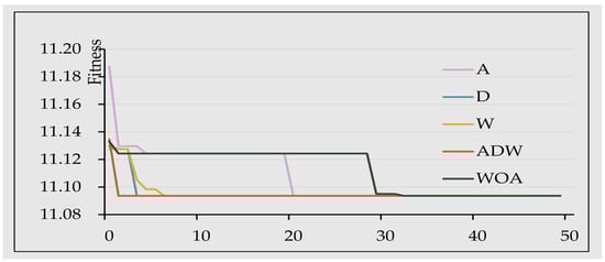
Figure 3.
Convergence curves of different strategies to optimize the whale algorithm.
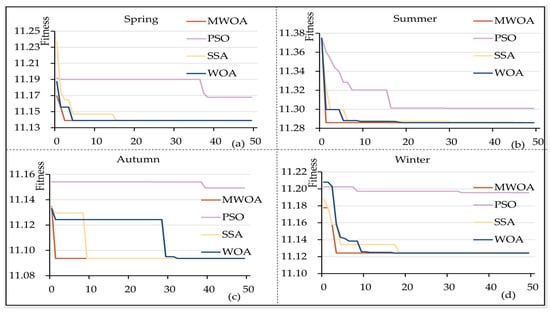
Figure 4.
Comparison of convergence curves of different optimization algorithms.
The VMD decomposition depended on the parameter choices. The penalty factor is the decomposition completeness balancing parameter, and picking adjusts the VMD method completeness. If is too high, band information is lost or redundant. The optimal parameter combination must be found since over- or under-decomposition will occur if is too big. The central frequency observation technique was currently employed to find the value by monitoring the central frequency under numerous values of , but it could only detect the number of formats and not the penalty parameter . This coefficient’s usual range is 1000–3000, and its general value is 2000.
Table 4 displays the results of the central frequency approach for determining the values [32] and the VMD decomposition using the MWOA whale optimization algorithm for the four seasons. Comparing the experimental findings of utilizing the central frequency domain approach to identify the decomposition number of VMD with the experimental results of the MWOA optimization algorithm revealed a superior prediction accuracy in Table 5.
Table 4.
Decomposition results of the VMD.
Table 5.
Evaluation of the effectiveness of the MWOA-optimized VMD in real power plants.
4.4. Experiment I: Evaluate and Compare Common Individual Models
It was possible to compare the accuracy of forecasting of the conventional system with that of the devised system in this research project. In Figure 5 we display the evaluation criteria results.
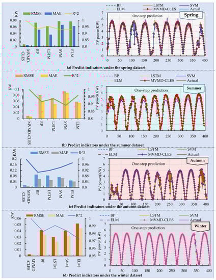
Figure 5.
Comparison of the predictive performance and simulation results of five systems.
(a) The predictive performance evaluation of the BP, LSTM, ELM, and SVM in the spring, summer, and autumn was not high, and they were susceptible to environmental changes. The fluctuation of winter weather was relatively small, and satisfactory prediction results have been achieved. The average RMSE, MAE, and R2 for the four seasons of LSTM were 0.0618 KW, 0.0403 KW, and 94.94%, respectively, while the BP model was 0.0713 KW, 0.0515 KW, and 93.50%. Using the VMD for the data smoothing processing made it have less noise interference. Due to the smaller amplitude of high-frequency components, the prediction of low-frequency components was easier, and a combined prediction model with superposition was used. The average RMSE, MAE, and R2 of the MVMD–CLES were 0.0087 KW, 0.006 KW, and 99.88%, respectively. Compared with other single models, it showed the superiority of the prediction performance in each season.
(b) In addition, most of the RMSE values in other conventional individual systems were in the range of 0.0305 KW to 0.0931 KW. From what can be seen in Table 6, these numbers were quite near to what was anticipated when the system was first conceived. With a step size of 2, the predicted result would be lower, and embodyment in the metric values would be worse. In contrast, the MVMD–CLES integrated prediction model achieved an R2 of more than 99% for different data sets, and the prediction metric R2 still reached more than 95% as the prediction step size increased. It had stronger stability and adaptability by comparison.
Table 6.
Implementation and regulation of performance across four datasets.
4.5. Experiment II: Comparison with Common Hybrid Prediction Models
Experiment I showed that the MVMD–CLES prediction system outperformed the conventional system. There are benefits to employing the decomposition technique reconstruction to analyze data for optimal prediction, which is why it has seen widespread application in time series research. A summary of the main findings from the proposed hybrid model is shown in Figure 6 and Table 7. In-depth information was provided below.
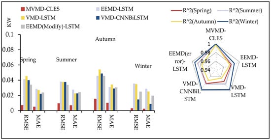
Figure 6.
The major forecast findings from Experiment II.
Table 7.
An analysis of the prediction performance of a proposed system and four mixed systems.
(a) The developed system’s forecasting efficiency was superior to that of an LSTM model based on the VMD decomposition, and the mean value of the evaluation metrics was . In addition, the VMD–LSTM predicted the best among the four winter datasets. The evaluation metrics were .
(b) Compared with the EEMD–LSTM model, in the one-step prediction, the MVMD–CLES prediction system outperformed with better mean values of the metrics , respectively. Multi-step prediction assessment metrics were better for the proposed system .
(c) In a comparison of the MVMD–CLES model to the published VMD–CNNBiLSTM [42], it was shown that the present system optimized the VMD decomposition using a multi-objective strategy whale optimization algorithm, combining the CNN, LSTM, and BiLSTM integrated networks, obtaining better metrics than the former in most data sets. The EEMD(Modify)–LSTM prediction network was constructed in combination with the constructive error correction network proposed in the literature [43]. For the one-step prediction, the mean score for each of the four data was . In the two-step prediction, they were . Compared with the comparison system, the MVMD–CLES system predicted higher. Consequently, the suggested prediction model in this work offered better potential.
4.6. Experiment III: Evaluating the Incorporation of Various Meteorological Characteristics
To facilitate comparison, this section offers historical meteorological parameters and power data. By independently incorporating meteorological factors and the PV time series time-frequency components into the same model, this study proposed a multi-branch feature extraction structure based on a stacking integration framework to compare and analyze input forms. Table 8 shows the performance of various models in all four seasons. In addition, in order to better illustrate the prediction results, further determine the effectiveness of the prediction, and measure the growth rate of the prediction. The RMSE, MAE error reduction rate, and R2 improvement rate between each model in the complete test set are shown in Figure 7. The specific calculation method is shown in Equation (27).
Table 8.
The performance of the various models across all four seasons.
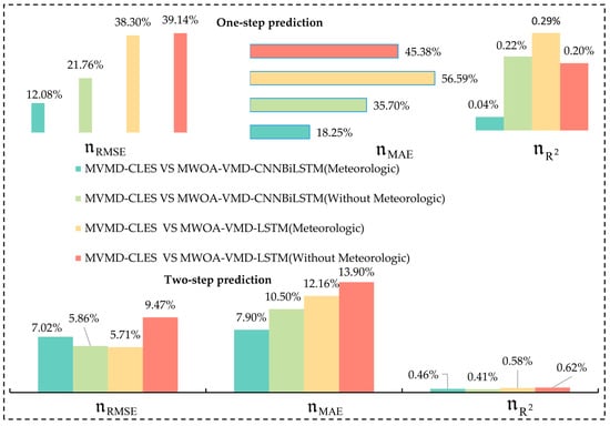
Figure 7.
The average improvement percentage of evaluation indicators.
(a) The model proposed on the basis of stacking integration of extracting meteorological factor features in each branch of the model individually outperforming the method, whether or not there were incorporated meteorological variables in the same structure. With a prediction accuracy of over 99% in all four datasets, it was proven that the designed system can fully integrate meteorological elements and environmental changes. The adaptability and flexibility were improved.
(b) Evidence suggests that the CNN convolutional network extracted meteorological features significantly, and the CNN–BiLSTM hybrid network improved the prediction effect relatively by introducing meteorological features. Although historical meteorological features were introduced, the LSTM-based network had a relatively low prediction effect; perhaps because of the incorporation of a great deal of meteorological data, which interferes with the model’s evaluation of the primary photovoltaic power information and gives rise to certain puzzling characteristics.
(c) This survey’s technique usually yielded a lower RMSE and MAE predictive performance, as seen above. The experimental findings showed that the proposed hybrid integrated deep learning model was more effective, owing to the data reconstruction for distinct time-frequency components with the VMD. While the CNN–BiLSTM and data decomposition can extract intrinsic and periodic characteristics, meteorological factor variables were inserted according to climatic circumstances, and the PV power and meteorological factors were modeled individually to derive characteristics. As a final note, the results of each branch were integrated by stacking, and the ELM was used as a secondary prediction model to finally obtain the forecasted outcome. This strategy enhanced the model’s forecast and eliminated weather-related fluctuations.
5. Conclusions
We developed a model MVMD–CLES that incorporated the benefits of four machine learning methods (CNN, BiLSTM, LSTM, ELM), as well as the whale optimization approach and the variational pattern decomposition method. Particularly, the variational pattern decomposition, using the multi-objective optimization method whale algorithm, would intelligently optimize the parameters and lessen the impact of noise in the signal. Prediction accuracy may be greatly enhanced by accelerating convergence and avoiding local optimum solutions. Improving the convergence speed and avoiding falling into local optimal solutions can boost forecast accuracy. The created system and other regularly used systems are also utilized as predictors to evaluate the real power station data sequences from Alice Spring, Australia, using three evaluation metrics RMSE, MAE and R2. Finally, the created system was compared to other prediction systems, and comprehension tests proved its predictive validity and stability. In summary, the following conclusions were obtained:
(1) The proposed system achieve significant accuracy in PV generation forecasting;
(2) As a result of its design, the system produced more robust and efficient forecasts than the four commonly used monolithic models and four hybrid systems used for the chosen dataset;
(3) The whale algorithm based on a multi-objective optimization strategy combined with variational modal decomposition, was an effective strategy.
(4) The stacking-based integration of the multi-branch forecasting network, which put meteorological variables and historical power data in different models. The inclusion of meteorological parameters and the anticipated variation due to weather changes were less likely to produce a disruption when using this multi-branch feature extraction method.
Therefore, in order to further improve the performance of the proposed data-driven model for the PV power generation prediction and extend its application scenarios, more efforts should be made.
Author Contributions
All of the authors contributed extensively to the work. Reviewing and software, L.L.; software, methodology, and writing—original draft preparation, K.G.; writing—review and editing, J.C.; data curation and visualization, L.G.; conceptualization, C.K.; investigation, J.L.; supervision, D.H. All authors have read and agreed to the published version of the manuscript.
Funding
This work was supported by the Natural Science Foundation of the Fujian Province (Grant No. 2022J01952). Fujian Provincial Department of Science and Technology University Industry University Research Cooperation Project (Grant No. 2022H6005).
Data Availability Statement
The data set for the experimental data in the paper can be obtained from http://dkasolarcentre.com.au/download.
Acknowledgments
Our profound appreciation goes out to the editors and reviewers whose meticulous effort and insightful comments helped make this publication stronger.
Conflicts of Interest
The authors state that they have no financial or personal ties to other parties that might potentially affect the results presented in this study.
Nomenclature
| PV | Photovoltaic |
| RF | Random forest |
| GTB | Gradient tree boosting |
| SVM | Support vector machines |
| Boost | Extreme gradient boosting |
| ML | Machine learning |
| DL | Deep learning |
| PVPF | PV power forecasting |
| ELM | Extreme learning machines |
| BP | Back propagation |
| CNN | Convolutional neural networks |
| LSTM | Long short-term memory |
| 1DCNN | One-dimensional CNN |
| 2DCNN | Two-dimensional CNN |
| EMD | Empirical mode composition |
| EEMD | Ensemble empirical mode decomposition |
| WT | Wavelet transform |
| CEEMDAN | Complete ensemble empirical mode decomposition with adaptive noise |
| GRU | Gated recurrent unit |
| VMD | Variational mode decomposition |
| PSO | Particle swarm optimization |
| SSA | Sparrow search algorithm |
| WOA | Whale optimization algorithm |
| MWOA | Multi-strategy whale optimization algorithm |
| KELM | Kernel-based extreme learning machine |
| IMFs | Intrinsic mode functions |
| MAE | Mean absolute error |
| NWP | Numerical weather parameter |
| RMSE | Root mean square error |
| RH | Relative humidity |
| Temp | Temperature |
| GHI | Global horizontal irradiance |
| DHI | Direct horizontal irradiance |
| WS | Wind speed |
| MVMD–CLES | CNN–LSTM–ELM stacking with MWOA-optimized VMD |
References
- Wang, F.; Xuan, Z.; Zhen, Z.; Li, K.; Wang, T.; Shi, M. A day-ahead PV power forecasting method based on LSTM-RNN model and time correlation modification under partial daily pattern prediction framework. Energy Convers. Manag. 2020, 212, 112766. [Google Scholar] [CrossRef]
- Luo, X.; Zhang, D. An adaptive deep learning framework for day-ahead forecasting of photovoltaic power generation. Sustain. Energy Technol. Assess. 2022, 52, 102326. [Google Scholar] [CrossRef]
- Ahmed, R.; Sreeram, V.; Togneri, R.; Datta, A.; Arif, M.D. Computationally expedient Photovoltaic power Forecasting: A LSTM ensemble method augmented with adaptive weighting and data segmentation technique. Energy Convers. Manag. 2022, 258, 115563. [Google Scholar] [CrossRef]
- Chen, J.; Zhang, N.; Liu, G.; Guo, L.; Li, J. Photovoltaic short-term output power forecasting based on EOSSA-ELM. Renew. Energy 2022, 40, 890–898. [Google Scholar] [CrossRef]
- Singh, S.N.; Mohapatra, A. Repeated wavelet transform based ARIMA model for very short-term wind speed forecasting. Renew. Energy 2019, 136, 758–768. [Google Scholar] [CrossRef]
- Etxegarai, G.; López, A.; Aginako, N.; Rodríguez, F. An analysis of different deep learning neural networks for intra-hour solar irradiation forecasting to compute solar photovoltaic generators’ energy production. Energy Sustain. Dev. 2022, 68, 1–17. [Google Scholar] [CrossRef]
- Hu, K.; Li, Y.; Jiang, X.; Li, J.; Hu, Z. Application of Improved Neural Network Model in Photovoltaic Power Generation. Comput. Syst. Appl. 2019, 28, 37–46. [Google Scholar] [CrossRef]
- Ramos, L.; Colnago, M.; Casaca, W. Data-driven analysis and machine learning for energy prediction in distributed photovoltaic generation plants: A case study in Queensland, Australia. Energy Rep. 2022, 8, 745–751. [Google Scholar] [CrossRef]
- Leme, J.V.; Casaca, W.; Colnago, M.; Dias, M.A. Towards Assessing the Electricity Demand in Brazil: Data-Driven Analysis and Ensemble Learning Models. Energies 2020, 13, 1407. [Google Scholar] [CrossRef]
- Leva, S.; Dolara, A.; Grimaccia, F.; Mussetta, M.; Ogliari, E. Analysis and validation of 24 hours ahead neural network forecasting of photovoltaic output power. Math. Comput. Simul. 2017, 131, 88–100. [Google Scholar] [CrossRef]
- Markovics, D.; Mayer, M.J. Comparison of machine learning methods for photovoltaic power forecasting based on numerical weather prediction. Renew. Sustain. Energy Rev. 2022, 161, 112364. [Google Scholar] [CrossRef]
- Andrade, J.R.; Bessa, R.J. Improving Renewable Energy Forecasting with a Grid of Numerical Weather Predictions. IEEE Trans. Sustain. Energy 2017, 8, 1571–1580. [Google Scholar] [CrossRef]
- Wang, H.; Lei, Z.; Zhang, X.; Zhou, B.; Peng, J. A review of deep learning for renewable energy forecasting. Energy Convers. Manag. 2019, 198, 111799. [Google Scholar] [CrossRef]
- Wang, J.; Jiang, H.; Wu, Y.; Dong, Y. Forecasting solar radiation using an optimized hybrid model by Cuckoo Search algorithm. Energy 2015, 81, 627–644. [Google Scholar] [CrossRef]
- Behera, M.K.; Majumder, I.; Nayak, N. Solar photovoltaic power forecasting using optimized modified extreme learning machine technique. Eng. Sci. Technol. Int. J. 2018, 21, 428–438. [Google Scholar] [CrossRef]
- Eseye, A.T.; Zhang, J.; Zheng, D. Short-term photovoltaic solar power forecasting using a hybrid Wavelet-PSO-SVM model based on SCADA and Meteorological information. Renew. Energy 2018, 118, 357–367. [Google Scholar] [CrossRef]
- Liu, L.; Liu, D.; Sun, Q.; Li, H.; Wennersten, R. Forecasting Power Output of Photovoltaic System Using A BP Network Method. Energy Procedia 2017, 142, 780–786. [Google Scholar] [CrossRef]
- An, W.; Zheng, L.; Yu, J.; Wu, H. Ultra-short-term prediction method of PV power output based on the CNN–LSTM hybrid learning model driven by EWT. J. Renew. Sustain. Energy 2022, 14, 053501. [Google Scholar] [CrossRef]
- Gao, M.; Li, J.; Hong, F.; Long, D. Day-ahead power forecasting in a large-scale photovoltaic plant based on weather classification using LSTM. Energy 2019, 187, 115838. [Google Scholar] [CrossRef]
- Li, J.; Song, Z.; Wang, X.; Wang, Y.; Jia, Y. A novel offshore wind farm typhoon wind speed prediction model based on PSO–Bi-LSTM improved by VMD. Energy 2022, 251, 123848. [Google Scholar] [CrossRef]
- Han, M.; Zhong, J.; Sang, P.; Liao, H.; Tan, A. A Combined Model Incorporating Improved SSA and LSTM Algorithms for Short-Term Load Forecasting. Electronics 2022, 11, 1835. [Google Scholar] [CrossRef]
- Yu, M.; Niu, D.; Wang, K.; Du, R.; Yu, X.; Sun, L.; Wang, F. Short-term photovoltaic power point-interval forecasting based on double-layer decomposition and WOA-BiLSTM-Attention and considering weather classification. Energy 2023, 275, 127348. [Google Scholar] [CrossRef]
- Miao, D.; Ji, J.; Chen, X.; Lv, Y.; Liu, L.; Sui, X. Coal and Gas Outburst Risk Prediction and Management Based on WOA-ELM. Appl. Sci. 2022, 12, 10967. [Google Scholar] [CrossRef]
- Agga, A.; Abbou, A.; Labbadi, M.; Houm, Y.E.; Ali, I.H. CNN-LSTM: An efficient hybrid deep learning architecture for predicting short-term photovoltaic power production. Electr. Power Syst. Res. 2022, 208, 107908. [Google Scholar] [CrossRef]
- He, Y.; Gao, Q.; Jin, Y.; Liu, F. Short-term photovoltaic power forecasting method based on convolutional neural network. Energy Rep. 2022, 8, 54–62. [Google Scholar] [CrossRef]
- Lin, W.; Zhang, B.; Li, H.; Lu, R. Multi-step prediction of photovoltaic power based on two-stage decomposition and BILSTM. Neurocomputing 2022, 504, 56–67. [Google Scholar] [CrossRef]
- Gao, B.; Huang, X.; Shi, J.; Tai, Y.; Zhang, J. Hourly forecasting of solar irradiance based on CEEMDAN and multi-strategy CNN-LSTM neural networks. Renew. Energy 2020, 162, 1665–1683. [Google Scholar] [CrossRef]
- Wang, R.; Li, C.; Fu, W.; Tang, G. Deep Learning Method Based on Gated Recurrent Unit and Variational Mode Decomposition for Short-Term Wind Power Interval Prediction. IEEE Trans. Neural Netw. Learn. Syst. 2019, 31, 3814–3827. [Google Scholar] [CrossRef]
- Abdelmoula, I.A.; Elhamaoui, S.; Elalani, O.; Ghennioui, A.; Aroussi, M.E. A photovoltaic power prediction approach enhanced by feature engineering and stacked machine learning model. Energy Rep. 2022, 8, 1288–1300. [Google Scholar] [CrossRef]
- Khan, W.; Walker, S.; Zeiler, W. Improved solar photovoltaic energy generation forecast using deep learning-based ensemble stacking approach. Energy 2022, 240, 122812. [Google Scholar] [CrossRef]
- Li, Z.; Xu, R.; Luo, X.; Cao, X.; Du, S.; Sun, H. Short-term photovoltaic power prediction based on modal reconstruction and hybrid deep learning model. Energy Rep. 2022, 8, 9919–9932. [Google Scholar] [CrossRef]
- Chen, X.; Ding, K.; Zhang, J.; Han, W.; Liu, Y.; Yang, Z.; Weng, S. Online prediction of ultra-short-term photovoltaic power using chaotic characteristic analysis, improved PSO and KELM. Energy 2022, 248, 123574. [Google Scholar] [CrossRef]
- Zhang, C.; Peng, T.; Nazir, M.S. A novel integrated photovoltaic power forecasting model based on variational mode decomposition and CNN-BiGRU considering meteorological variables. Electr. Power Syst. Res. 2022, 213, 108796. [Google Scholar] [CrossRef]
- Mellit, A.; Pavan, A.M.; Lughi, V. Deep learning neural networks for short-term photovoltaic power forecasting. Renew. Energy 2021, 172, 276–288. [Google Scholar] [CrossRef]
- Huang, H.; Yan, Q. Data Processing Method of Bridge Deflection Monitoring Based on WOA-VMD. Sci. Technol. Innov. 2022, 31, 118–121. [Google Scholar]
- Ni, A.; Wang, Y.; Xue, H. A Method to Forecast Ultra-Short-Term Output of Photovoltaic Power Generation Based on Chaotic Characteristic-Improved Whale Optimization Algorithm and Relevance Vector Machine. Mod. Electr. Power 2021, 38, 268–276. [Google Scholar] [CrossRef]
- Zhou, J.; Xiao, M.; Niu, Y.; Ji, G. Rolling Bearing Fault Diagnosis Based on WGWOA-VMD-SVM. Sensors 2022, 22, 6281. [Google Scholar] [CrossRef]
- Tang, P.; Chen, D.; Hou, Y. Entropy method combined with extreme learning machine method for the short-term photovoltaic power generation forecasting. Chaos Solitons Fractals 2016, 89, 243–248. [Google Scholar] [CrossRef]
- Zhen, H.; Niu, D.; Wang, K.; Shi, Y.; Ji, Z.; Xu, X. Photovoltaic power forecasting based on GA improved Bi-LSTM in microgrid without meteorological information. Energy 2021, 231, 120908. [Google Scholar] [CrossRef]
- [Dataset] Desert Knowledge Australia Centre. Download Data. Location (e.g. Alice Springs). Available online: http://dkasolarcentre.com.au/download (accessed on 22 February 2023).
- Tang, D.; Zhu, W.; Hou, L. Ultra-short-term photovoltaic power prediction based on CNN-LSTMXGBoost model. Chin. J. Power Sources 2022, 46, 1048–1052. [Google Scholar]
- Neshat, M.; Nezhad, M.M.; Sergiienko, N.Y.; Mirjalili, S.; Piras, G.; Garcia, D.A. Wave power forecasting using an effective decomposition-based convolutional Bi-directional model with equilibrium Nelder-Mead optimizer. Energy 2022, 256, 124623. [Google Scholar] [CrossRef]
- Wang, R.; Ran, F.; Lu, J. Wind Power Prediction Based on Run Discriminant Method and VMD Residual Correction. J. Hunan Univ. (Nat. Sci.) 2022, 49, 128–137. [Google Scholar] [CrossRef]


Disclaimer/Publisher’s Note: The statements, opinions and data contained in all publications are solely those of the individual author(s) and contributor(s) and not of MDPI and/or the editor(s). MDPI and/or the editor(s) disclaim responsibility for any injury to people or property resulting from any ideas, methods, instructions or products referred to in the content. |
© 2023 by the authors. Licensee MDPI, Basel, Switzerland. This article is an open access article distributed under the terms and conditions of the Creative Commons Attribution (CC BY) license (https://creativecommons.org/licenses/by/4.0/).