Flexible Load Multi-Step Forecasting Method Based on Non-Intrusive Load Decomposition

Abstract

Accurate forecasting of flexible loads can capture the potential of their application and improve the adjustable space of the distribution network. Flexible load data, such as air conditioning (AC) and electric vehicles (EV), are generally included in the total load data, making it difficult to forecast them directly. To this end, this paper proposes a multi-step flexible load prediction model based on the non-intrusive load decomposition technique and Informer algorithm. The CNN-BiLSTM model is first used to decompose the flexible load from the total load via feature extraction and feature mapping of the flexible load to the overall load. The Informer model is then used to predict the flexible load and the residual load separately in multiple steps, and the prediction results are summed to obtain the overall prediction results. In this paper, the model is validated using two datasets, where in dataset 1, the prediction coefficients of determination for flexible load air conditioning and electric vehicles are 0.9329 and 0.9892. The predicted value of the total load is obtained by adding the flexible load to the residual load. At a prediction step of 1, the total load prediction coefficient of determination is 0.9813, which improves the prediction coefficient of determination by 0.0069 compared to the direct prediction of the total load, and prediction decision coefficient improves by 0.067 at 20 predicted steps. When applied to data set 2, the prediction coefficient of determination for flexible load air conditioning is 0.9646.

1. Introduction

With the development of economy and society, the trend of seasonal and periodical shortages of power supply has become normalized, the problem of energy supply security is becoming more and more prominent, and it has become increasingly important to alleviate the contradiction between the supply and demand sides [1]. The scheduling and regulation of flexible loads can effectively alleviate the contradiction between supply and demand, which is an important means of securing power supply [2]. The forecasting of flexible loads can predict the adjustable space of flexible loads in advance, which is of great significance to provide relief from supply and demand-side conflicts [3].

Air conditioners [4], electric vehicles [5], etc., are typical flexible loads whose data are generally included in the overall customer load data and cannot be predicted directly. Influenced by weather, time, electricity price, incentive policies, and realistic demand [6,7,8], flexible loads are highly volatile and random, which also affects the prediction accuracy of the overall load. Therefore, it is practical to decompose the flexible load from the total load and then make predictions; however, there are few prediction research results for flexible load.

There are two existing load disaggregation methods: intrusive load monitoring (ILM) and non-intrusive load monitoring (NILM). The ILM method installs a separate sensor for each load, eliminating the load disaggregation step and allowing access to accurate energy consumption information for each load. However, the method requires the installation of sensors for each load of each occupant or building, which is time-consuming and labor-intensive when conducting the rollout. Additionally, the ILM method interferes with the normal life of users and involves user privacy issues when collecting data. The NILM method only needs to add a power meter to the main electrical panel of each user or building, which does not disturb the occupants during data collection. By simply installing a single power meter for the whole floor or building to obtain the overall load data of the user or building, through the load decomposition algorithm, the energy consumption information of each load can be obtained. With the continuous development of machine learning, the load decomposition accuracy of decomposition is rising, and therefore the NILM method is widely used [9].

This paper proposes the use of the load decomposition technique to extract the flexible load from the total load, retain the flexible load characteristics, obtain the data sample set of the flexible load, and then perform flexible load prediction based on the flexible load data sample set.

The current non-invasive load decomposition (NILD) technique possesses high accuracy [10,11,12,13,14,15,16,17,18,19], but the flexible load state is variable and the power threshold changes, and the traditional decomposition method requires event detection, which is not applicable to flexible load decomposition [10,11]. Deep-learning-based methods, which do not require event detection, improve the accuracy of flexible load decomposition by performing feature extraction and feature mapping of the target load to the overall load [12,13,14]. For feature extraction, graph signal processing theory [15], fast Fourier transform [16], and spectral map theory are mostly used, which can extract load features to a certain extent but cannot distinguish multi-state loads. In this paper, a one-dimensional convolutional neural network (CNN) is adopted for feature extraction, and CNN can effectively extract the deep-level features embedded in the data with reduced algorithm complexity. In terms of feature mapping, the bi-directional long short-term neural network (BiLSTM) overcomes the drawback of the long short-term memory neural network (LSTM) network only being able to perform one-way learning, and improves the feature mapping effect through bi-directional learning [19].

Combinatorial prediction models are the current hotspot in load prediction, which generally use wavelet decomposition [20], empirical modal decomposition [21], variational modal decomposition [22], and complete ensemble empirical modal decomposition to decompose the load sequence into multiple components to reduce the load nonlinearity, and then use LSTM, BiLSTM, and other methods for prediction. This type of method is based on single-step prediction, and the accuracy of multi-step prediction is poor, which is not suitable for the actual demand of scheduling. Meanwhile, this combined prediction method is prone to data leakage when performing sequence decomposition [23].

Compared with traditional deep learning, CNN, LSTM, etc., transformer models can capture long-range dependencies between time series more effectively, support parallel training of the model, and have better model performance [24], which is mostly used in language recognition, text recognition, etc. Informer model is an improvement based on a transformer model, in which a self-attention mechanism with the addition of probabilistic sparsification, which not only can avoid the recursive transmission between information and effectively capture the effective information between sequences [25], but also reduces the complexity in the temporal sequence, improves the prediction accuracy and efficiency, and is more suitable for prediction of temporal data. The method does not have a data leakage problem and performs better in multi-step prediction.

In summary, this paper proposes a two-stage flexible load prediction method based on non-intrusive decomposition technique. In the first stage, the corresponding data are collected according to the smart meters on the customer side, a deep learning model based on CNN-BiLSTM is constructed using a non-intrusive load decomposition technique, the CNN method is used to obtain the flexible load features, and the BiLSTM method is used to perform flexible load feature mapping to accurately decompose the flexible load from the total load. In the second stage, the Informer model is used to perform multi-step flexible load prediction based on the sample set of flexible load data decomposed in the first step. Finally, the method of this paper is applied to a regional electricity load data set, and the results show that the model of this paper can decompose the flexible load from the total load, retain the change characteristics of the flexible load, and realize the future prediction of the flexible load and the residual load, respectively, and the prediction accuracy of Informer is significantly improved compared with the traditional prediction model when multi-step prediction is performed, and the more the number of prediction steps, the more obvious the improvement is. In this paper, the model is validated using two datasets, where dataset 1, the prediction coefficients of determination for flexible load air conditioning and electric vehicles, are 0.9329 and 0.9892. The predicted value of the total load is obtained by adding the flexible load to the residual load. At a prediction step of 1, the total load prediction coefficient of determination is 0.9813, which improves the prediction coefficient of determination by 0.0069 compared to the direct prediction of the total load, and prediction decision coefficient improves by 0.067 at 20 predicted steps. When applied to data set 2, the prediction coefficient of determination for flexible load air conditioning is 0.9646.

2. Non-Intrusive Load Decomposition

2.1. Principle of Decomposition

The non-intrusive load decomposition is actually a decomposition of the total load power sequence. The decomposition yields the power sequence of each appliance load.

A customer has $n$ loads, and when at a certain moment $t$, the total power is $P_{\mathrm{t}}$ and the power of the $i$ load is $P_{i,t}$, satisfying:

$$P_t={\displaystyle \sum _{i=1}^n{P}_{i,t}}$$

(1)

Non-invasive load decomposition using deep learning methods essentially learns the load characteristics of the individual load $P_{i,t}$ and the relationship between the total power $P_{\mathrm{t}}$ and $P_{i,t}$. The power of individual loads is then decomposed from the total load power.

2.2. Model Principle

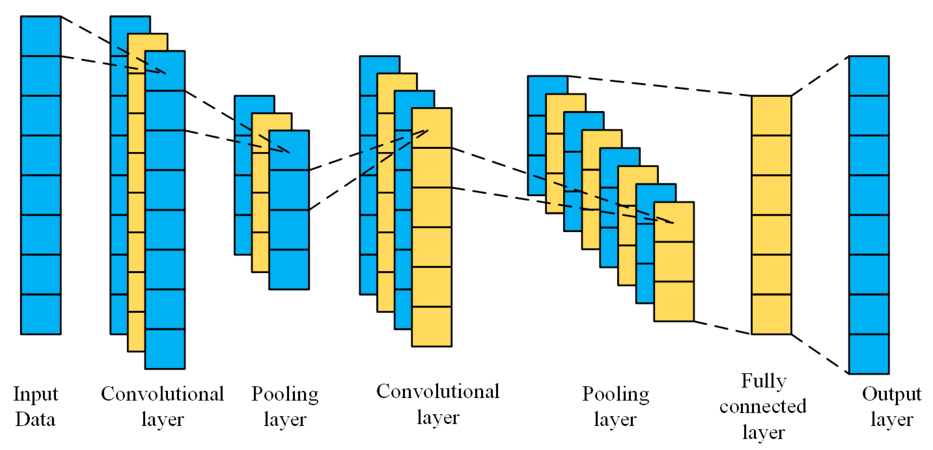
2.2.1. Convolutional Neural Network (CNN)

In this paper, a one-dimensional CNN is used to construct an end-to-end feature extraction model directly. Figure 1 shows a typical structural framework of a one-dimensional CNN, consisting of a series of convolutional layers, pooling layers, and fully connected layers. The convolutional layer performs convolutional computation on the data to extract potential features, and the pooling layer downsamples and compresses the network parameters. The alternating use of convolutional and pooling layers maximizes the extraction of potential features from the input data and reduces the errors caused by human operations.

2.2.2. Bi-Directional Long Short Term Memory Network (BiLSTM)

A bi-directional long short-term memory network (BiLSTM) is a combination of LSTM and bi-directional RNN, which can use the temporal information in both past and future directions for model training.

The structure of the long short-term memory unit and the way the structure is connected at moments t to t + 1 are given in Figure 2, where the components are calculated as follows:

$$E_f=\delta (W_f\ast \left[h_{t-1},x_t\right]+b_f)$$

(2)

$$E_i=\delta (W_i\ast \left[h_{t-1},x_t\right]+b_i)$$

(3)

$$C_t^{\prime }=\tanh (W_c\ast \left[h_{t-1},x_t\right]+b_c)$$

(4)

$$C_t=E_f\ast C_{t-1}+E_i\ast C_t^{\prime }$$

(5)

$$E_o=\delta (W_o\ast \left[h_{t-1},x_t\right]+b_o)$$

(6)

$$h_t=E_o\ast \tanh (C_t)$$

(7)

where $E_f$, $E_i$, and $E_o$ are the outputs of the forgetting gate, the input gate, and the output gate at time $t$, respectively; $C_t$ and $C_t^{\prime }$ are the cell state at time $t$ and the intermediate cell state; $x_t$ is the input to the hidden layer at time $t$; $h_{t-1}$ and $h_t$ are the output of the hidden layer at moment $t-1$ and moment $t$, $W_f$, $W_i$, $W$, $W_o$, $b_f$, $b_i$, $b_c$, and $b_o$ are the weights and biases for the oblivion gate, input gate, output gate, and intermediate cell states; and $\delta$ is the Sigmoid function.

The bi-directional concept is introduced on the basis of the LSTM network to obtain the features of the whole time domain. As shown in Figure 3, the model uses the forward and reverse processes to obtain past and future information in the input data $x_t$ and passes it to the output layer to obtain $y_t$ for forward and reverse training.

In RNN, as the sequence advances, the hidden states are passed backward in turn, and the gradients accumulate in the process, so it is easy to cause the problems of gradient disappearance or gradient explosion; in LSTM, the long-term information is saved in the unit state and passed backward, and the network adds the “forgetting gate” to control the gradient disappearance and gradient explosion by learning parameters. In LSTM, long-term information is stored in the cell state and passed backward, and the network adds a “forgetting gate” to control the long-term information transfer by learning parameters, thus effectively alleviating the gradient disappearance and gradient explosion problems.

2.3. Decomposition Network

The decomposition network consists of three parts: the first part is the feature extraction part, which inputs the original power sequence and the target power into the 1D convolutional layer, extracts the feature relationship between the original power sequence and the target power sequence through two 1D convolutional layers and a maximum pooling layer, and generates the feature encoding matrix; the second part is the feature learning layer, which passes the feature encoding matrix generated in the first part into the second part; the feature encoding matrix is learned through the BiLSTM layer to learn the relationship between the original power sequence and the target power sequence. The third part is the feature mapping part, which maps the output of the BiLSTM layer through a fully connected layer to obtain an output sequence of the same length as the original power sequence. The overall structure of the model is shown in Figure 4.

3. Load Forecasting Model

3.1. Principle of Informer Model

The Informer model as a whole can be divided into two parts: the encoder (Encoder) and the decoder (Decoder). The encoder extracts long-term dependencies from the original sequence input by successive distillation operations. The feature maps of interest are obtained from the long-term dependencies. The decoder predicts the output by combining the information and the feature maps. The overall model structure is shown in Figure 5:

The main input to the model is the $F$ normalized impact factor data for the previous $t$ moments: $X={\left(X_1,X_2,\cdots X_t\right)}^T\in R^{F*t}$, before input to the model, the impact factor data are first transformed from $F$ expansion to $d$ dimensionality.

For the time series prediction problem, the sequential relationship between the data is crucial. Informer encodes the position information of each input data (position embedding). With positional embedding, the positional relationships (sequential structure) are not lost after the sequence data is input to the model. The specific operation formula is shown in (8) and (9):

$$P{E}_{(pos,2j)}=\sin \frac{pos}{{(2L)}^{2j/d}}$$

(8)

$$P{E}_{(pos,2j-1)}=\cos \frac{pos}{{(2L)}^{2j/d}}$$

(9)

where $j\in \left\{1,\dots ,\frac{d}{2}\right\}$ $d$ is the number of dimensions, $pos$ is the position (sequence order), and $L$ is the length of the input sequence.

The encoder input is a long sequence from historical data (as in the first 2 h). Inside the encoder is a stack of multi-headed probabilistic sparse self-attentive modules and “distillation” mechanism modules [20]. The probabilistic sparse self-attentive mechanism is shown in Equation (10):

$$A(Q,K,V)=Soft\max (\frac{\overline{Q}{K}^T}{\sqrt{d}})V$$

(10)

where $Q,K,V$ is a matrix of query vectors, key vectors, and value vectors, respectively, and $Q,K,V$ are three matrices of the same size obtained by the linear transformation of the input eigenvariables. The self-attentive mechanism often uses the key–value–query model, which assigns a value to a key by comparing its similarity to a query. Informer lets the key focus only on the top $j$ most important queries, $\overline{Q}$ is obtained by probabilistic sparsification of $Q$, $\overline{Q}$ contains only the sparse matrix of the first u query, and $Soft\max$ is the activation function [23].

Informer uses the distilling method to assign higher weights to the dominant features with primary information. Additionally, generate the focused self-attentive feature map at j + 1 layer for the previous layer. As shown in Equation (11):

$$X_{j+1}=MaxPool(ELU(Concld{(X_j)}_{AB}))$$

(11)

This equation implements the “distillation operation” in Informer, which is essentially a one-dimensional temporal convolution, $ELU$ activation function, and maximum pooling, with ${\left(\right)}_{AB}$ representing the attention block. The purpose of the “distillation” operation is to compress the feature dimensions and extract the main information. $Concld$ denotes a one-dimensional convolution operation on the time series with $ELU$ as the activation function, and finally a $MaxPool$ layer with a step size of 2, which allows the computation of each layer to be halved and the model to retain the information of the long input time series.

The input to the decoder consists of a short sequence (e.g., the first 1 h) combined with a segment of zero values equal to the prediction compensation. Inside the decoder, the input data first undergoes a multi-headed probabilistic sparse self-attentiveness operation with Masked, and then performs a multi-headed self-attentiveness operation with the intermediate results of the encoder output, and finally adjusts the data output dimension by the fully connected layer to obtain the prediction result $Y={\left(Y_{t+1},Y_{t+2},\cdots Y_{t+n}\right)}^T$. The output prediction results are calculated as a loss function and then backward gradient propagation is performed to continuously optimize the model [24].

3.2. Forecasting Model Structure

The specific prediction process of the non-intrusive load decomposition-based load forecasting model proposed in this paper is shown in Figure 6.

Firstly, the flexible load in the original load sequence is decomposed by the non-intrusive load decomposition technique to form the flexible load curve and the residual load curve, and then the flexible load and the residual load are predicted separately in multiple steps, so that not only the accurate prediction value of the flexible load can be obtained, but also the total load prediction value can be obtained by adding it with the residual load prediction value.

4. Analysis of Algorithms

The prediction models proposed in this paper are compared with the CNN-BiLSTM [26], VMD-CNN-BiLSTM, and Informer models using commonly used evaluation metrics.

Data Normalization and Evaluation Criteria

In order to evaluate the prediction accuracy of the prediction model taken in this paper with other models, the mean square error (MSE), mean absolute error (MAE), root mean square error (RMSE), and coefficient of determination ($R^2$) are selected, where $R^2$ denotes the linear correlation between the predicted and true values of the model, and the value of this index is taken as (0, 1); when it tends to 1, this indicates that the predicted value of the model for the sample tends to be consistent with the true value. The calculation formula of each evaluation index is as follows:

$$MSE=\frac{{\displaystyle \sum _{i=1}^m{({\widehat{y}}_i-y_i)}^2}}{m}$$

(12)

$$MAE=\frac{1}{m}{\displaystyle \sum _{i=1}^m\left|{ \mathrm{y} ^}_i-y_i\right|}$$

(13)

$$RMSE=\sqrt{\frac{{\displaystyle \sum _{i=1}^m{({\widehat{y}}_i-y_i)}^2}}{m}}$$

(14)

$$R^2=1-\frac{{\displaystyle \sum _{i=1}^m({\widehat{y}}_i-y_i}{)}^2}{{\displaystyle \sum _{i=1}^m{(y_i-\frac{1}{m}{\displaystyle \sum _{i=1}^m{y}_i})}^2}}$$

(15)

where $m$ is the number of prediction points, ${\widehat{y}}_i$ is the predicted value of the model output load, and $y_i$ is the true value of the load.

The experimental data were processed by maximum–minimum normalization in the following way:

$$l^{\prime }=\frac{l-l_{\min }}{l_{\max }-l_{\min }}$$

(16)

where $l^{\prime }$ is the normalized data, $l$ is the data to be normalized, and $l_{\max }$ and $l_{\min }$ are the maximum and minimum values of the data, respectively.

5. Experimental Verification

In this paper, two datasets were selected to validate the model. In dataset one, the experimental data were obtained from the electricity consumption data of a region, and the load data include ten kinds of loads, such as air conditioners, refrigerators, computers, dishwashers, and electric cars. For dataset two, data were obtained from the REDD dataset. The REDD dataset, published by MIT, contains energy use data from six different households over a period of weeks. In this paper, we selected house6 in the REDD dataset, which includes nine types of equipment such as air conditioners, air handling units, dishwashers, and electric furnaces (the link to the REDD dataset is http://redd.csail.mit.edu/ (accessed on 21 May 2022)).

We used Python and Pytorch to build the Informer and NILD-Informer models. Two models, CNN-BiLSTM and VMD-CNN-BiLSTM, were built with Python and Tensorflow 2.0, and the NILD-Informer model proposed in this paper was compared with the other three models for validation.

5.1. Model Parameters

To ensure the rationality of the validation method, the Informer model kept the same parameters, the parameters of VMD were optimized according to the literature [27], and the CNN and BiLSTM parameters were optimized according to the minimum prediction error, as shown in

Table 1. Model parameters.

Informer		CNN-BiLSTM, VMD-CNN-BiLSTM
Encoder input sequence length	600	Number of VMD decomposition	6
Decoder start length	60	Penalty factor	100
Encoder input size	1	Number of convolution layer filters	64
Decoder input size	1	Convolution kernel size	5
Model size	512	Pooling kernel size	3
Number of heads	8	Number of neurons	32

. Detailed model parameters are shown in Figure A1 and

Table A1. Informer model parameters.

Input sequence length of Informer encoder: 600	Start token length of Informer decoder: 60	Prediction sequence length: 1 or 5 or 10 or 20
Encoder input size: 1	Decoder input size: 1	Output size: 1
Dimension of model: 512	Number of self-attended heads: 8	ProbSparse attn factor: 5
Number of encoder layers: 2	Number of decoder layers: 1	Batch size of train input data: 20
Dropout: 0.05	Activation functions: gelu	Optimizer learning rate: 0.0001

in Appendix A.

5.2. Experiment 1

The experimental data were collected for 30 days from 1 July to 30 July 2019, with a sampling interval of 6 s once, for a total of 432,000 data.

5.2.1. Load Decomposition

The load data include ten kinds of loads such as air conditioners, refrigerators, computers, dishwashers, electric cars, etc. In this paper, Python and Tensorflow 2.0 were utilized. Both constructed a non-invasive load decomposition model based on the CNN-BiLSTM network. The data from 1 to 3 July were selected for training. The data of 4 July were selected as the test set, and the electricity consumption of each load on 4 July is shown in Figure 7. The model was used to decompose the air conditioning load and the electric vehicle load from the total load. The decomposition results are shown in Figure 8, and the decomposition accuracy is shown in

Table 2. Load decomposition accuracy.

Load	${\mathit{R}}^2$	RMSE
Air Conditioning	0.987191	101.654828
Electric Vehicles	0.997382	38.932672

:

The results from Figure 7 and Figure 8 and Table 2 show that the load power of air conditioning and electric vehicles is larger, with obvious load characteristics and high decomposition accuracy. The air conditioning and electric vehicle loads were subtracted from the total load to form three types of loads: air conditioning, electric vehicle, and residual load. The following is a multi-step prediction for each of the three types of loads.

5.2.2. Prediction and Result Analysis

We decomposed and reconstructed the data from 5 to 30 July, and the data sampling interval was adjusted to once every 5 min, with a total of 7488 data. Using the data from the first 25 days for training, the last day’s data were decomposed in multiple steps, and 1, 5, 10, and 20 steps were predicted, respectively, i.e., the prediction time scales were 5 min, 10 min, 50 min, and 100 min.

5.2.3. Decomposition of Prediction Results

Figure 9 shows the prediction results for the 10-step prediction of air conditioning load and electric vehicle load, as shown in Figure 9a,b, respectively, and

Table 3. Decomposition forecast evaluation indicators.

Load	RMSE	MAE	${\mathit{R}}^2$
Air Conditioning	226.8348	74.12682	0.932912
Electric Vehicles	64.50621	6.940884	0.989217

shows the evaluation indexes for the 10-step prediction of air conditioning and electric vehicles. Results for the other prediction steps are shown in Figure A2 and Figure A3 in Appendix A.

According to the results in Figure 9, it can be seen that the method possesses high accuracy for multi-step prediction of flexible loads, with prediction decision coefficients of 0.9329 and 0.9892 for the two flexible loads, respectively.

5.2.4. Total Load Prediction Evaluation Index Results

Four models were used for 1-step, 5-step, 10-step, and 20-step prediction, and the results of total load prediction are shown in

Table 4. Model evaluation index results.

Model	RMSE				MAE				${\mathit{R}}^2$
	1-Step	5-Step	10-Step	20-Step	1-Step	5-Step	10-Step	20-Step	1-Step	5-Step	10-Step	20-Step
CNN-BiLSTM	236.21	361.67	469.09	627.67	90.32	125.23	203.84	305.13	0.9539	0.9123	0.8561	0.7282
VMD-CNN-BiLSTM	224.06	366.61	554.50	725.26	73.63	155.35	242.26	355.52	0.9663	0.9024	0.8013	0.6476
Informer	198.00	332.70	431.67	565.54	67.34	114.61	178.25	274.84	0.9744	0.9258	0.8833	0.7792
NILD-Informer	183.71	306.11	378.20	486.82	55.81	102.08	150.80	210.24	0.9813	0.9389	0.9041	0.8462

.

5.2.5. Comparative Analysis of Experimental Results

Comparing the experimental results of CNN-BiLSTM and VMD-CNN-BiLSTM, the single-step prediction accuracy of VMD-CNN-BiLSTM was stronger than that of CNN-BiLSTM model, which is because VMD reduces the complexity of loading in line with the current mainstream view. However, when multi-step prediction was performed, the addition of new data made the decomposition error of VMD larger, leading to a greater decrease in prediction accuracy and a less effective prediction than CNN-BiLSTM.

When multi-step prediction was performed, the prediction errors of all four models increased as the number of prediction steps increased. However, the Informer model had a more stable trend of increasing prediction errors. It had better performance in different prediction steps. When the number of prediction steps was 20, the Informer model reduced the prediction error by 12.41% and 9.86% compared with the CNN-BiLSTM and VMD-CNN-BiLSTM prediction models, respectively.

Comparing the results of the NILD-Informer model and the Informer model, the NILD-Informer model was able to predict the load for air conditioning and electric vehicles separately. After reconstructing the prediction results, the multi-step prediction error of the total load of the NILD-Informer model decreased the least. Among them, the NILD-Informer model prediction reduces the RMSE of prediction error by 13.92% compared with the Informer model when 20-step prediction was performed. This indicates that NILD-Informer has higher multi-step prediction accuracy, and after decomposing air conditioners and electric vehicles from the total load, the uncertainty of the load was reduced and the prediction accuracy was improved.

5.2.6. Total Load Prediction Results

The 20-step prediction results for the total load of the above four models are shown in Figure 10. From the enlarged local details, it can be seen that the prediction fit of the NILD-Informer model is the best compared to the other three models, which can be closer to the true value with less prediction error. Additionally, the NILD-Informer model was able to predict the flexible load accurately, while the other models were not.

Based on the zoomed-in local details, it can be seen that the NILD-Informer model has the best prediction fit compared to the other three models, which can be closer to the true value and has less prediction error. The NILD-Informer model could accurately predict the flexible load, but the other models could not.

5.3. Experiment 2

The data of the REDD data set house6 was selected, which includes 9 types of equipment such as air conditioners, air handling units, dishwashers, and electric stoves, and the collection time was 30 days from 19 April to 19 May 2011, with a sampling interval of 3 s, and a total of 864,000 data.

Decomposition Prediction Results

The first four days of data were used to train the decomposition model. After using the above decomposition model, the data from 23 April to 19 May were decomposed into flexible load data and residual load data, and then the data were reconstructed and the data sampling interval was adjusted to once every 5 min, with a total of 7488 data. The parameters of the decomposition and prediction model were kept consistent with Example 1.

The decomposition forecast of air conditioning load is shown in Figure 11, the forecast evaluation index is shown in

Table 5. Decomposition forecast evaluation indicators.

Load	RMSE	MAE	${\mathit{R}}^2$
Air Conditioning	111.3321	36.61094	0.964581

, and the total load forecast result is shown in Figure 12. Results for the other prediction steps are shown in Figure A4 and Figure A5 in Appendix A

Based on the above results, it can be seen that applying this paper’s model to the REDD dataset possesses high accuracy in the decomposition prediction of flexible load air conditioning, which is beneficial for flexible loads to join the grid regulation for peak and valley reduction. The zoomed-in results in Figure 12 show that NILD-Informer has a better fit compared to the other three models. The predicted values are closer to the true values with the smallest prediction errors.

6. Conclusions

Most of the existing load forecasting methods directly predict the total load power of the power system. The problem of individual load characteristics is ignored. To address this problem, a NILD-Informer multi-step prediction model based on a non-intrusive load decomposition technique is proposed. The flexible load is decomposed from the total load for prediction, the load characteristics of the flexible load can be obtained, and the prediction accuracy of the total load is further improved.

The model proposed in this paper targets the flexible load decomposition prediction for a single user. The follow-up work focuses on verifying the extensibility of the model proposed in this paper. The object of the model becomes the whole building or community to make the model more relevant to real life. After the flexible load data are obtained from non-intrusive load decomposition, time series clustering will be performed. The electricity consumption characteristics of the whole building or community are analyzed, and the main characteristics are screened for load prediction to make buildings or communities more involved in grid regulation.

References

1. Wang, B.; Yang, Z.; Pham, T.L.H.; Deng, N.; Du, H. Can social impacts promote residents’ pro-environmental intentions and behaviour: Evidence from large-scale demand response experiment in China. Appl. Energy 2023, 340, 121031. [Google Scholar] [CrossRef]
2. Li, P.; Li, F.; Song, X.; Zhang, G. Rotational reserve optimization of new energy access system considering flexible load. Power Grid Technol. 2021, 45, 7. [Google Scholar]
3. Chan, S.H.; Ngan, H.W.; Chow, W.L. A flexible load forecasting model for integrated resources planning. In Proceedings of the DRPT2000. International Conference on Electric Utility Deregulation and Restructuring and Power Technologies, Proceedings (Cat. No.00EX382), London, UK, 4–7 April 2000; IEEE: Piscataway, NY, USA, 2000; pp. 562–565. [Google Scholar]
4. Chen, Y.; Fu, G.; Liu, X. Air-conditioning load forecasting for prosumer based on meta ensemble learning. IEEE Access 2020, 8, 123673–123682. [Google Scholar] [CrossRef]
5. Cui, J.; Liu, S.; Yang, J.; Ge, W.; Zhou, X.; Wang, A. A load combination prediction algorithm considering flexible charge and discharge of electric vehicles. In Proceedings of the 2019 IEEE 10th International Symposium on Power Electronics for Distributed Generation Systems (PEDG), Xi’an, China, 3–6 June 2019; IEEE: Piscataway, NY, USA, 2019; pp. 711–716. [Google Scholar]
6. Wang, J.; Du, C. Short-term load forecasting model based on Attention-BiLSTM neural network and meteorological data correction. Power Autom. Equip. 2022, 42, 7. [Google Scholar]
7. Karsaz, A.; Mashhadi, H.R.; Eshraghnia, R. Cooperative co-evolutionary approach to electricity load and price forecasting in deregulated electricity markets. In Proceedings of the IEEE Power India Conference, New Delhi, India, 10–12 April 2006. [Google Scholar]
8. Li, P.; He, S.; Han, P.; Zheng, M.; Huang, M.; Sun, J. Short-term load forecasting of smart grid based on long-short-term memory recurrent neural networks in condition of real-time electricity price. Power Syst. Technol. 2018, 42, 4045–4052. (In Chinese) [Google Scholar]
9. Chen, T.; Qin, H.; Li, X.; Wan, W.; Yan, W. A Non-Intrusive Load Monitoring Method Based on Feature Fusion and SE-ResNet. Electronics 2023, 12, 1909. [Google Scholar] [CrossRef]
10. Hamdi, M.; Messaoud, H.; Bouguila, N. A new approach of electrical appliance identification in residential buildings. Electr. Power Syst. Res. 2020, 178, 106037. [Google Scholar] [CrossRef]
11. Sethom, H.; Ben’S, H. Statistical Assessment of Abrupt Change Detectors for Non Intrusive Load Monitoring. In Proceedings of the 2018 IEEE International Conference on Industrial Technology (ICIT), Lyon, France, 20–22 February 2018; IEEE: Piscataway, NY, USA, 2018. [Google Scholar]
12. Yan, X.; Zhai, S.; Wang, Z.; Wang, F.; He, G. Application of Deep Neural Network in Non-intrusive Load Disaggregation. Autom. Electr. Power Syst. 2019, 43, 8. [Google Scholar]
13. Fang, Y.; Jiang, S.; Fang, S.; Gong, Z.; Xia, M.; Zhang, X. Non-Intrusive Load Disaggregation Based on a Feature Reused Long Short-Term Memory Multiple Output Network. Buildings 2022, 12, 1048. [Google Scholar] [CrossRef]
14. Xia, M.; Liu, W.; Wang, K.; Zhang, X.; Xu, Y. Non-intrusive load disaggregation based on deep dilated residual network. Electr. Power Syst. Res. 2019, 170, 277–285. [Google Scholar] [CrossRef]
15. He, K.; Stankovic, L.; Liao, J.; Stankovic, V. Non-Intrusive Load Disaggregation using Graph Signal Processing. IEEE Trans. Smart Grid 2018, 9, 1739–1747. [Google Scholar] [CrossRef] [Green Version]
16. Lin, Y.; Tsai, M. Development of an Improved Time–Frequency Analysis-Based Nonintrusive Load Monitor for Load Demand Identification. IEEE Trans. Instrum. Meas. 2014, 63, 1470–1483. [Google Scholar] [CrossRef]
17. Ma, H.; Jia, J.; Yang, X.; Zhu, W.; Zhang, H. MC-NILM: A Multi-Chain Disaggregation Method for NILM. Energies 2021, 14, 4331. [Google Scholar] [CrossRef]
18. Feng, R.; Yuan, W.; Ge, L.; Ji, S. Nonintrusive Load Disaggregation for Residential Users Based on Alternating Optimization and Down sampling. IEEE Trans. Instrum. Meas. 2021, 70, 9005312. [Google Scholar] [CrossRef]
19. Zhou, X.; Feng, J.; Li, Y. Non-intrusive load decomposition based on CNN-LSTM hybrid deep learning model. Energy Rep. 2021, 7, 5762–5771. [Google Scholar] [CrossRef]
20. Li, B.; Zhang, J.; He, Y.; Wang, Y. Short-term load-forecasting method based on wavelet decomposition with second-order gray neural network model combined with ADF test. IEEE Access 2017, 5, 16324–16331. [Google Scholar] [CrossRef]
21. Deng, D.; Li, J.; Zhang, Z.; Teng, Y.; Huang, Q. Short-term Electric Load Forecasting Based on EEMD-GRU-MLR. Power Syst. Technol. 2020, 44, 227–236. [Google Scholar]
22. Zhi, L.; Guoqiang, S.; Hucheng, L.; Zhinong, W.; Haixiang, Q.; Yizhou, Z.; Shuang, C. Short-Term Load Forecasting Based on VMD and PSO Optimized Deep Belief Network. Power Syst. Technol. 2018, 42, 598–606. [Google Scholar]
23. Qian, Z.; Pei, Y.; Zareipour, H.; Chen, N. A review and discussion of decomposition-based hybrid models for wind energy forecasting applications. Appl. Energy 2019, 235, 939–953. [Google Scholar] [CrossRef]
24. Vaswani, A.; Shazeer, N.; Parmar, N.; Uszkoreit, J.; Jones, L.; Gomez, A.N.; Kaiser, Ł.; Polosukhin, I. Attention is all you need. Adv. Neural Inf. Process. Syst. 2017, 30. [Google Scholar] [CrossRef]
25. Zhou, H.; Zhang, S.; Peng, J.; Zhang, S.; Li, J.; Xiong, H.; Zhang, W. Informer: Beyond efficient transformer for long sequence time-series forecasting. In Proceedings of the AAAI Conference on Artificial Intelligence, Vancouver, BC, Canada, 2–9 February 2021; Volume 35, pp. 11106–11115. [Google Scholar]
26. Zhu, M.; Xie, J. Investigation of nearby monitoring station for hourly PM2. 5 forecasting using parallel multi-input 1D-CNN-biLSTM. Expert Syst. Appl. 2023, 211, 118707. [Google Scholar] [CrossRef]
27. Zhang, S.; Li, J.; Jiang, A.; Huang, J.; Liu, H.; Ai, H. New two-stage short-term power load forecasting based on FPA-VMD and BiLSTM neural network. Grid Technol. 2022, 46, 3269–3279. [Google Scholar] [CrossRef]
Figure 1. D CNN network structure diagram.
Electronics 12 02842 g001
Figure 2. Structure and connection mode of short-term and long-term memory units.
Electronics 12 02842 g002
Figure 3. Structure diagram of bidirectional RNN.
Electronics 12 02842 g003
Figure 4. Load decomposition network.
Electronics 12 02842 g004
Figure 5. Informer model structure.
Electronics 12 02842 g005
Figure 6. Load forecasting model.
Electronics 12 02842 g006
Figure 7. Power consumption of each load.
Electronics 12 02842 g007
Figure 8. Load decomposition results. (a) Air conditioning load decomposition results. (b) Electric vehicle load decomposition results. (c) Residual load decomposition results.
Electronics 12 02842 g008
Figure 9. Decomposition forecast results. (a) Prediction results of air conditioning. (b) Prediction results of electric vehicles.
Electronics 12 02842 g009
Figure 10. Total load forecast results.
Electronics 12 02842 g010
Figure 11. Prediction results of air conditioning.
Electronics 12 02842 g011
Figure 12. Comparison of different models for total load.
Electronics 12 02842 g012