Abstract
Based on our previous work on the propagation of electromagnetic waves in a layered medium placed in a rectangular waveguide, we present the theory of using the TE10 and TM11 modes to determine the complex parameters of isotropic and anisotropic media. The Nicolson–Ross–Weir method was used. The cases of isotropic, uniaxial, and biaxial materials were considered. It has been shown that the TM11 mode can be used to extract parameters of non-magnetic uniaxial anisotropy media by a single measurement, without changing the sample position. This is not possible with the previously used TE10 mode. It is also possible to use the TM11 mode to quickly determine whether a material is isotropic or not. Experimental results are presented for some isotropic materials.
1. Introduction
One of the most important methods for determining the relative permittivity εr and relative permeability μr of isotropic media is the Nicolson–Ross–Weir (NRW) method. In 1970, Nicolson and Ross [1] gave the formulas for the retrieval of the electromagnetic (EM) parameters from measurements of the scattering matrix elements S11 and S21. The material under test (MUT) was placed in a coaxial transverse electromagnetic (TEM) waves transmission line. In 1974, Weir [2] obtained analogous relations for the MUT placed in a rectangular waveguide. In both works, the field reflection coefficient Γ at the interface, and the propagation coefficient P, were used. The algebraic inversion procedure used in the NRW method allows us to obtain εr and μr in terms of S11 and S21.
The overview of the NRW method and closed-form extraction equations for isotropic media can be found anywhere (see e.g., [3]). The NRW method is still being used and improved [4,5,6,7,8,9,10,11,12,13,14], in particular for the determination of the effective parameters of metamaterials (MM).
The above-mentioned methods use only a TEM mode (coaxial transmission line systems, and free-space systems), or TE modes (usually TE10 in rectangular waveguide systems). To the best of our knowledge, TM modes have not been effectively used.
Relatively little work exists that relates to methods of retrieving EM properties of anisotropic media [15,16,17,18,19,20,21,22,23]. Isotropy and anisotropy relate to the directional properties of permittivity and permeability of the media (forming crystallographic systems). Consider the so-called linear media. Using the Einstein summation convention, the relationship between the components Di (i = x, y, z) electric flux density, and Ek (k = x, y, z) electric field vectors is Di = ε0εikEk. The tensor εik is the relative permittivity tensor, and ε0 is the permittivity of vacuum. If the properties of the medium do not depend on the direction of the vector of the electric field, then such a medium is isotropic. Then, the permittivity tensor can be always written in diagonal form εik = εrδik, where δik is the Kronecker delta.
In the general case, the properties of the medium may depend on the direction; then, such a medium is called anisotropic, and the permittivity tensor has nine components. One can find eigenvalues and eigenvectors of the coordinate system in which this tensor can be represented by a diagonal matrix. Normalized eigenvectors are unit vectors defining the directions of the main axes of the crystallographic system. For three different eigenvalues, such a medium is called biaxial. When two eigenvalues of the tensor are equal, such a medium is called uniaxial. Similar considerations can be carried out for the permittivity tensor μik (see our previous work [24]). If μik = δik, then we say that the medium is non-magnetic and, in general, we are dealing only with electrical isotropy or anisotropy.
Many of the MMs realized so far are assumed to be biaxially or uniaxially anisotropic. Some conventional materials, i.e., double-positive MM, are also anisotropic.
Based on [24] on the propagation of electromagnetic waves in a layered medium placed in a rectangular waveguide, the theory of using TE10 and TM11 modes to determine the complex parameters of anisotropic and isotropic media is presented. The Nicolson–Ross–Weir method was used. The main aim of the work is to present the method. The cases of isotropic, uniaxial, and biaxial materials were considered.
The second section of the paper presents the above-mentioned theoretical basis of material parameter extraction in terms of the possibility of using the TM11 mode. To facilitate the use of the formulas for specialists who are closer to the network description, rather than the field description (see e.g., our work [24]), a graph of the signal flow for TE and TM waves, and an anisotropic structure placed in a rectangular waveguide were used. A similar approach was used by Nicolson and Ross [1] for TEM waves in a coaxial line. Although the results for the anisotropic medium, when the main axes of the crystallographic system are oriented parallel to the edges of the waveguide, are identical to those of [1] for the isotropic medium, the physical basis is fundamentally different.
The third section contains a diagram of the proposed measuring system and its practical implementation. The advantage of this configuration is the constant position of the sample in the waveguide. At the end of the chapter, the S-parameter measurements for selected frequencies and the resulting calculations are presented. These results, for isotropic media with known electromagnetic parameters, confirm the theoretical assumptions presented in the second section.
The fourth section presents the advantages of the method used, compared to traditional methods using the TE10 (or TEM) mode.
2. Extraction Procedure
2.1. Description of the Configurations
Consider the anisotropic slab of thickness d placed inside a rectangular waveguide with the cross-sectional dimensions a and b. The principal axes of the crystallographic system and the Cartesian system are oriented parallel to the waveguide edges (Figure 1), and the matrices of relative permeability ε and relative permittivity μ tensors of the medium are diagonal:
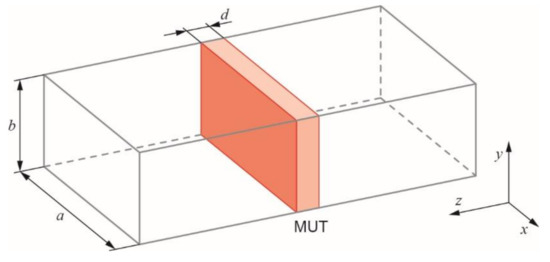
Figure 1.
A slab of thickness d placed in an air-filled rectangular waveguide with cross-sectional dimensions a and b.
Due to the possibility of using TM modes (in particular, the TM11 mode) for the extraction of material parameters, it is convenient to distinguish two configurations: that which TM waves can propagate (A), and that for which this does not occur (B).
The first case occurs when the medium is isotropic (εx = εy = εz = εr, μx = μy = μz = μr) or uniaxially anisotropic with a special configuration of MUT (εx = εy ≠ εz, μx = μy ≠ μz), so-called transversely isotropic. In this case, TM and TE waves can propagate. For an isotropic sample, two material parameters (εr, μr) can be obtained, by using either the TE10 or TM11 modes. For the transversely isotropic configuration of MUT, it is possible to extract all four material parameters (εx = εy, εz, μx = μy, μz).
Configuration B is considered in the remaining cases. These include media with electrical anisotropy when all parameters εx (μx), εy (μy), and εz (μz) are different. In this configuration, only the TEm0 or TE0n mode (m, n = 1, 2, …) can be used to extract parameters, because other TE and TM modes do not propagate [15,24]. The same situation occurs for materials with uniaxial anisotropy, when εx = εz ≠ εy (μx = μz ≠ μy) or εy = εz ≠ εx (μy = μz ≠ μx).
In addition, for configuration A, parameter extraction is possible without changing the sample position, using a standard rectangular waveguide and two types of coax-to-waveguide (C-W) adapters (providing excitation of the TE10 or TM11 modes). If the sample is non-magnetic (i.e., μx = μz = 1) it is sufficient to use the TM11 mode only to determine the parameters εx and εz. Figure 2 shows some representative examples of non-magnetic uniaxially anisotropic media. It is worth noticing that in the case of the most general biaxial anisotropy (configuration B), the extraction of the six material parameters (εx, εy, εz, μx, μy, μz) in the same way is not possible, even when the medium is non-magnetic. Detailed procedures for extracting material parameters are presented below.
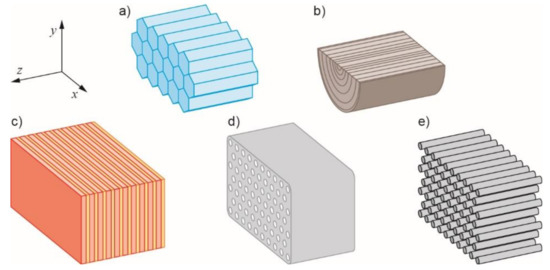
Figure 2.
Some examples of uniaxially anisotropic media: (a) a hexagonal crystal, (b) wood, (c) a layered structure, (d) a honeycomb structure, (e) a woodpile structure.
First, we get Γ and P as a function of S11 and S21. The Rosetta Stone of understanding the problem is Figure 3, showing a network model of an air-filled rectangular waveguide with a MUT placed. Based on this model, a graph of signal flow was plotted. Based on the graph, the Mason’s rule formulas [25,26], used in the literature on the subject, are presented.
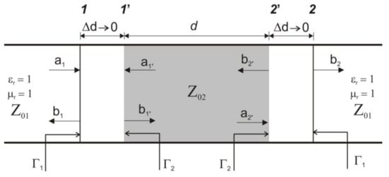
Figure 3.
Air-filled waveguide with the dielectric layers.
2.2. Determination of Γ and P as Functions of S11 and S21
The considered structure is shown in Figure 3. It is divided into five parts by four theoretical surfaces perpendicular to the waveguide’s propagation axis: 1, 1′, 2′, 2.
Air-filled parts of the waveguide have relative permittivity and permeability equal to 1, whereas layers of dielectric have their own specific values, and a specific complex propagation constant results from them. Respective impedances Z01 for air-filled, and Z02 for dielectric-filled waveguide can also be determined. The dielectric layer, 1′-2′, has length d, layers 1-1′ and 2-2′ have lengths tending to zero, the lengths of the outer layers are out of consideration. Additionally, incident Cs, ax, and reflected bx (x = {1, 1′, 2′, 2}) complex normalized wave-voltage amplitudes are marked for each connection surface. Last, there is no reflection from behind the 2 surface, nor from the 1 surface outside. This structure may be analyzed using a signal-flow graph approach.
Let us define the reflection coefficients at the interface between the layers as:
and the propagation factor P (transmittance through the dielectric layer) as:
where kz = β − jα is the complex wavenumber, and β and α are the phase and attenuations coefficient, respectively. Figure 4 shows a graph of the signal flow adequate to the analyzed structure.
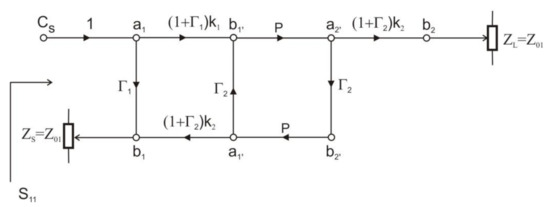
Figure 4.
Signal-flow graphs of the air-filled waveguide with the dielectric layers.
Based on this graph, the Mason rule [25,26] can be used to determine the transmittance Tax-bx between the ax and bx nodes.
where
T—source-to-sink transmittance of the graph;
Ti—the ith forward-path transmittance between the initial and out nodes;
Lk(j)—the kth loop transmittance; j—of this kind, occurring in the graph;
Lk,i(j)—the kth loop transmittance not touching the ith path.
The transmittance between nodes a1 and b1 is the scattering matrix coefficient S11
where k1 = 1/μz, k2 = μz for TE modes, or k1 = 1/εz, k2 = εz for TM modes; moreover, Γ1 = −Γ2.
Taking this into account, and introducing the designation Γ = Γ1, we get:
In the same way, the formula for S21, which is the transmittance between nodes CS and b2, can be derived:
The scattering-matrix elements S11 and S21 are expressed by the electric field reflection coefficient Γ and the propagation factor P, in the same form as for the isotropic medium. The system of Equations (6) and (8) will remain unchanged if Γ is mutually replaced with P, and S21 with S11. Moreover, the sum and difference of S21 and S11 can be expressed in a simple form:
By eliminating P or Γ from the above equations, quadratic equations can be obtained:
where
The solutions to the above equations are:
or
At this point, it is worth noting the ambiguity of the resulting pair of non-trivial solutions (Γ, P). Firstly, a quadratic equation has two solutions. Secondly, in the domain of complex numbers, the root in expressions (12) and (13) has two values.
This ambiguity is usually removed by adopting the solution for which |Γ| ≤ 1. It is true for the passive medium. Once Γ is determined, P is found as (cf. e.g., refs. [3,8]):
The pairs (Γ, P) can be expressed in terms of the material parameters of the medium, and have a different form depending on the considered waveguide mode. The method is based on the use of two pairs of solutions, (ΓTE, PTE) and (ΓTM, PTM), determined in terms S11 and S21 for TE and TM polarization, respectively. This enables their direct application for the extraction of complex components of permittivity and permeability tensors.
For technical reasons, the frequency fTE(TM) used for the TE10 and TM11 modes may be different. For instance, k0TE(TM) and λ0TE(TM) are wavenumbers and wavelengths in a vacuum, respectively.
where c is the velocity of light in a vacuum. Let us introduce the relative sample thickness dTE(TM), and the transverse dimensions of the waveguide aTE(TM) and bTE(TM):
Next, let us define the dimensionless relative wavenumbers KzTE(TM), and the relative cut-off wavenumbers KTE(TM)
where k10 and k11 are the cut-off wavenumbers for the TE10 and TM11 modes, respectively.
The propagation factors PTE(TM) can be rewritten as
where . Then
where nTE(TM) are the branch cut numbers of a complex logarithm.
A relative wave impedance zTE(TM) (the ratio of the wave impedance in the medium, to the wave impedance in an air-filled waveguide) can be expressed in terms of the electric field reflection coefficient ΓTE,TM, by the formula
Next, we will show how to obtain the complex material parameters εx, εy, εz, μx, μy, and μz using algebraic transformations.
2.3. Extraction of Material Parameters Using z and Kz—Configuration A
For transversely isotropic configuration, Equations (21) and (22) have the form
We have obtained a system of four Equations (23)–(26), from which the complex material parameters εx, εz, μx, and μz should be determined. Equations (23) and (24) can be rewritten as:
Multiplying the above expressions side by side, we get μx
Similarly, from (25) and (26), we obtain εx
Using (24) and (26) the remaining parameters, μz and εz can be expressed by μx and εx
Equation (32) shows that the TM11 mode is necessary to determine the parameter εz. However, in the case of this mode and a non-magnetic medium (μx = μy = μz = 1), it is enough to use (30) and (32) to uniquely determine εx and εz. This is not possible using the TE10 mode.
To extract parameters εr and μr of an isotropic MUT (εx = εy = εz = εr, μx = μy = μz = μr), we can use the results (28) and (31) for the TE10 mode (see, e.g., ref. [3])
or (30) and (32) for the TM11 mode
None among (28), (30), (31), and (32) for uniaxial anisotropy, or (35) and (36) for isotropy, has yet been reported in the scientific literature.
2.4. Extraction of Material Parameters Using z and Kz—Configuration B
In the case of the configuration B, only the TE10 mode can be considered. For the most general biaxial medium, Equations (21) and (22) have the form:
By writing (37) and (38) as
the parameter μx can be obtained
Then, for non-magnetic media, using (38) can determin εy
Since the TM11 mode is disabled for biaxial anisotropy, this can be a simple test of its existence or non-existence.
3. Simulations and Measurements
3.1. Description of the Configuration
Measurements in a rectangular waveguide, especially using the TE10 and TM11 modes, have some known advantages over the use of the TEM mode in a coaxial line, or TEM waves in an open microwave path:
- the isolation of signals from the external environment in a closed microwave path, and the possibility of using a smaller sample and its more precise positioning, compared to the so-called free-space methods; and
- the easier preparation of the sample in the form of a hexahedron, than of a cylinder in a coaxial line.
For the experiments, one rectangular waveguide with dimensions a = 40 mm, b = 20 mm, and two C-W adapters, were used to excite the TE10 and TM11 modes in the waveguide. Measurements were made at 6 GHz and 10.55 GHz for the TE10 and TM11 modes, respectively. A C-W adapter with a magnetic loop was used to excite the TE10 mode. To excite the TM11 mode, a C-W adapter with electrical coupling in the form of an antenna was designed and manufactured.
The proposed measurement system is shown in Figure 5.
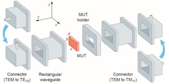
Figure 5.
The proposed measurement system.
3.2. TM Mode Coax-to-Waveguide Adapter Design
Using the CST Studio Suite® program, the C-W adapter was modeled for a rectangular waveguide in the 10–11 GHz band. The adapter matches the Z0 = 50 Ω TEM coax line impedance to the wave impedance of the TM11 mode, and ensures the excitation of this mode. Simulations of such a model were carried out. The simulation results are shown in Figure 6, Figure 7 and Figure 8.
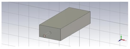
Figure 6.
A simulation structure containing a rectangular waveguide, together with a C-W adapter.
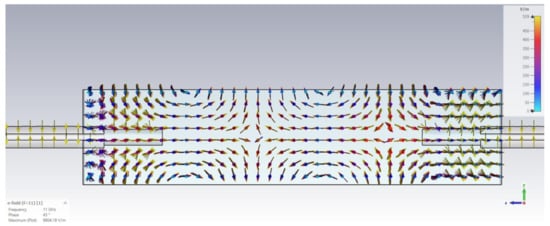
Figure 7.
Cross-section of the distribution of the electric field vector E in the rectangular waveguide.
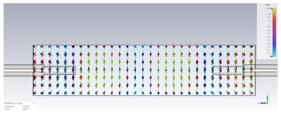
Figure 8.
Cross-section of the distribution of the magnetic field vector H in the rectangular waveguide.
The simulation results presented in Figure 7 and Figure 8 confirm the excitation of the TM11 mode in the rectangular waveguide. The electric field E has the component along the direction of wave propagation. On the other hand, the magnetic field H, at any point in the waveguide space, is transverse to the direction of wave propagation. To ensure the excitation of the TM11 mode with the longitudinal component of the electric field vector, a radiator located in the middle of the front and rear walls of the waveguide was used, as shown in Figure 6 and Figure 9. Figure 10 shows the result of the simulation of the waveguide-scattering matrix coefficients.
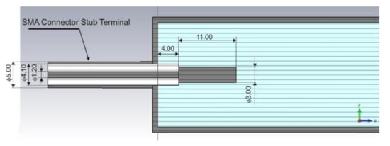
Figure 9.
Dimensions (in mm) of the C-W adapter for the waveguide-supporting the TM11 mode.
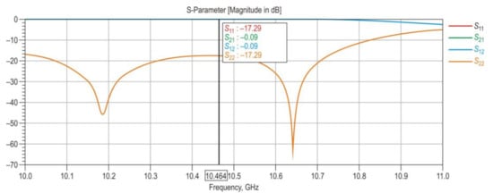
Figure 10.
Simulation results of the scattering parameters S11 and S21 in an empty waveguide with the TM11 mode.
3.3. Practical Implementation
Figure 11 shows a view of the C-W adapter, designed according to the project.
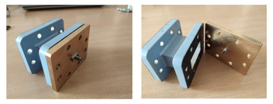
Figure 11.
TM11 mode C-W adapter.
A view of the waveguide structure is shown in Figure 12. This figure also shows the result of the measurements of the parameters S11 and S21 of the waveguide structure with the excited TM11 mode. The measurements S11 and S21 fully confirmed the simulation results of the TM11 mode C-W adapter.
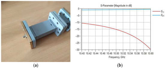
Figure 12.
An empty waveguide supporting the TM mode, (a) measured S-parameters dB[S11] (red), (b) dB[S21]] (blue).
3.4. Measurement Results
Measurements were made at two frequencies: fTE = 6 GHz for TE10 mode, and fTM = 10.55 GHz for the TM11 mode. In both cases, during the measurements, the tested material sample was in a rectangular waveguide, in which the type of C-W adapters was successively changed, depending on the analyzed mode. The measurements of the parameters S11 and S21 of the waveguide structure with the sample placed in it were carried out using a vector network analyzer (VNA). This is the most effective technique for measuring S-parameters. Using this instrument allowed us to measure S-parameters with high accuracy in relation to previously calibrated measurement gates. Measurements were made with a P9373B Streamline Vector Network Analyzer, 9 kHz to 14 GHz, 2-port. The VNA calibration was performed using the N7553A Electronic Calibration Module (ECal), DC-14 GHz, 2-port module that supports 3.5 mm 50 Ω connectors.
To reduce measurement errors, the procedure described in application note [27] was used. This application note described the techniques of de-embedding S-parameter networks with a device under test. Using the error-correcting algorithms of the vector network analyzer, the error coefficients can be modified, so that the process of de-embedding two port networks can be performed directly on the analyser in real time. This allowed us to use the de-embedding process, resulting in very accurate measurements.
Several isotropic and non-magnetic materials, whose electromagnetic parameters are described in the scientific literature, were selected for the measurements. The following materials were tested: PA-6 (Polyamide 6), FR4 (Epoxy Fiberglass Laminate), PVDF (Polyvinylidene Fluoride), and PTFE (Polytetrafluoroethylene).
The properties of the materials confirmed in the literature are presented in Table 1.

Table 1.
Properties of tested materials found in literature.
Table 2 and Table 3 shows the measurements of the S11 and S21, and calculation results of relative permittivity εr = ε′ − jε″ and relative permeability μr = μ′ − jμ″ for the TM11 and TE10 modes, respectively.
Table 2.
Measurements and calculation results for the TM11 mode (fTM = 10.55 GHz).
Table 3.
Measurements and calculation results for the TE10 mode (fTE = 6 GHz).
Measurements of the PA-6 sample for the TE10 and TM11 modes gave a consistent result of relative permittivity ε′ = 3.23. Similar values of parameters of this material are presented in [28]. For the remaining materials, there is an analogous agreement between the measurement results obtained using the TE10 and TM11 modes. For the FR4 sample, the obtained values were confirmed in [29,30], for the PVDF in [31,36], and for the PTFE in [5,32,33,34,35].
4. Discussion
The comparison of measurements presented in Table 2 (the novel method) and Table 3 (the traditional method) confirms the validity of using the TM11 mode to extract the material parameters μr and εr of the isotropic medium.
The proposed method of extracting material parameters using the TM11 mode has several advantages over the traditional method using the TE10 mode.
- The first is due to the permittivity εr extraction resulting from (35). The traditional method requires first the determination of permeability μr, from (33), and then εr, from (34). The proposed method does not require the prior determination of permeability, so it does not introduce an additional error. In broadband studies, a known disadvantage of the NRW method is instability at frequencies corresponding to integer multiples of one-half wavelength in the MUT. An effective and widely used method of eliminating these instabilities is the iterative method, first described in [5]. This method applies to non-magnetic materials, i.e., with μr = 1. Using the TM11 mode does not require this assumption.
- When the medium is non-magnetic (which is a common case) and uniaxial, both relative permittivity εx, and εz can be determined using the TM11 mode without changing the position of the sample. This cannot be done with the TE11 mode, because the latter does not has an electric field z-component.
- In turn, the use of the TM11 and TE10 modes allows us to determine all four parameters of the uniaxial medium, without changing the position of the sample.
An experimental confirmation of the presented theoretical results for uniaxial anisotropic materials will be the direction of further research.
The work fits into the broader context of verifying the properties of materials using various methods of microwave measurements [37,38]. In a narrower context, it provides an alternative to using TEM or the TE10 modes in transmission/reflection measurement techniques.
At this point, it is necessary to mention the work [39], where the method of extracting the parameters of biaxial media in the rectangular waveguide, using the TM11 mode, is presented. We questioned the theoretical basis of this work in comments [40] accepted for publication. Quite simply, the TM11 mode is not propagated in the biaxial medium, as we have stated in [24], and clearly indicated in this paper.
Author Contributions
Conceptualization, A.D. and W.S.; methodology, A.D.; validation, W.S., P.P. and A.D.; formal analysis, W.S. and A.D.; investigation, P.P.; data curation, P.P.; writing—original draft preparation, A.D.; writing—review and editing, W.S. and A.D.; visualization, A.D. and W.S.; supervision, W.S. All authors have read and agreed to the published version of the manuscript.
Funding
This work was financed by Military University of Technology under Research Project UGB 868.
Data Availability Statement
Not applicable.
Conflicts of Interest
The authors declare no conflict of interest.
References
- Nicolson, A.M.; Ross, G.F. Measurement of the intrinsic properties of materials by time-domain techniques. IEEE Trans. Instrum. Meas. 1970, 19, 377–382. [Google Scholar] [CrossRef]
- Weir, W.B. Automatic measurement of complex dielectric constant and permeability at microwave frequencies. IEEE 1974, 62, 33–36. [Google Scholar] [CrossRef]
- Rothwell, E.J.; Frasch, J.L.; Ellison, S.M.; Chahal, P.; Ouedraogo, R.O. Analysis of the Nicolson-Ross-Weir Method for Characterizing the Electromagnetic Properties of Engineered Materials. Prog. Electromagn. Res. 2016, 157, 31–47. [Google Scholar] [CrossRef]
- Costa, F.; Borgese, M.; Degiorgi, M.; Monorchio, A. Electromagnetic Characterisation of Materials by Using Transmission/Reflection (T/R) Devices. Electronics 2017, 6, 95. [Google Scholar] [CrossRef]
- Baker-Jarvis, J.; Vanzura, E.J.; Kissick, W.A. Improved technique for determining complex permittivity with the transmission/reflection method. IEEE Trans. Microw. Theory Tech. 1990, 38, 1096–1103. [Google Scholar] [CrossRef]
- Smith, D.R.; Schultz, S.; Markoš, P.; Soukoulis, C.M. Determination of effective permittivity and permeability of metamaterials from reflection and transmission coefficients. Phys. Rev. B 2002, 65, 195104. [Google Scholar] [CrossRef]
- Markos, P.; Soukoulis, C.M. Transmission properties and effective electromagnetic parameters of double negative metamaterials. Opt. Express 2003, 11, 649–661. [Google Scholar] [CrossRef]
- Varadan, V.V.; Ro, R. Unique Retrieval of Complex Permittivity and Permeability of Dispersive Materials from Reflection and Transmitted Fields by Enforcing Causality. IEEE Trans. Microw. Theory Tech. 2007, 55, 2224–2230. [Google Scholar] [CrossRef]
- Chen, X.; Grzegorczyk, T.M.; Wu, B.-I.; Pacheco, J.; Kong, J.A. Robust method to retrieve the constitutive effective parameters of metamaterials. Phys. Rev. E 2004, 70, 016608. [Google Scholar] [CrossRef]
- Barroso, J.J.; de Paula, A.L. Retrieval of Permittivity and Permeability of Homogeneous Materials from Scattering Parameters. J. Electromagn. Waves Appl. 2010, 24, 1563–1574. [Google Scholar] [CrossRef]
- de Paula, A.L.; Rezende, M.C.; Barroso, J.J. Modified Nicolson-Ross-Weir (NRW) method to retrieve the constitutive parameters of low-loss materials. In Proceedings of the SBMO/IEEE MTT-S International Microwave and Optoelectronics Conference (IMOC 2011), Natal, Brazil, 29 October–1 November 2011; pp. 488–492. [Google Scholar] [CrossRef]
- Arslanagić, S.; Hansen, T.V.; Mortensen, N.A.; Gregersen, A.H.; Sigmund, O.; Ziolkowski, R.W.; Breinbjerg, O. A Review of the Scattering-Parameter Extraction Method with Clarification of Ambiguity Issues in Relation to Metamaterial Homogenization. IEEE Antennas Propag. Mag. 2013, 55, 91–106. [Google Scholar] [CrossRef]
- Angiulli, G.; Versaci, M. Retrieving the Effective Parameters of an Electromagnetic Metamaterial Using the Nicolson-Ross-Weir Method: An Analytic Continuation Problem Along the Path Determined by Scattering Parameters. IEEE Access 2021, 9, 77511–77525. [Google Scholar] [CrossRef]
- Chen, H.; Zhang, J.; Wang, Y.; Che, W.; Huang, Z.; Qiao, Y.; Luo, J.; Xue, Q. An Improved NRW Method for Thin Material Characterization Using Dielectric Filled Waveguide and Numerical Compensation. IEEE Trans. Instrum. Meas. 2022, 71, 1–9, Art no. 8003009. [Google Scholar] [CrossRef]
- Damaskos, N.J.; Mack, R.B.; Maffett, A.L.; Parmon, W.; Uslenghi, P.L.E. The inverse problem for biaxial materials. IEEE Trans. Microw. Theory Tech. 1984, 32, 400–405, Erratum in IEEE Trans. Microw. Theory Tech. 1992, 40, 174. [Google Scholar] [CrossRef]
- Akhtar, M.J.; Feher, L.E.; Thumm, M. A waveguide-based two-step approach for measuring complex permittivity tensor of uniaxial composite materials. IEEE Trans. Microw. Theory Tech. 2006, 54, 2011–2022. [Google Scholar] [CrossRef]
- Chen, H.; Zhang, J.; Bai, Y.; Luo, Y.; Ran, L.; Jiang, Q.; Kong, J.A. Experimental retrieval of the effective parameters of metamaterials based on a waveguide method. Opt. Express 2006, 14, 12944–12949. [Google Scholar] [CrossRef]
- Ishizaki, T.; Kida, S.; Awai, I. A measurement method of material parameters for uniaxially anisotropic artificial dielectrics. IEICE Electron. Express 2010, 7, 810–816. [Google Scholar] [CrossRef]
- Xu, X. Double waveguide method to retrieve the electromagnetic parameters of biaxial anisotropic materials. Electron. Lett. 2018, 54, 5436. [Google Scholar] [CrossRef]
- Hasar, U.C.; Buldu, G.; Bute, M.; Muratoglu, A. Calibration-free extraction of constitutive parameters of magnetically coupled anisotropic metamaterials using waveguide measurements. Rev. Sci. Instrum. 2017, 88, 104702. [Google Scholar] [CrossRef]
- Hasar, U.C.; Buldu, G.; Barroso, J.J. Waveguide Method for Electromagnetic Parameter Extraction of Weakly Coupled Metamaterials. IEEE Microw. Wirel. Compon. Lett. 2017, 27, 851–853. [Google Scholar] [CrossRef]
- Jiang, Z.; Bossard, J.A.; Wang, X.; Werner, D.H. Synthesizing metamaterials with angularly independent effective medium properties based on an anisotropic parameter retrieval technique coupled with a genetic algorithm. J. Appl. Phys. 2011, 109, 013515. [Google Scholar] [CrossRef]
- Castanié, A.; Mercier, J.-F.; Félix, S.; Maurel, A. Generalized method for retrieving effective parameters of anisotropic metamaterials. Opt. Express 2014, 22, 29937–29953. [Google Scholar] [CrossRef] [PubMed]
- Dukata, A.; Susek, W. Transmission Parameters of an Anisotropic Layered Structure in the Waveguide. In Proceedings of the SPIE 11442, Radioelectronic Systems Conference, Jachranka, Poland, 20–21 November 2019. [Google Scholar] [CrossRef]
- Mason, S.J. Feedback Theory–Some Properties of Signal Flow Graphs. Proc. IRE 1953, 41, 1144–1156. [Google Scholar] [CrossRef]
- Mason, S.J. Feedback Theory–Further Properties of Signal Flow Graphs. Proc. IRE 1956, 44, 920–926. [Google Scholar] [CrossRef]
- Application Note 1364-1, Agilent De-Embedding and Embedding S-Parameter Networks Using a Vector Network Analyzer; Agilent Technologies, Inc.: Santa Clara, CA, USA, 2004.
- Pittella, E.; Piuzzi, E.; Russo, P.; Fabbrocino, F. Microwave Characterization and Modelling of PA6/GNPs Composites. Math. Comput. Appl. 2022, 27, 41. [Google Scholar] [CrossRef]
- Guo, Z.; Pan, G.; Hall, S.; Pan, C. Broadband Characterization of Complex Permittivity for Low-Loss Dielectrics: Circular PC Board Disk Approach. IEEE Trans. Antennas Propag. 2009, 57, 3126–3135. [Google Scholar] [CrossRef]
- Narayanan, P.M. Microstrip Transmission Line Method for Broadband Permittivity Measurement of Dielectric Substrates. IEEE Trans. Microw. Theory Tech. 2014, 62, 2784–2790. [Google Scholar] [CrossRef]
- Indrusiak, T.; Pereira, I.M.; Pontes, K.; Pereira, E.C.; Peixoto, G.G.; Migliano, A.C.; Soares, B.G. Hybrid carbonaceous materials for radar absorbing poly (vinylidene fluoride) composites with multilayered structures. SPE Polym. 2021, 2, 62–73. [Google Scholar] [CrossRef]
- Chen, Y.C.; Lin, H.C.; Lee, Y.D. The effects of filler content and size on the properties of PTFE/SiO2 composites. J. Polym. Res. 2003, 10, 247–258. [Google Scholar] [CrossRef]
- Yakubu, A.; Abbas, Z.; Ibrahim, N.A.; Fahad, A. The effect of ZNO nanoparticles filler on complex permittivity of ZNO-PCL nanocomposite at microwave frequency. Phys. Sci. Int. J. 2015, 6, 196–202. [Google Scholar] [CrossRef]
- Wu, C.; Liu, Y.; Lu, S.; Gruszczynski, S.; Yashchyshyn, Y. Convenient waveguide technique for determining permittivity and permeability of materials. IEEE Trans. Microw. Theory Tech. 2020, 68, 4905–4912. [Google Scholar] [CrossRef]
- Yashchyshyn, Y.; Derzakowski, K.; Wu, C.; Cywiński, G. W-band sensor for complex permittivity measurements of rod shaped samples. IEEE Access 2021, 9, 111125–111131. [Google Scholar] [CrossRef]
- Meng, X.M.; Zhang, X.J.; Lu, C.; Pan, Y.F.; Wang, G.S. Enhanced absorbing properties of three-phase composites based on a thermoplastic-ceramic matrix (BaTiO3+ PVDF) and carbon black nanoparticles. J. Mater. Chem. A 2014, 2, 18725–18730. [Google Scholar] [CrossRef]
- Krupka, J. Frequency domain complex permittivity measurements at microwave frequencies. Meas. Sci. Technol. 2006, 17, R55–R70. [Google Scholar] [CrossRef]
- Krupka, J. Microwave Measurements of Electromagnetic Properties of Materials. Materials 2021, 14, 5097. [Google Scholar] [CrossRef]
- Kiani, M.; Abdolali, A.; Tayarani, M. Rectangular Waveguide Characterization of Biaxial Material Using TM11 Mode. IEEE Trans. Instrum. Meas. 2022, 71, 8005615. [Google Scholar] [CrossRef]
- Dukata, A.; Susek, W. Comments on “Rectangular Waveguide Characterization of Biaxial Material Using TM11 Mode”. IEEE Trans. Instrum. Meas 2023. accepted for publication. [Google Scholar]


Disclaimer/Publisher’s Note: The statements, opinions and data contained in all publications are solely those of the individual author(s) and contributor(s) and not of MDPI and/or the editor(s). MDPI and/or the editor(s) disclaim responsibility for any injury to people or property resulting from any ideas, methods, instructions or products referred to in the content. |
© 2023 by the authors. Licensee MDPI, Basel, Switzerland. This article is an open access article distributed under the terms and conditions of the Creative Commons Attribution (CC BY) license (https://creativecommons.org/licenses/by/4.0/).