This section introduces the design and implementation of our EinStein würfelt nicht program, Monte_Alpha. We will elaborate on three aspects: the representation of the game board, the search algorithm, and the design of the die roll. The following sections will explain each of these three parts in detail.
4.1. Bitboard Representation
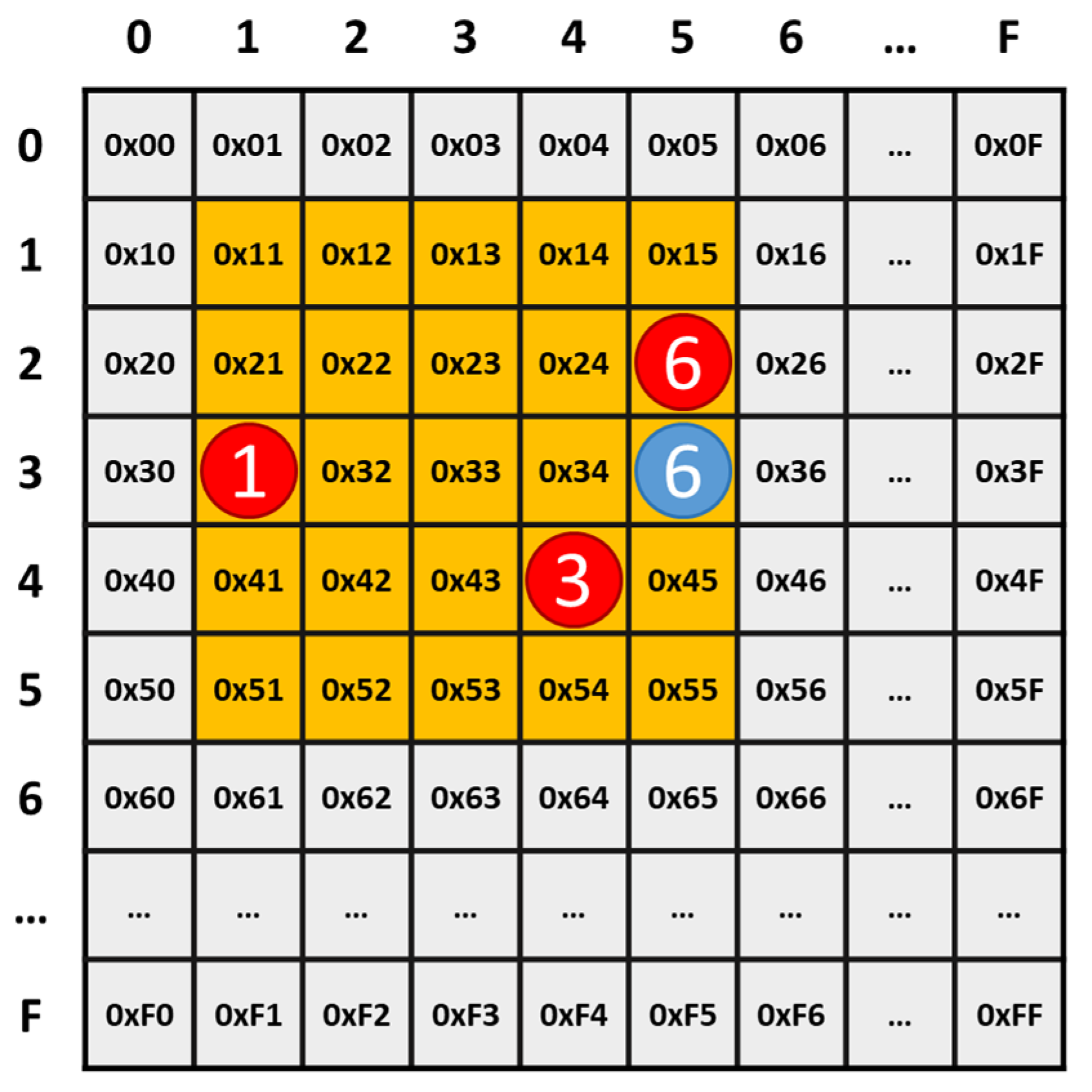
Monte_Alpha uses a one-dimensional array data structure to record the state of the board. In order to make the program execution more efficient, many bitwise operations are used in the development of the program. Therefore, the board representation is also presented in hexadecimal format. The Board (which comprises 256 spaces (16
16 elements)) is used to record the state of the board and is as shown in
Figure 3. Herein, the value of the board position, Board [position], ranges from −1 to 12, where −1 denotes that this position is outside of the range of the game board, 0 indicates that there is no piece in this position, 1 to 6 represent the blue pieces numbered 1 to 6, respectively, and 7 to 12 represent the red pieces numbered 1 to 6, respectively.
Additionally, the used fields are the 25 squares in the orange area (0x11~0x55) in
Figure 3. Although this design scheme wastes a large amount of storage space and is not as efficient as the pure bitboard scheme [
35,
36], it has the following advantages:
Fast move generation: Taking
Figure 3 as an example, the red piece with the number 3 (0x44) can move to the right (0x45), down (0x54), or diagonally down to the right (0x55). The move can be generated quickly by adding an increment (INC). The operation is as follows:
where INC = {0x01, 0x10, 0x11}.
Fast validation of move legality: The performance of the bitboard is much faster than using a two-dimensional array data structure [
37]. It can be quickly determined whether the movement of a piece is within the valid range of the board. Continuing the example in
Figure 3, suppose the right move (0x45) for the red piece with number 3 is expanded. The validation operation is as follows:
Since there is no piece in position 0x45,
= 0 and the value of Formula (3) is true, which means the right move (0x45) for the red piece with the number 3 is legal. In another example, suppose the diagonally down move (0x36) for the red piece with the number 6 is expanded. The validation operation is as follows:
Since the position 0x36 is outside of the range of the game board, as shown in the gray area in
Figure 3, Board [0x36] = −1 and the value of Formula (4) is false, which means the diagonally down move (0x36) for the red piece with number 6 is illegal.
Quick access to board coordinates: Continuing the example in
Figure 3, suppose the right move (0x45) is selected. The board coordinates can be obtained quickly through the following bitwise operations:
where its corresponding coordinates are the fourth row (high-order hexadecimal digit) and the fifth column (low-order hexadecimal digit).
Convenient for developers to debug: Using a two-dimensional array or tuple has the advantage of high readability while using a bitboard has the advantage of better performance. Although the overall execution performance is a little lower than when using a pure bitboard, the representation of our bitboard is as simple and clear as using a two-dimensional array.
4.2. Search Algorithm
Due to the probabilistic nature of the die-rolling phase in Einstein würfelt nicht, using the Monte Carlo method represents a good option. Therefore, the search algorithm of Monte_Alpha adopts the Upper Confidence bounds applied to Trees (UCT) algorithm introduced in
Section 2, which uses the UCB’ formula in Monte Carlo Tree Search (MCTS). Because of the die-rolling steps involved in Einstein würfelt nicht, the expansion of the game tree becomes more complex. As a result, the original UCT cannot be directly applied to Einstein würfelt nicht.
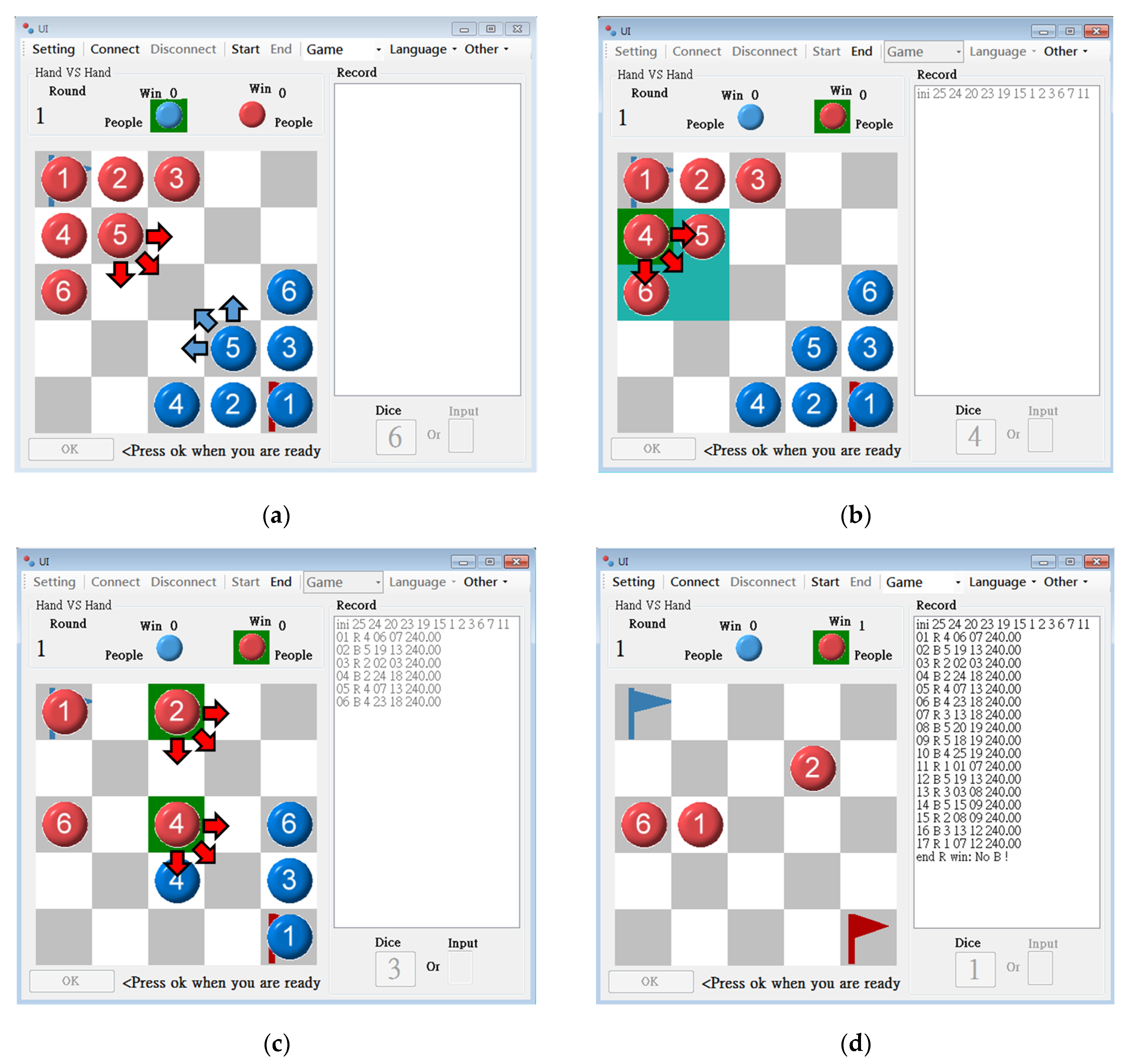
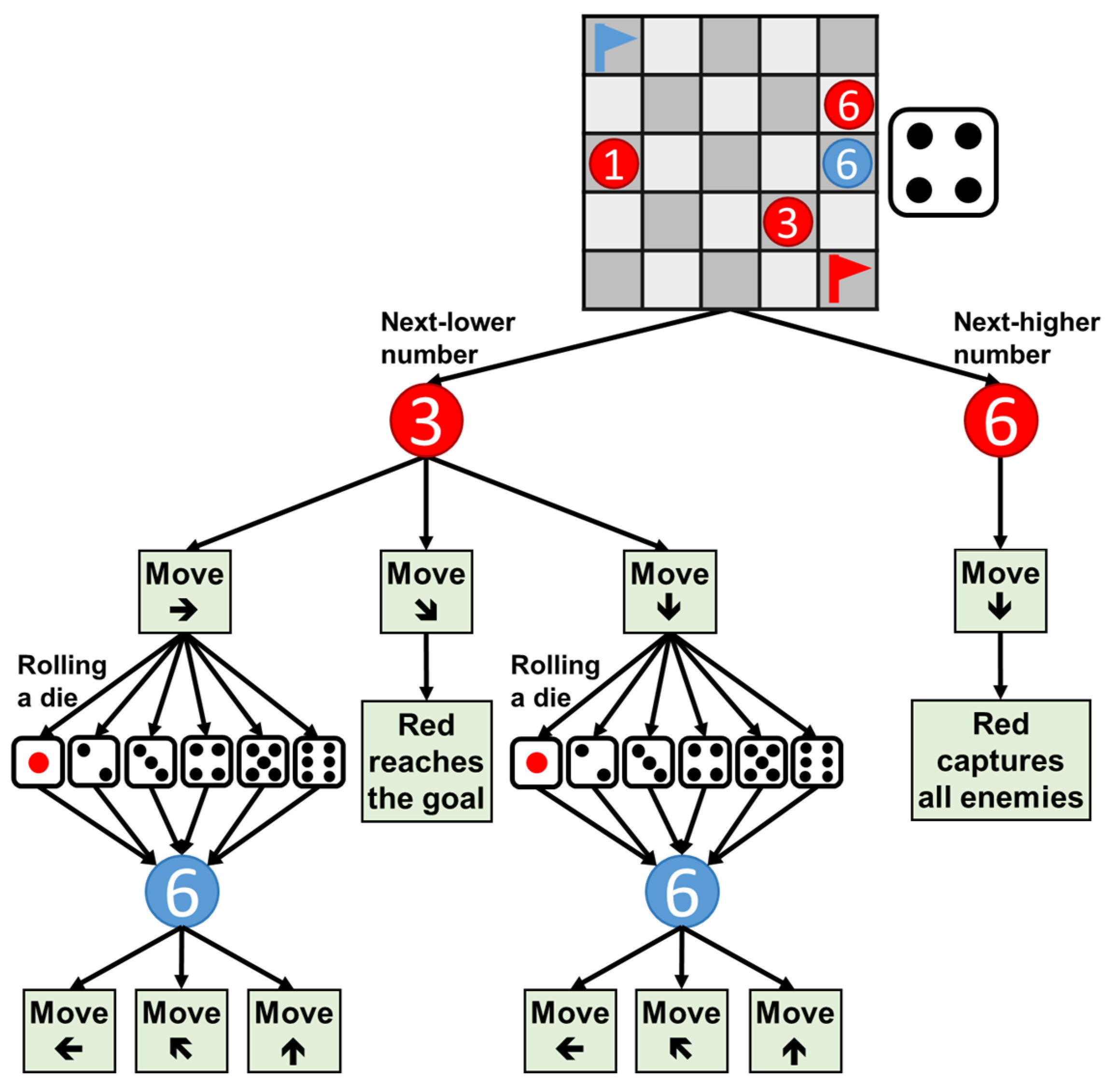
Figure 4 illustrates the search algorithm architecture of Monte_Alpha. The root node is special because its board state includes the number of points rolled on the die, determining which pieces (two pieces at most) can be moved, and each piece has at most three possible moves. In the example in
Figure 4, the given board comes with a die roll of 4, but red piece number 4 is no longer on the board. Therefore, the red player can choose either piece number 3 or 6, where red piece number 3 has three possible moves, and red piece number 6 can only move downward to capture blue piece number 6.
Furthermore, the nodes expanded below the root node are different from the root node. The expansion process requires simulating the rolling of the die to determine which pieces can be moved. Therefore, all possible die rolls from one to six must be considered. In the example in
Figure 4, the only blue piece that remains on the board is piece number 6, so no matter what number the die rolls, the blue player can only move piece number 6. In addition, the expansion process of the game tree follows the four steps of UCT. Finally, the move with the highest number of simulations is selected as the best decision for the given game state.
4.3. Design of Die Rolling
When designing the die-rolling action, the most intuitive method would be to first randomly generate a number between one and six and then check whether the piece with this number is still on the board. If the piece with this number is no longer on the board, the program would then look to both the left and right to find the piece with the closest number that is still on the board. For instance, as illustrated in
Figure 3, suppose the red player rolls a three, and the red piece labeled number 3 is still on the board. This is the best case and requires searching once. Alternatively, suppose the blue player rolls a one, and the blue piece labeled number 1 is no longer on the board. The program would then need to look to the right to find the adjacent piece that is still on the board, which is piece number 6. This is the worst case and requires searching six times. In general, if the rolled piece is no longer on the board, the program needs to search for the adjacent piece, which requires searching approximately three times on average, but the program also needs to check the pieces on the left and the right, so the overall number of searches is approximately six.
During implementation, Monte_Alpha uses bitwise operations, adding two variables to record the state of the blue and red pieces. For instance, with reference to
Figure 3, the binary value of the state of the blue pieces is as follows:
where the least significant bit represents piece number 1, and the most significant bit represents piece number 6. Similarly, the binary value of the red player’s pieces state is as follows:
To check whether the blue player still has pieces on the board, it is only necessary to determine whether blue_alive is not equal to zero. For example, in the right branch of
Figure 4, red piece number 6 will capture blue piece number 6. Afterward, blue_alive will become zero, indicating that the red player has captured all enemies and won the game. Similarly, the red player can also quickly determine whether there are still pieces in play using this command. Since there are only 2
6 combinations of a single player’s piece status, a probability distribution table can be pre-established for all piece combinations to speed up the program’s processing time.
In order to accelerate the efficiency of rolling the die, the probability of each die number appearing is converted into the number of times it appears and is stored in a probability table to speed up obtaining information about which pieces can be moved. Taking the red pieces in
Figure 3 as an example, the binary representation of the red piece status is 100101, which means that the pieces numbered 1, 3, and 6 are still on the board. The probabilities of those three pieces that can be moved are
(the probability of rolling a 1 is
, and there is a half chance of moving piece 1 when rolling a 2, with a probability of
),
(the probability of rolling a 3 is
, and there is a half chance of moving piece 3 when rolling a 2, 4 or 5, with a probability of
), and
(the probability of rolling a 6 is
, and there is a half chance of moving piece 6 when rolling 4 or 5, with a probability of
), respectively.
Position 100,101 in the probability table is a 10,000-element array with a value of one for elements 0 to 2499, a value of three for elements 2500 to 6666, and a value of six for elements 6667 to 9999. This indicates that when rolling the die 10,000 times, there are 2500 chances to move piece 1, 4167 chances to move piece 3, and 3333 chances to move piece 6. The contents of the array are as follows:
In this way, it only takes checking which pieces can be moved once by looking up the table. The operation is as follows:
During the process of game tree expansion, each simulation needs to go through a series of moves to reach the end state of the game. Assuming the depth of the simulation is , each simulation with Monte_Alpha only takes times, whereas the conventional method requires times. Therefore, as long as the number of simulations increases, the acceleration effect of Monte_Alpha is considerable, and this is where the advantage of Monte_Alpha lies.


