1. Introduction
Hyperspectral images (HSIs) are a particular type of remote sensing image with abundant spectral and spatial information [
1], which can be studied in many fields, including urban vegetation cover monitoring [
2], water detection [
3], agricultural resource detection [
4], and environmental protection [
5], etc. [
6,
7,
8]. Recently, HSI classification tasks have been the focus of HSI research [
9,
10]. However, the over-redundancy of spectral band information makes it hard to extract fine features, which has been a challenge for feature extraction. Traditional feature extraction methods, such as support vector machine (SVM) [
11,
12] and multinomial logistic regression (MLR) [
13,
14], have been developed to build pixel-wise-based classifiers for analyzing the HSI. Although enough spectral features can be extracted using these methods, the acquired classification maps are still noisy or blurry. To this end, denoising, deblurring, super-resolution, and feature fusion strategies were proposed to solve these issues. Recently, deep learning algorithms based on convolutional neural networks (CNNs) [
15] were found to have better performance in feature fusion [
16]. CNN can extract spatial information without destroying the original spatial structure [
17]. Specifically, deep learning algorithms have experienced a process from 1D-CNN [
18] and 2D-CNN [
19,
20,
21] to 3D-CNN [
22]. In comparison, 3D-CNN can extract spatial–spectral features by using 3D convolution, which makes full use of the 3D data information of the HSI compared with the 1D-CNN and 2D-CNN.
However, 3D-CNN suffers from overfitting and degradation. The residual network (ResNet) [
23] and the dense network (DenseNet) [
24] were proposed to solve these problems. For example, Zhong et al. [
25] proposed a spectral–spatial residual network (SSRN). They designed a consequent spatial–spectral residual block to sequentially learn the HSI’s discriminative features, effectively improving the classification accuracy. The disadvantage, however, is an exorbitantly long training time. Inspired by SSRN, Wang et al. [
26] designed a consequent spatial–spectral dense block based on DenseNet to improve feature reuse, which also helped to achieve better performance while reducing training time. To combine the advantages of the dense network and the residual network, Tu et al. [
27] proposed a residual dense and dilated convolution network (RDDC-3DCNN) with both residual and dense blocks to fuse the features hierarchically, and the accuracy was further improved. When facing the small sample issue, unsupervised and semi-supervised networks were proposed, such as the Conv–Deconv network [
28], generative adversarial networks (GANs) [
29], graph convolutional networks (GCNs) [
30], and robust self-ensembling network (RSEN) [
31], etc. These networks effectively improve the accuracy of HSI classification tasks.
The above studies show that networks with residual or dense structures can realize feature fusion from layer to layer and, thus, obtain finer features. But, as convolutional layers increase, most fine features tend to be reduced or even lost. To solve these issues, a lot of advanced techniques, such as feature fusion and attention mechanisms, have been applied to HSI classification tasks. Zhang et al. [
32] proposed a multi-scale dense network (MSDN) with a dense network as the backbone. The feature maps from low scale, medium scale, and high scale were used for feature fusion; this method ensured accuracy while improving the convergence speed, but the network has a vast number of parameters as well as a long training time. In addition, in the procedure of extracting spatial–spectral features, they did not find clear semantics for these feature maps. In [
33], a novel multi-scale dense network (MSDN-SA) was proposed, and the spectral-wise attention mechanism was employed in the field of HSI classification for the first time.
Subsequently, attention mechanisms have been successfully practiced and developed in HSI classification over the years. Li et al. [
34] proposed a 3D-SE-DenseNet based on a Squeeze-and-Excitation network (SENet) [
35], which enhanced the ability to extract spectral features by automatically learning to construct an SENet after each dense block. In [
17], a double-branch multi-attention network (DBMA) with the convolutional block attention module (CBAM) [
36] was proposed, which will significantly reduce the interference between two different kinds of features. Based on DBMA and the adaptive self-attention mechanism [
37], Li et al. [
38] proposed a double-branch dual-attention mechanism network (DBDA). The DBDA framework uses less training time while obtaining higher accuracy than DBAM. Qing et al. [
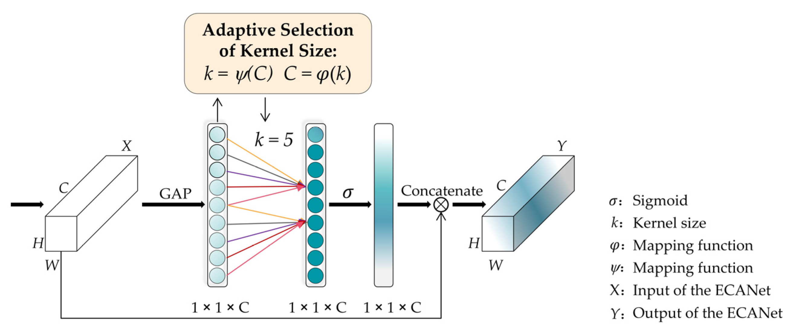
39] employed ECANet [
40] in their multi-scale residual convolutional neural network (MRA-Net) to fully exploit the core components obtained from the principal component analysis (PCA) [
41] technology, which successfully helped improve classification accuracy. Following that, Qing et al. [
42] again proposed a 3D self-attention [
43] multi-scale feature fusion network (3DSA-MFN), which can make full use of the contextual information of the HSI.
Very recently, the self-attention-based transformer [
44] has been widely used in HSI classification, which can better process sequential data. For example, the spatial–spectral transformer (SST) [
45] was proposed to solve the problem of gradient vanishing. In [
46], the SpectralTransformer was proposed to effectively process the sequence attributes of spectral features. In [
47], a spectral–spatial feature tokenization transformer (SSFTT) method was proposed to capture high-level semantic features. However, a transformer is relatively weak in discriminating local features [
48]. In addition, few of the networks above can better balance the convergence performance and classification accuracy, and these networks tend to have large loss fluctuations in the training process.
Therefore, in this paper, inspired by the advanced MSDN network and [
49], we propose an efficient channel attentional feature fusion dense network for HSI classification to better fuse features of inconsistent semantics and scales. To conclude, three major contributions have been made to this study:
We propose an efficient channel attentional feature fusion dense network (CA-FFDN) based on DenseNet and ECA. Our network has two main structures: feature extraction structure and feature enhancement structure. Principal component analysis (PCA) technology is applied to ensure the utilization of effective spectra and reduce noise interference.
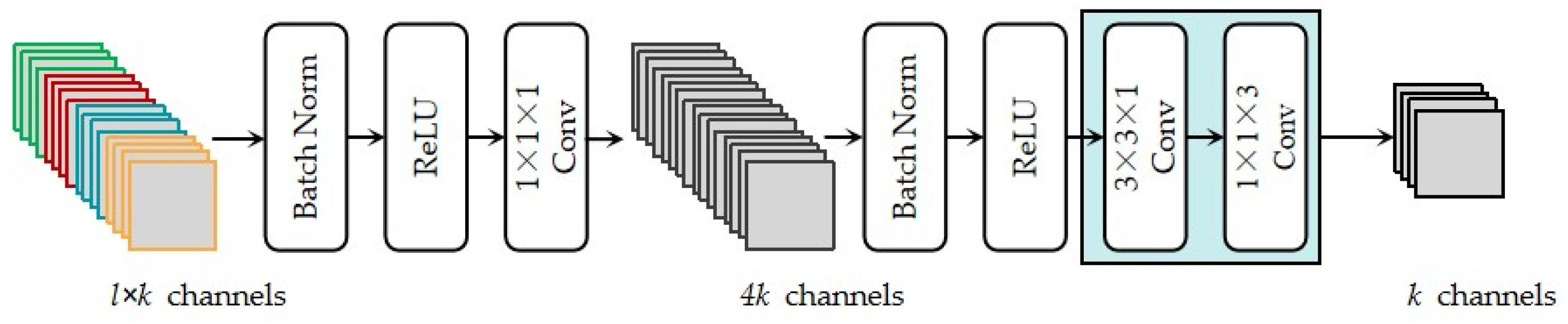
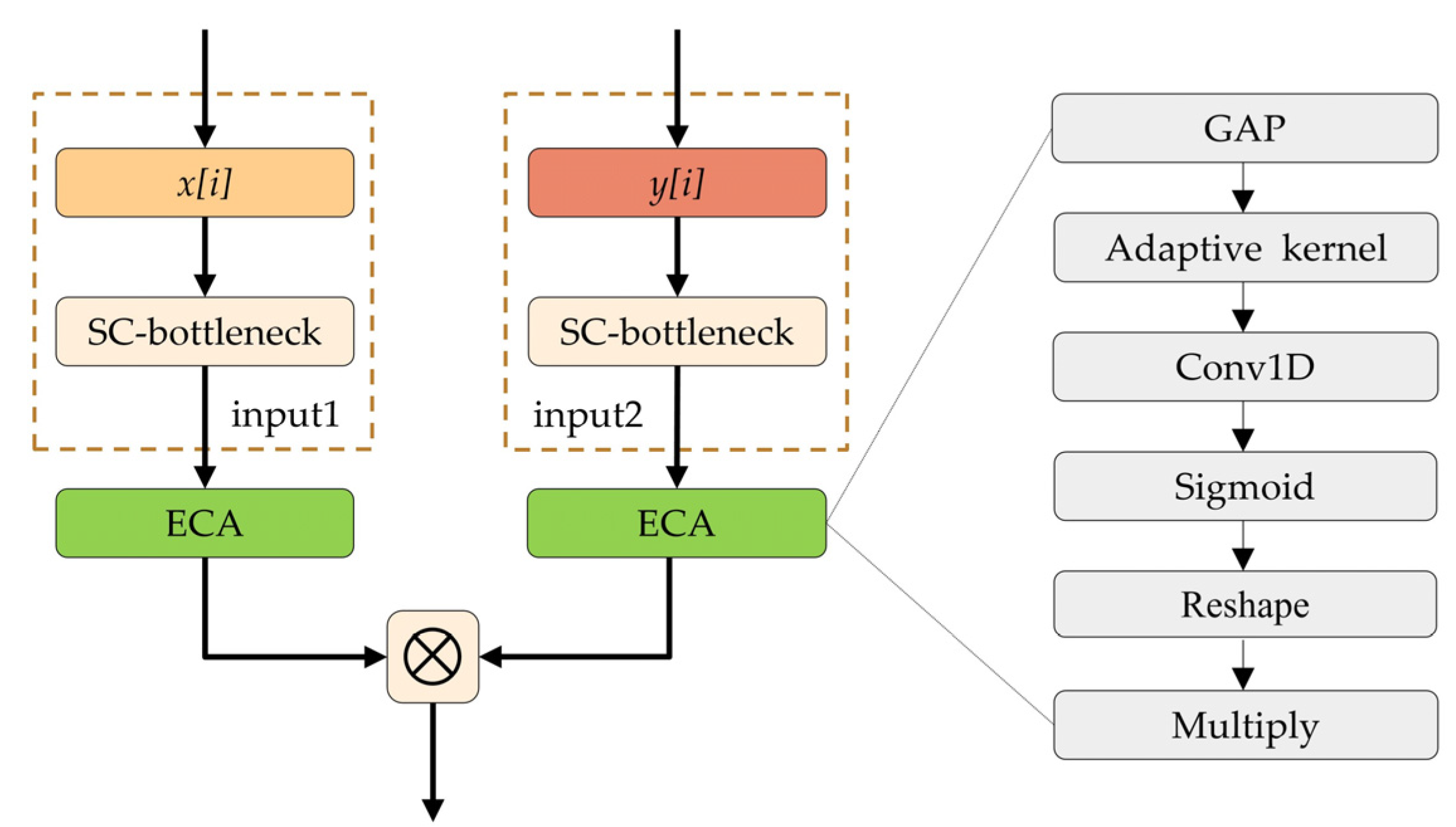
We employ the latest modified DenseNet as the backbone, which outstandingly reduces the parameter and training time in the network compared with MSDN. Meanwhile, an efficient attention mechanism is introduced to realize attentional feature fusion at two scales of the input and output layers, which suppresses the loss of spatial–spectral features and accelerates the convergence speed of the network.
The proposed network has state-of-the-art classification results in comparison experiments with five advanced networks under the same experimental environment on three open-source datasets.
The rest of the paper is organized as follows:
Section 2 introduces the proposed framework.
Section 3 details the experimental results and analysis. Finally,
Section 4 concludes the paper.
3. Experimental Results and Analysis
The hardware environment for all experiments utilizes an Intel(R) Core(TM) i7-9700K CPU @ 3.60 GHz processor with 64 GB of RAM and NVIDIA GeForce RTX 2080Ti GPU. The software environment is based on the deep learning framework of Tensorflow-gpu for Windows 10, utilizing the Pycharm2020 platform with Python 3.6 compiler.
3.1. Experimental Dataset
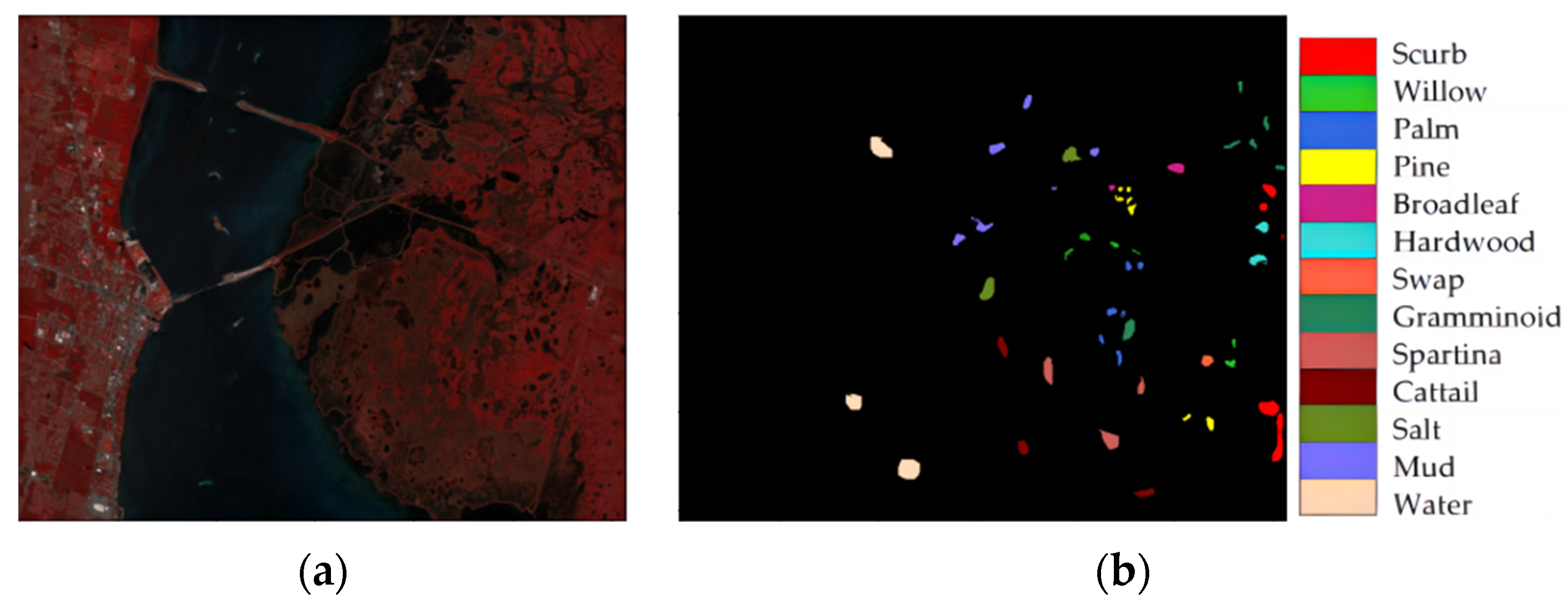
Three open-source hyperspectral datasets, Indian Pines (IP), Pavia of University (UP), and Kennedy Space Center (KSC) [
52], were selected as experimental subjects. We divided the datasets into the training set, validation set, and testing set after random shuffling, and it is worth mentioning that we followed [
34] to set the ratio of the samples. 20%:10%:70% for the IP and KSC datasets and 10%:10%:80% for the UP dataset. Last, but not least, overall accuracy (OA), average accuracy (AA), and kappa coefficient (K) are used for quantitative analysis of the experimental results. Higher metric values indicate that the network is more capable of classifying [
53].
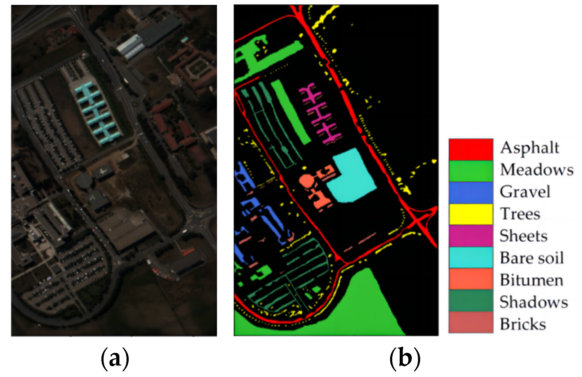
Table 1 shows the specific parameter settings of the datasets, and the false color maps of the IP, UP, and KSC datasets and their ground-truth maps are shown in
Figure 8,
Figure 9 and
Figure 10, respectively.
3.2. Experimental Setting
In our experiment, the batch size was set to 16, the RMSprop optimizer [
54] was selected to optimize the training loss, and the number of training iterations was set to 100, saving the best model for each iteration. We employed the grid search [
55,
56] method to choose the best learning rate, and the learning rate was set to 0.01, 0.001, 0.003, 0.0003, 0.0005, and 0.00005, respectively. The results showed that the optimal learning rate was 0.0003 on the three datasets.
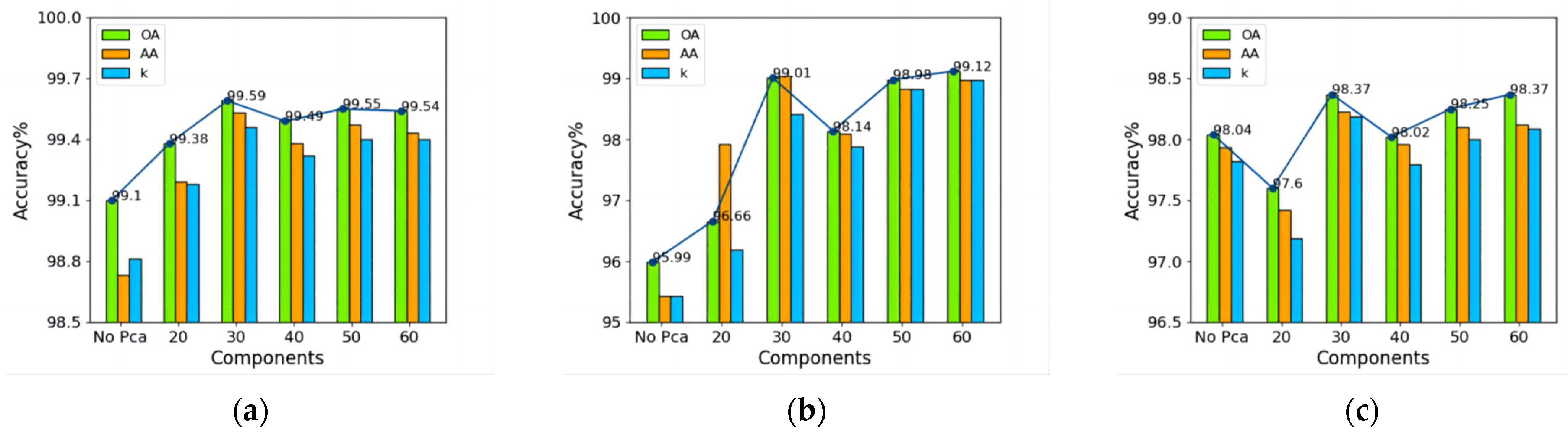
3.2.1. Effect of Principal Components
In the PCA test, the number of principal components significantly impacts the classification results, and the components were set to 20 to 60; the spectral dimensions after PCA were selected at intervals of 10 to conduct five sets of experiments on the three datasets. Experimental results without PCA were used as control experiments.
We can see from
Figure 11 that as the number of principal components increases, the values of three metrics on the three datasets continue to rise, reaching the highest values when the number of principal components was 30 and then decreasing. On the IP dataset, when the number of principal components was 60, the OA reached 99.12%, which was 0.11% higher than the number of principal components at 30. However, the number and amount of parameters, training, and testing time increased along with the principal components. Additionally, more principal components will cause noise and reduce the classification accuracy of low-resolution hyperspectral images. The experimental accuracy without PCA was the lowest on the IP and UP datasets, and the training time was the longest. Considering the above, we set the number of principal components to 30.
3.2.2. Effect of Different Spatial Size Inputs
The spatial size of the input sample influences the classification accuracy of the HSI greatly. In order to choose the best spatial size of CA-FFDN, five sets of experiments were conducted with spatial sizes of
,
,
,
, and
. The classification results are shown in
Figure 12. For the IP dataset,
Figure 12a shows that it reached the highest AA of 99.47% at a spatial size of
and the highest OA of 99.42% at a spatial size of
, and then all values of the three metrics started to decrease. For the UP dataset, as shown in
Figure 12b, the accuracy reached close to 99% at a spatial size of
. It reached the highest OA, AA, and K values at
, but its running time also significantly increased. For the KSC dataset,
Figure 12c shows that the classification accuracy started to fall after
. Considering the above, we chose the spatial size of
as the input for CA-FFDN.
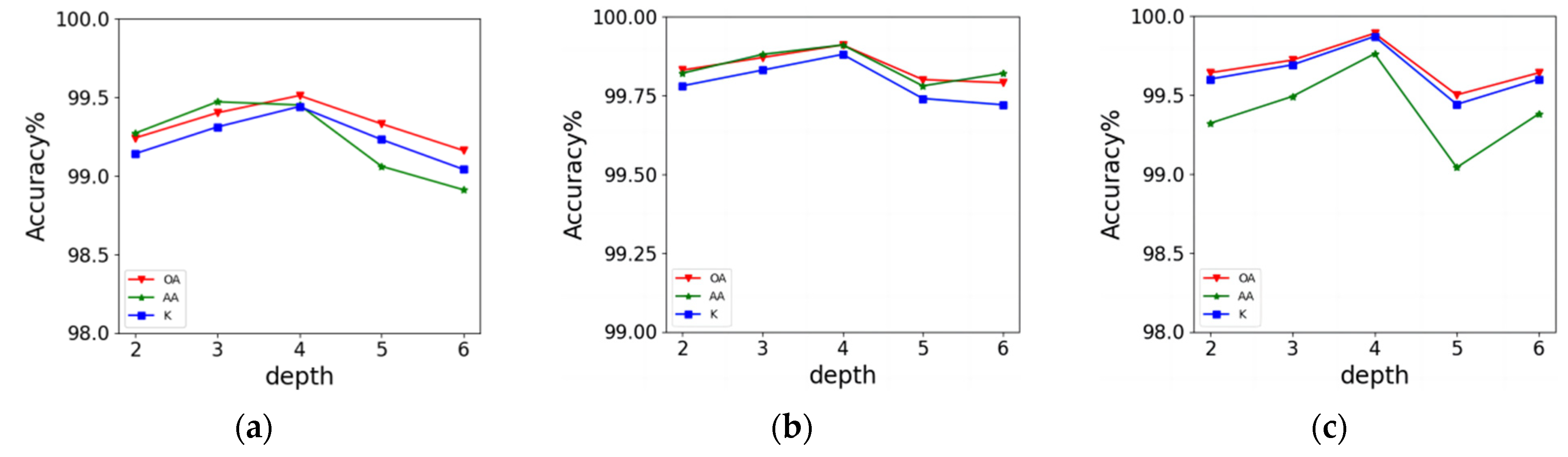
3.2.3. Effect of the Feature Extraction Structure Depth
The depth of the feature extraction structure also dramatically impacts the accuracy. As shown in
Figure 13, the classification results improved with the increasing depth of the feature extraction structure. OA reached the highest on three datasets when the depth was 4, which was 99.51%, 99.91%, and 99.89%, respectively. For all the datasets, the accuracies began to fall after depth 4. As shown in
Figure 12b,c, the classification accuracies on UP and KSC datasets are unstable. When the depth was 5, the OA decreased by 0.39% and 0.11% but improved by 0.14% and 0.04% when the depth was 6. Thus, we chose the optimal depth of the feature extraction structure of CA-FFDN to be 4.
3.2.4. Ratios of Training Dataset
The bigger the division ratio of the training dataset, the higher the classification accuracy. Different ratios of the training dataset are discussed in
Table 2 to select the optimal one. For all datasets, OA and training time increased along with the ratio of the training set, validation set, and testing set. For the IP, UP, and KSC datasets, OA reached 99% when the ratio was at 2:1:7, 1:1:8, and 2:1:7, respectively, which already met with the expected results of the experiment. In addition, OA reached 99.9% when the ratio was 5:1:4 for the IP dataset and 3:1:6 for the UP dataset. However, then came the increase in training time cost. Training the network took almost double the time when the training samples rose by 10%. Finally, we selected a ratio of 2:1:7 for the IP and KSC datasets and 1:1:8 for the UP dataset.
3.3. Ablation Experiment
To verify the effectiveness of SC-bottleneck (S), ECA-FF (E), and transition layer (T), we performed six groups of ablation experiments. As shown in
Table 3, the ECA was removed from the ECA-FF module in Group 1; the SC-bottleneck was not used in Group 2; the transition layer was not applied in Group 3; both the ECA mechanism and the SC-bottleneck were removed in Group 4, but the transition layer was retained; the transition layer was removed in Group 5 based on Group 4; and the sixth group of experiments is the proposed network in this paper. Each experiment was carried out ten times, and the average value was taken.
The experimental results on three datasets of Groups 1, 2, and 3 were compared with the results of Group 6, respectively, showing that the SC-bottleneck, ECA-FF module, and transition layers can improve the classification results. And the comparison of the results between the fourth and sixth groups shows that networks without transition layers decrease in accuracy, which verifies the applicability of adding transition layers in CA-FFDN. For the IP dataset, the fifth group of experiments achieved the worst classification accuracy, with a 0.3% decrease from the best result. For the UP dataset, Group 3 achieved the worst classification result. Still, in terms of the high spatial resolution of the UP dataset and the small number of mixed pixels, the classification accuracy reached more than 99.7%. Beyond that, the effectiveness of the ECA-FF module and the SC-bottleneck can be illustrated based on the comparison with Group 5. For the KSC dataset, the network lacking the ECA mechanism achieved the worst classification accuracy, and the OA was reduced by 0.44% compared with the best setting, and the ECA mechanism will significantly improve the classification accuracy of the KSC dataset.
To further prove that our attentional feature fusion strategy is more robust than other attention mechanisms. We employed channel attention mechanism (CAM), spatial attention mechanism (SAM), CBAM, and SENet to replace the ECANet in the ECA-FF module, respectively. It is observed from
Table 4 that SENet obtained the worst results among all attention mechanisms, and the reason was that the process of dimensionality reduction in the fully connected layers brought side effects to the extraction of channel information. All attentional feature fusion methods’ OA reached 99%, reflecting our network’s robustness. Meanwhile, attentional feature fusion based on ECANet outperformed other attention methods because ECANet can capture the cross-channel information to make full use of the semantic information.
3.4. Comparative Analysis of Classification Results
Five advanced networks were selected for comparative analysis, including 3D-CNN [
57], HybridSN [
58], 3D-SE-DenseNet [
34], MDSSAN [
50], and MSDN [
32]. The 3D-CNN contains three 3D convolutional layers and two global-pooling layers. Meanwhile, the dropout strategy is added to prevent overfitting. HybridSN is a 3D and 2D convolution combined network, which is more efficient than simple 3D-CNN networks. In the 3D-SE-DenseNet, each dense block is followed by an SENet structure, and both the dense blocks and dense layers were set to 3 in this paper. MDSSAN applies separable convolution in the bottleneck to reduce the training parameters. The depth of MSDN remained the same as ours. In order to ensure the fairness of the experiments, all experimental data were measured under the same environment, and the sample division ratio of different datasets, as well as input size for each network, were the same as ours. Furthermore, the optimal parameter settings of each network are consistent with those of the references.
Table 5,
Table 6 and
Table 7 show the classification results of the experiments, and
Figure 14,
Figure 15 and
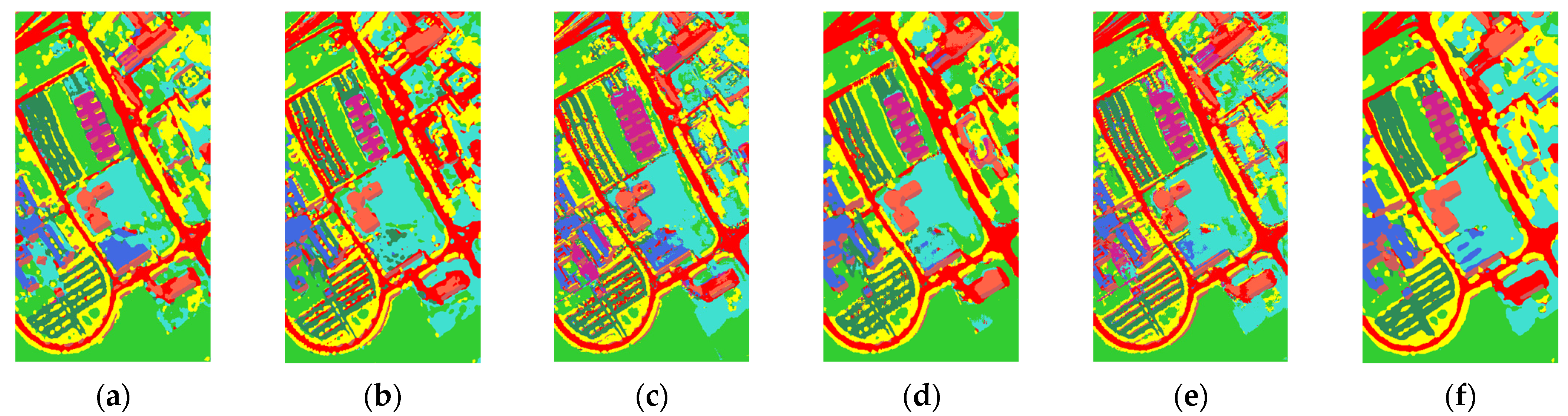
Figure 16 present the classification maps on three datasets.
The proposed CA-FFDN provides the best average results along with the highest OA, AA, and K values on all three datasets. For the IP dataset, compared with the five types of networks, 3D-CNN, HybridSN, 3D-SE-DenseNet, MDSSAN, and MSDN, the OA of CA-FFDN increased by 1.73%, 1.14%, 1.26%, 0.98%, and 0.45%, respectively; for the UP dataset, the OA of CA-FFDN increased by 0.91%, 0.87%, 0.60%, 0.31%, and 0.3%, respectively. For the KSC dataset, the OA of CA-FFDN increased by 2.01%, 1.08%, 1.65%, 0.97%, and 0.75%, respectively. We can note that 3D-CNN has the lowest classification accuracy compared to other networks on the three datasets. The reason is that the network structure of 3D-CNN is too simple to extract fine spatial–spectral features in most cases. The HybridSN combined comprehensive spatial and spectral information in the form of 3D and 2D convolution. Thus, it performed well in specific land cover, such as alfalfa and corn, on the IP dataset. 3D-SE-DenseNet and MDSSAN gradually refined the extraction of HSI features due to the consecutive dense block structure. Compared with 3D-CNN, the OA improved by 0.47% and 0.75% on the IP dataset, 0.31% and 0.60% on the UP dataset, and 0.36% and 1.04% on the KSC dataset, which indicated the effectiveness of dense networks, but they achieved lower accuracy in the classification of small sample categories, such as grass-pasture-mowed and sheets. The OA of MSDN was reduced by 0.45%, 0.30%, and 0.75% compared to ours on three datasets, respectively. By observing the experimental results, our network outperformed other networks, achieved the highest accuracy, and could quickly converge in fewer training iterations because introducing an efficient channel attention mechanism makes up for the underfitting of the network and preserves as much of the original semantics as possible by compensating for feature loss.
Figure 14,
Figure 15 and
Figure 16 present the classification maps on three datasets. The completeness of the classification maps remained broadly consistent with the classification results. In particular, 3D-CNN, HybridSN, 3D-SE-DenseNet, and MDSSAN had more noise and misclassification situations on the IP and KSC datasets. The MSDN achieved the fine classification of ground objects, while noise was also significantly reduced compared with the rest of the networks. CA-FFDN was the best regarding ground object classification, generating smoother results with few misclassified samples in classification maps. Due to the large sample size of the UP dataset, the obtained classification maps were relatively good, and there were few noticeable differences between the classification maps.
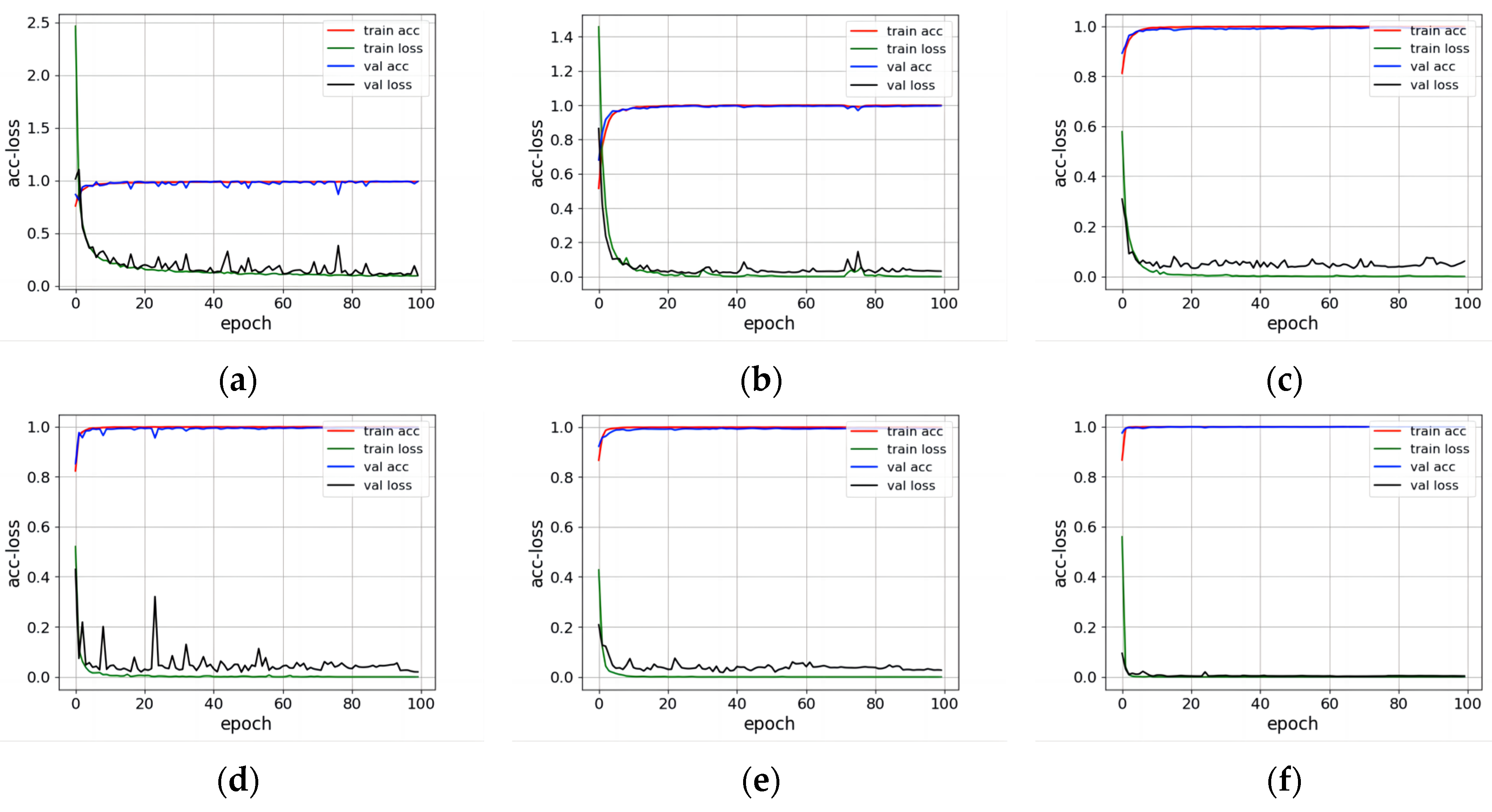
3.5. Comparative Analysis of Convergence Performance
To further evaluate the convergence performance of the proposed network, more experiments were conducted on each network on three datasets to obtain the accuracy and loss variation between the training and validation sets during the training process.
Figure 17,
Figure 18 and
Figure 19 portray that CA-FFDN had the slightest loss fluctuation in training and validation sets, and the network converged the fastest. In contrast, 3D-CNN had the slowest convergence speed during the training process because it generally lost important and detailed semantic information, which made it hard to converge fast. In particular, HybridSN was set with the largest batch size of 256 among all networks. Thus, more original data can be trained within a shorter time, which will lead to a fast convergence process. Both 3D-SE-DenseNet and MDSSAN adopt dense connection and attention mechanisms, and the accuracy and loss convergence speed of the training set were greatly improved compared with 3D-CNN.
Many factors can lead to loss fluctuations. The convergence speed of the MSDN was second only to CA-FFDN. Still, there were inevitable fluctuations in the validation set due to its complex network structure with a large number of parameters, so the network’s stability was not good enough. The reason why 3D-SE-DenseNet and MDSSN fluctuated severely on the IP and KSC datasets, compared with other networks, was unbalanced data division as well as small batch size. In other words, insufficient validation set samples and small batch size will lead to loss fluctuations. We also recorded each network’s parameters and training time in the training process, as shown in
Table 8. Compared with MSDN before improvement, CA-FFDN reduced the network parameters by more than half, and the training time was greatly reduced. At the same time, the accuracy and convergence speed of the network was guaranteed, which showed the effectiveness of the proposed network.
3.6. Comparative Analysis of Different Percentages of Training Samples
To further evaluate the generalizability of the proposed CA-FFDN, different percentages of the training samples were tested, 5%, 7%, 9%, 15%, and 20% for the IP and KSC datasets, and 0.5%, 1%, 3%, 5%, and 10% for the UP datasets. It can be observed from
Figure 20 that as the percentage of training samples increases, the overall accuracy of each network improves. In detail, MSDN performed worst when training samples were less than 15% on the IP dataset. 3D-SE-DenseNet also had the worst classification results in the case of small samples on UP and KSC datasets. Nevertheless, different networks performed differently on three datasets. But, in general, our CA-FFDN had the most robust performance under small training samples, which achieved the highest OA among all networks on three datasets.


