Analysis and Performance Evaluation of Transfer Learning Algorithms for 6G Wireless Networks

Abstract

The development of the 5G network and the transition to 6G has given rise to multiple challenges for ensuring high-quality and reliable network services. One of these main challenges is the emergent intelligent defined networks (IDN), designed to provide highly efficient connectivity, by merging artificial intelligence (AI) and networking concepts, to ensure distributed intelligence over the entire network. To this end, it will be necessary to develop and implement proper machine learning (ML) algorithms that take into account this new distributed nature of the network to represent increasingly dynamic, adaptable, scalable, and efficient systems. To be able to cope with more stringent service requirements, it is necessary to renew the ML approaches to make them more efficient and faster. Distributed learning (DL) approaches are shown to be effective in enabling the possibility of deploying intelligent nodes in a distributed network. Among several DL approaches, transfer learning (TL) is a valid technique to achieve the new objectives required by emerging networks. Through TL, it is possible to reuse ML models to solve new problems without having to recreate a learning model from scratch. TL, combined with distributed network scenarios, turns out to be one of the key technologies for the advent of this new era of distributed intelligence. The goal of this paper is to analyze TL performance in different networking scenarios through a proper MATLAB implementation.

1. Introduction

Through network programmability and integrated intelligence, 6G technology is expected to converge the digital, physical, and personal domains into a cyber–physical continuum [1]. Various innovative technologies, such as edge computing, the Internet of Things (IoT), and machine learning (ML), are expected to play a key role in enabling the 6G network. In recent times, advanced ML methods have been adapted to solve complex wireless networking problems effectively [2]. However, the traditional ML approaches, such as centralized ML techniques, suffer from several issues, particularly resource-constrained wireless networks. The unprecedented training time and associated costs are one of the main challenges that limit large-scale deployments of ML methods over wireless settings and can be a major obstacle in enabling full-scale distributed intelligence in 6G networks. Therefore, it is important to optimize the ML frameworks to improve their performance over resource-constrained wireless domains. Different ML frameworks are considered in terms of, e.g., distributed learning, multi-agent systems, hierarchical learning, and meta-learning, to effectively improve the ML training process [3,4,5,6].

Artificial intelligence (AI)-assisted 6G wireless communications is a burgeoning research area [7]. Some of the key benefits of exploiting AI in 6G networks are given as:

•

Improved spectral efficiency: AI can be employed to optimize the use of a spectrum in 6G networks, which could lead to increased capacity and improved performance [8].

•

Reduced latency: AI can be used to reduce latency in 6G networks, which is critical in many applications, particularly in real-time video streaming and autonomous driving [9].

•

Enhanced security: 6G network security can be improved by using AI, which is vital for preventing cyberattacks [10].

However, there are still a number of challenges that need to be addressed before AI can be fully deployed in 6G networks, including the following:

•

The necessity for large datasets: AI algorithms require large datasets for training, which could be challenging in 6G networks, where data collection may be difficult.

•

The need for high-performance computing: AI algorithms can be computationally expensive to run, which is potentially a challenge in 6G networks, particularly where computing resources may be limited. The authors in [11] discuss the difficulties of utilizing AI in enormous MIMO frameworks, for example, the necessity for huge datasets and the requirement of high-performance computing, and endeavor to recommend strategies to address these issues.

•

The necessity for security: AI algorithms could be susceptible to cyberattacks, a challenge that must be addressed before AI can be fully deployed in 6G networks. The authors in [12] address the security challenges of using transfer learning (TL) in 6G networks. The authors proposed numerous techniques to secure TL systems, such as using encryption and authentication.

Despite these difficulties, AI-supported 6G wireless communications is a promising field of study, as AI can make 6G networks even more powerful and efficient. This also motivates further exploration of the traditional ML-enabled approaches when implementing AI solutions.

Transfer learning (TL) is a recently introduced ML tool that can enable an efficient learning process over resource-constrained networks [13]. The key fundamental of TL is knowledge transfer (KT), corresponding to the utilization and transfer of knowledge and experience gained from similar source tasks in the past to facilitate the learning of new related target tasks. Thereby, TL approaches can increase the convergence rate, minimize reliance on labeled data, and improve the robustness of ML techniques in different wireless settings.

With the integration of IoT subsystems into wireless networks, an unprecedented amount of data are available at the network edge. However, these data are highly distributed, so using them for training centralized ML models through centralized server entities can be highly challenging in terms of resource requirements. On the other hand, with several new hardware innovations, the end devices are capable of training models effectively with onboard resources. This has enabled an edge intelligence trend to enable large-scale distributed intelligence. Although edge devices are capable of training ML models effectively, they still have limitations in terms of onboard resources. This limits their ability to train complex ML models such as deep neural networks (DNN). TL methods can reduce training costs for generic ML settings. TL can be effectively used to train complex DNN models with limited resources. Such a deep transfer learning approach has already gained some attention [14]. However, it is important to take into account the end devices’ capabilities, task features, available data, and several other factors while inducing the TL methods into deep learning techniques. These features can greatly impact the performance of deep TL models in training and test environments. Therefore, analyzing the performance of deep TL solutions with respect to the above-mentioned features can help us to understand the interesting trade-off between the performance measures and the device/network capabilities.

With this motivation in mind, in this work, we have analyzed the performance of the deep TL methods with respect to the memory requirements in terms of training data and the total number of layers selected for retraining the TL models for performing tasks that are different from the original one. A Matlab-based pre-trained SqueezeNet model is considered for performance analysis.

The main contributions of this work are:

• ML for 6G: Given the importance of distributed intelligence in the upcoming 6G systems, several ML frameworks are introduced and analyzed from a 6G perspective.
• TL Analysis: TL can be an important tool to enable distributed intelligence over resource-constrained wireless networks with an efficient training process. The different features of the TL methods and their impact on training environments are described in detail.
• Simulation Environment and Model: To analyze the performance of TL methods and the impact of its features in terms of layer selection, training data requirements, etc., a pre-trained SqueezeNet model in a Matlab environment is considered.
• Performance Analysis: With the considered SqueezeNet model, different simulations are performed by varying the number of training and data during the ML model training process. The proper analysis and conclusions are drawn from the studies performed.

2. Machine Learning for 6G

ML is a branch of AI that develops algorithms and models capable of learning from past experiences and data. It is essentially a form of applied statistics to estimate the performance of a target function designed for a particular learning task. The ML process involves several phases, including data collection and preprocessing, model selection and hyperparameter settings, model training and testing, validation, performance analysis, etc. In general, the model training procedure consists of identifying a function $f^p\left(w\right)$ (the cost function) for the task p with learning parameters, i.e., weights w, and finding the optimal value of w for which the cost is minimal, that is:

$$w^{*}=arg\; minf\left(w\right)$$

One of the most explored approaches is to use a gradient descent method that uses a gradient of a function f, $\nabla f$, to reduce the cost value (by moving in an opposite direction and updating the weight parameters) iteratively. In each step, parameters w can be updated as $w^{\prime }=w-ϵ(\nabla wf\left(w\right))$ [15] with $ϵ$ being the learning rate.

ML solutions can be classified into several groups, including supervised learning, unsupervised learning, semi-supervised learning, reinforcement learning (RL), etc. Supervised learning uses a labeled dataset to train the ML models, while unsupervised learning can work with unlabeled datasets. Additionally, RL agents aim to learn the optimal policies for selecting proper actions over unknown environment states through interaction and proper feedback. Several of these ML techniques can be used to solve complex wireless network problems. Some examples include device scheduling, resource allocation, congestion control, network routing, etc. [16].

In the case of wireless networks, end devices collect the data through different sensory nodes over time. ML methods can exploit such complex datasets to harness intelligence through pattern analysis. In the case of traditional ML frameworks, the data collected by the devices are often communicated with centralized servers with powerful computation hardware. The centralized server nodes then are able to build common and powerful ML models with adequate performances. Such an approach can be adequate when the end device data are of limited size and service requirements are less stringent. However, in recent decades, with the evolution of 5G technology, several new services and applications have been added with heterogeneous demands. In addition to the innovative IoT use cases and high-quality sensor nodes, the data quality and corresponding data sizes have changed dramatically. This limits the use of centralized ML frameworks to enable intelligent solutions in the different 5G domains. The upcoming 6G technology dreams of building a fully connected and intelligent world through connected intelligence. This can put a tremendous burden on a traditional ML framework, and innovative solutions are needed.

With such demands in mind, in recent times, different distributed learning methods have been proposed and analyzed over wireless settings for enabling large-scale intelligence [17]. Distributed learning methods allow the training of ML models in a distributed manner to reduce data collection and training costs compared to traditional ML methods. With several hardware innovations in the recent past, novel computation and storage hardware are present at the end devices, which can be exploited to train the ML model locally. Then, through collaborative mechanisms, the devices share their knowledge to generalize the training performance. This framework is often known as distributed learning. There are different types of distributed learning methods available, including federated learning, split learning, collaborative learning, multi-agent RL, etc. Although distributed learning methods such as FL have several advantages in terms of ML model training operations, data security, and energy efficiency, further performance improvements are still needed, in particular, for handling the large-scale distributed intelligence of 6G use cases. Advanced learning tools such as TL can be extremely useful to enable efficient distributed learning methods in resource-constrained 6G wireless environments.

TL is a type of learning that is based (as the term suggests) on a transfer of knowledge from one ML model to another. It is, therefore, a possible approach for the different learning categories: supervised, unsupervised, and reinforcement. The goal is to transfer knowledge from a designated learning model to solve a specific problem, called the source task, to another model thought to solve another one, called the target task. It is important to note that, in general, the performance of ML models is guaranteed by the hypothesis that the training set has the same probability distribution as the test set. Therefore the training data must be independent and identically distributed with respect to test data; in other words, the probability distribution that generates the training data must be the same one that generates the test data. The advantage of using TL comes from the fact that this hypothesis cannot necessarily be respected a priori but is achieved due to the TL itself [14].

Let us now explore a little more in detail the TL, introducing the concepts of domain and task, necessary for understanding the more formal definition of TL, in which we have two models, and one of the two must transfer knowledge to the other. A domain consists of two elements:

• A feature space $\mathbf{X}=\left\{X_i\right\}$, with $X_i=x_1,\cdots ,x_k,\cdots ,x_K$ with all data classes.
• A marginal probability distribution of $X_{i}P\left(X_i\right)$.

Given a domain, a task is also defined in two parts:

• A label space L.
• A predictive function $f\left(\right)$ that is learned by the relation $x_i$ and $l_i$ with $x_i\in X,l_i\in L$.

Hence, a task is composed as $T=\{L,f(\left)\right\}$. For more clarity, the function $f\left(\right)$ can be defined qualitatively as:

$$f\left(x_i\right)=\{P\left(l_k\right|x_i)|l_k\in L,k=1\dots \left|L\right|\}$$

which is the conditional probability that $x_i$ belongs to a certain class [18]. Always keeping in mind the scenario in which a knowledge transfer takes place, we consider a starting domain (source):

$$D_s=\{(x_{s_1},l_{s_1}),\dots ,(x_{s_i},l_{s_i}),\dots ,(x_{s_{n_s}},l_{s_{n_s}})\}$$

with $x_{s_i}\in X_s,l_{s_i}\in L_s$. We also consider a target domain:

$$D_t=\{(x_{t_1},l_{t_1}),\dots ,(x_{t_i},l_{t_i}),\dots ,(x_{t_{n_t}},l_{t_{n_t}})\}$$

with $x_{t_i}\in X_t,l_{t_i}\in L_t$. In the considered case, the number of instances in the target domain is definitely much lower than that of the source domain (we have a small dataset on which to train the network) or $0\le n_t\le n_s$.

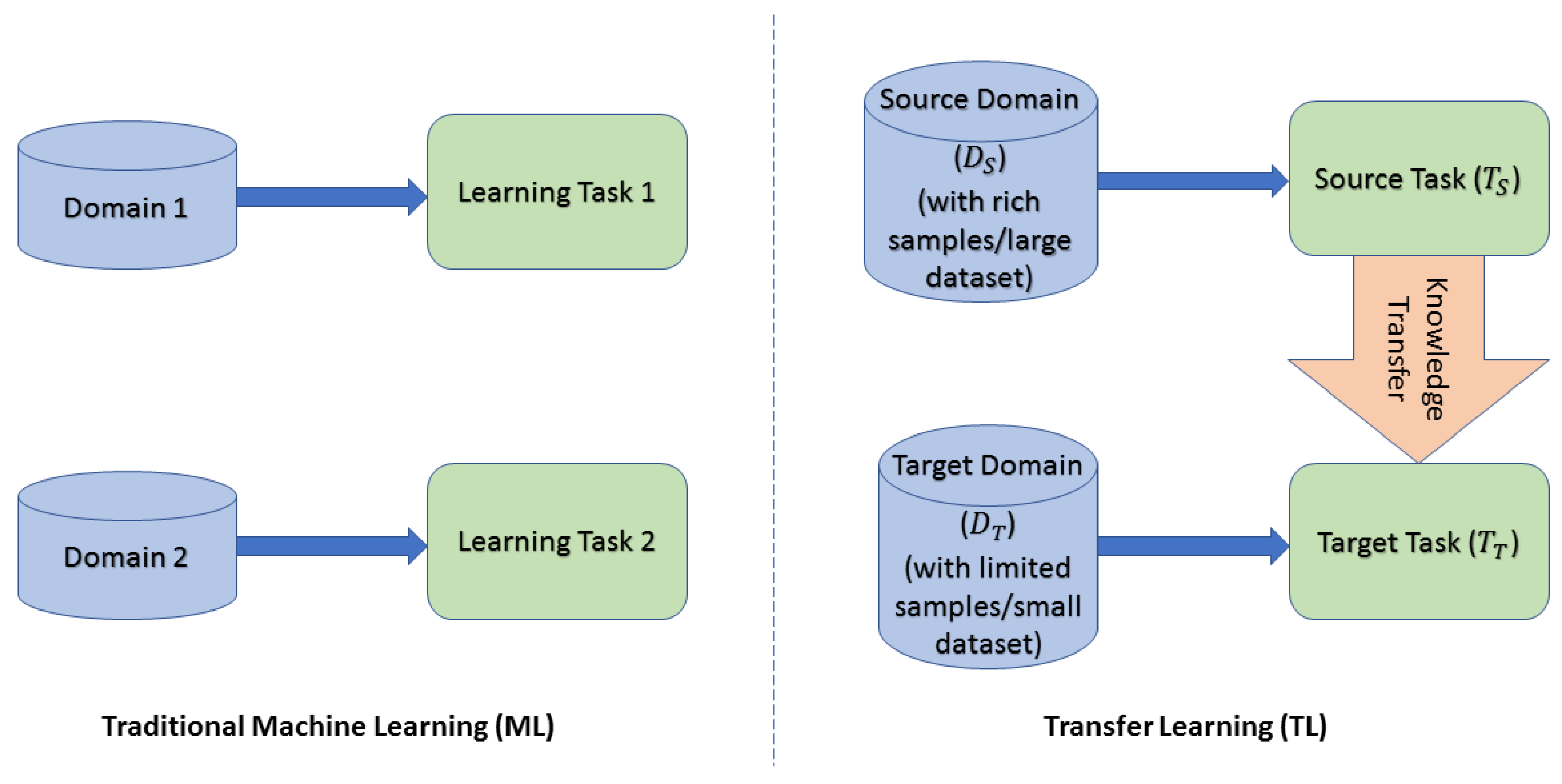
With TL, the learning process of the target domain can be improved by exploiting the transfer of “knowledge” from the source domain, as represented in Figure 1. It is, therefore, possible to give the most rigorous definition of TL [18]:

Given a $D_s$ source domain with its source task $T_s$ and a target domain $D_t$ with respect to target task $T_t$, the goal of TL is to learn the target $f{\left(\right)}_t$ predictive function using the knowledge acquired by $D_s$ and $T_s$ in a situation where $D_s\ne D_t$ or $T_s\ne T_t$.

Feature extraction and fine-tuning are the two primary types of TL. In the feature extraction TL, a previously trained model in the source domain is used to extract features from the new target dataset that will later be used to train the new target model for the specific target task, whereas, in fine-tuning, the pre-trained model’s weights are slightly adjusted on the new target data to improve the performance or accuracy of the target task in the target domain. There are several advantages to using TL over traditional ML:

• Save time and resources: Gathering and labeling a large dataset for a new task is unnecessary,
• Enhance performance: The pre-trained model has already learned to extract relevant features for the new target task,
• Transfer knowledge across different domains: e.g., a model previously trained to recognize cars can be used to recognize trucks.

TL is specifically helpful in these applications:

• Image Classification (IC): A pre-trained model can be employed to extract features from new images, which can then be utilized to train a new model in a target domain for a specific classification task,
• Natural Language Processing (NLP): Acquires knowledge of the meanings of words and phrases to use in another NLP task, such as text classification or machine translation,
• Speech Recognition (SR): Learns the acoustic features of speech to use in other specific speech recognition tasks.

In conclusion, TL is a potent technique to enhance the performance of machine learning models, especially when limited data, samples, or labels are available for the target task.

2.1. Deep Learning

Deep learning techniques are expected to enable intelligent services in the upcoming 6G world. They are a subset of ML that focuses on using artificial neural networks to analyze and understand data. These neural networks are made up of many processing units (called neurons) organized in successive layers, which work together to recognize patterns and relationships within the data to provide an output based on the characteristics of the data input to them.

Deep feedforward networks, also called feedforward neural networks, are one of the most widely explored neural networks for different applications. In general, the feedforward network can be defined as $y=f(x,\theta )$, with $\theta$ representing a parameter or a set of parameters that needs to be optimized to have the best approximation of the function $f^{*}$.

Deep neural networks (DNN) can have an input layer, several hidden layers, and an output layer. The number of hidden layers depends on the complexity and behavior of the network and provides the overall length of the chain of functions or depth of the model. As for the design and training of a neural network, there are not many differences from what happens for any other model of ML. The gradient descent technique can be used to train DNNs. However, a DNN often requires an extensive amount of training data and resources for building a proper ML model with adequate performance. This limits the uses of DNN over highly distributed wireless networking scenarios where both data and device resources are limited. This opens a new door to improving the performance of the DNN training process through the integration of advanced tools such as TL. In fact, several forms of deep TL strategies were considered in the recent past through the integration of knowledge transfer procedures into DNN models.

The Deep TL strategies refer to the use (or better to the reuse) of pre-trained models to improve the DNN training process. In this regard, there are three types of TL techniques that use pre-trained models:

• Off-the-shelf pre-trained models: This category refers to DNNs that were already trained and used in the past for tasks having some similarities to the current learning task to exploit the previous knowledge. For example, if one aims to solve an image recognition problem, pre-trained neural networks such as GoogleNet or VGG can be used to achieve good levels of accuracy. However, in practice, it is difficult to find pre-trained models that fit perfectly into new tasks without making any changes. Even small differences between the domain and the source task and the domain and the target task can have a huge impact on the performance, and that makes this method ineffective in many cases.
• Pre-trained models as feature extractors: The problem encountered before in the off-the-shelf pre-trained models case can be tackled through the use of pre-trained models as feature extractors. Traditional ML algorithms, such as classification and regression, require a data pre-processing step in order to extract the main features to be able to train the model effectively. In many occasions, this procedure can take a long time and many resources if performed manually. The ability of a neural network to extract characteristics can be helpful in such situations to make the feature extraction process automatic. In this case, neural networks can only extract characteristics of the target domain that can be applied to generic problems. The target data can be processed by the network for highlighting and extracting features. These features can then be, for example, further elaborated by a regression or classification model to output the number or category to which the “raw” data belongs at the beginning [18].
• Fine-tuning of pre-trained models: This technique allows the portion of the network to be trained by using data from the target domain in order to have a task-specific model enabled through “transferred knowledge” [18]. This can be achieved through the following procedures:

  (a)

  Weights initialization: In this case, the parameters of the target model are initialized with the values of the pre-trained network, after which the network is trained using all the target domain data. This procedure is adopted when there are many available data in the target domain.

  (b)

  Selective fine-tuning: In this procedure, the model parameters are initialized to the values of the parameters of the pre-trained network as in the previous case. However, only part of the network is trained. Some layers of the network are frozen during the new training phase, and consequently, the weights related to these layers are not updated. The logic that can lead to a correct selection of levels to freeze depends on how similar the tasks of the source and destination are. In general, the first levels of a neural network extract low-level features, while the deeper levels capture more high-level features, such as shapes and objects, giving rise to a hierarchical extraction of characteristics. Therefore, if the problem to be solved is similar to that for which the network was pre-trained, only a few layers can be trained, while if the two problems are rather different from each other, it may be necessary to use several layers for the new network training.

2.2. Transfer Learning in 6G Scenarios

TL can enable intelligent solutions in the 6G world, particularly to enable large-scale distributed intelligence, with particular attention to the IoT subsystem characterized by resource-constrained devices. However, IoT systems often have resource limitations, heterogeneous natures, and data diversity. Therefore, TL solutions should be adapted according to the characteristics of different IoT systems and user demands. TL can be an effective tool for enabling high-quality ML models with a reduced amount of data. An example is the compressed sensing (CS) technique, which is considered in 6G-IoT scenarios to reduce the transmission overhead for high-dimensional IoT data. The performance of CS techniques can be enhanced through deep-learning-based CS approaches. However, such complex learning methods often demand a large amount of training data, which can be difficult to produce. In [19], authors have studied such deep-learning-based CS solutions and applied TL to counter the challenges. The importance of TL from the 6G network perspective is analyzed in [20], including the possible modifications required in 6G network architecture to adapt TL solutions. In [21], authors proposed a TL-enabled deep learning solution for 5G industrial edge networks for optimizing the device latency and energy performance with limited resources. A detailed review of TL solutions that can be effectively used in 6G networks is provided in [13], along with the example scenarios and possible challenges to be considered. In [12], authors have proposed TL-based solutions for the case of the 6G-enabled Internet of Vehicles. In addition, they analyzed the security issues and proposed a secure and reliable TL framework with the help of blockchain technology. The network slicing approach is an important aspect to consider in 5G and beyond 5G networks to enable heterogeneous services simultaneously [22]. In [23], authors have proposed a TL-based deep RL solution for RAN slice resource allocation.

Moreover, there are some specific 6G scenarios where TL seems to impact a lot with its characteristics. In the following, we have summarized several TL-based solutions for non-terrestrial networks (NTN) and industrial IoT cases. Both of these frameworks can be extremely useful in the upcoming 6G world, and integrating proper TL solutions over them can be highly recommended.

2.2.1. TL for Non-Terrestrial Networks

Various air- and space-based NTN platforms are expected to play a key role in enabling a fully connected and intelligent 6G world [24]. NTN platforms can boost the coverage and capacity of terrestrial networks. In addition to this, NTN platforms can also enable edge computing in the space through the onboard deployments of storage and processing units. With the onboard computation and storage resources, NTN platforms can enable various intelligent services in the space. However, with their limited size, NTN platforms can only have a limited number of services onboard. Based on the user demands and other local environment characteristics, it is important to optimize and update the services over such resource-limited NTN nodes. Such optimal service placement problems can be solved through different ML methods for enabling intelligent solutions. However, such solutions can be computationally expensive, platform dependent, and may require frequent retraining, mainly due to the dynamic behaviors of NTN nodes. Performing the ML model training from scratch can be costly or even infeasible with the limited NTN resources. In such scenarios, TL can be extremely useful in performing efficient ML model training operations.

In [25], the authors have proposed a distributed multi-agent learning solution for service scheduling over UAVs. In particular, the performance of independent and transfer-learning-based solutions is compared to show the various advantages in terms of resource requirements, overall performance, etc. Furthermore, in [26], the authors have proposed a joint UAV deployment and resource allocation scheme based on TL methods. The space-based computation environment can also be exploited for processing user data through a computation offloading process [27,28]. However, given the limited computation resources, optimizing the amount of data to be offloaded to each edge server is important. Such computation offloading problems can be solved through innovative ML-based solutions. However, it can induce large training overheads. TL can be explored to provide efficient ML solutions for computation offloading problems. For example, in [29], the authors have proposed RL-based solutions for the computation offloading problem and used TL to optimize it further. Such studies need to be analyzed further by taking into account the diverse nature of NTN nodes, resource limitations, data diversity, etc., to further improve the performance of TL solutions in space.

2.2.2. TL for Industrial IoT

The industrial Internet of Things (IIoT) is another important usage case that can be extremely useful in the 6G world for automating different industrial processes. In particular, different ML solutions can be adopted over IIoT environments to enable intelligent solutions. However, data scarcity and the unavailability of quality data can limit ML applications over IIoT scenarios. In such cases, TL methods can be adapted to enable intelligent solutions. In [30], a broad analysis of the applicability of TL solutions in IIoT scenarios is provided, including work principles, main challenges, and building blocks. Data privacy can be another challenge that can reduce the applicability of traditional ML solutions in IIoT environments. In [31], the authors have proposed federated transfer-learning-based solutions for smart manufacturing problems. With the added advantage of federated learning and TL, such solutions can enable efficient and private learning processes in IIoT environments. Apart from data availability, the limited computation capabilities of IIoT nodes can also impact the ML adaptation process in IIoT. In [32], the authors have discussed such issues and proposed deep TL solutions to reduce training overhead. Similar to the NTN case, the IIoT environment is filled with heterogeneous and resource-constrained devices with limited data. Optimizing the TL solutions to provide appropriate learning frameworks based on the IIoT environment characteristics can be highly useful.

2.2.3. TL Testbeds in 6G and B5G Scenarios

The application of TL can be effectively executed in real-world scenarios by taking into account the subsequent factors:

• The hardware requirements: TL necessitates a robust computing infrastructure to train and deploy deep learning models. This could pose a challenge in resource-constrained environments. Furthermore, since 6G networks must support a wider variety of applications, especially AI-based applications, their hardware requirements are significantly higher than those of the current 5G networks.
• The infrastructure necessary to support AI: 6G networks will have to be able to support the high bandwidth and low latency requirements of AI-based applications. This will necessitate significant investment in network infrastructure. The authors in [20] discuss the hardware and infrastructure requirements for TL in 6G networks, and propose a number of techniques to improve the efficiency of TL, such as using quantized neural networks and caching the models in the edge devices.
• The similarity between the source and target tasks: The success of TL greatly depends upon the similarity of the source-target domains and/or tasks. If the tasks/domains are too different, TL may not be effective [33].

2.2.4. Contribution with Respect to the State-of-the-Art

Though the above-mentioned TL-based studies are able to improve the learning performance in different dimensions, further optimization is needed. Several of these past studies where TL-based solutions are applied to increase learning efficiency are not taking into account the heterogeneity of devices in terms of computation resources, training data, etc. These factors can have an impact on the TL performance, especially in the case of diverse IoT devices. Therefore, it is important to study the TL solutions’ performance in different training environments to cope with the system-level restrictions in the upcoming era of 6G networks. It is essential to examine the training performance of TL solutions with different levels of training data. Additionally, it is also important to analyze the performance of TL solutions based on the number of layers selected for the training process. Moreover, it is also important to analyze the impacts of the number of layers selected and the level of fresh data available for mode training operations.

The current state-of-the-art technology presented lacks in in-depth analysis of TL solution performance, and thus, there is a scope to further enhance the TL solution performance with such studies. Moreover, this kind of analysis can be an important step to further optimize the TL solutions and provide adaptive TL-based training frameworks over diverse IoT environments in the 6G networks. Therefore, in this article, we first consider the TL solution based on the SqueezeNet model for image data analysis. We analyze the performance of the SqueezeNet-based TL method for the image data classification problem. Next, we provide several simulation results showing the impacts of the training layer selection policies and the different levels of training data over the learning process. Furthermore, the simulation results are discussed in detail and proper remarks are presented in the discussion section. Some examples of 6G IoT scenarios are also presented in the discussion section where such analysis can be helpful. Moreover, further future directions for the studies performed are also highlighted in the conclusion section.

3. Experimental Setup for TL Performance Evaluation

The main aim of this work is to analyze the performance of deep TL techniques through experimental simulations. We have considered a well-known image classification problem and aim to build a DNN model through knowledge transfer. The experiments are performed over a Matlab-based simulator using a pre-trained SqueezeNet model. A proper image dataset containing 10 different classes of fruits is used [34]. The experimental analysis is based on the following two problems:

• Number of training levels: In general, wireless nodes can have limited training resources, limiting their ability to train DNNs. For the case of deep TL, a set of layers from a pre-trained DNN can be retrained over a fresh dataset for solving the new task. The device’s ability and task requirements can impact the number of layers selected for pretraining. Selecting a limited number of layers can reduce the overall performance of the DNN when applied to a new task. However, if an unprecedented amount of layers are selected to train again with fresh data, the overall training process can be prolonged, reducing the chances of satisfying the service demands. Thus, it is extremely important to analyze the performance of deep TL methods to find a suitable number of layers to be trained.
• Amount of training data: Another interesting factor that affects the deep TL process is the amount of data available. With the integration of IoT nodes with heterogeneous characteristics, wireless nodes are highly diversified. Different devices can collect and store a different number of data samples and can have differing data qualities. The amount of data available for retraining operations can highly impact the DNN training process. The proper number of DNN layers should be considered based on the available datasets to avoid issues such as underfeeding, overfeeding, etc.

SqueezeNet is a convolutional neural network (CNN) that represents the pre-trained model for image classification problems [35]. It is developed for image-processing applications on mobile and embedded devices. SqueezeNet’s distinctive feature is its highly compressed network architecture, which allows it to achieve high performance, comparable to networks with a much more complex nature with a relatively small number of parameters.

In general, CNN is an artificial neural network designed to process data with a grid structure, such as images. This type of network was developed to solve problems of classification and detection of objects in images. The basic structure of a CNN includes three types of layer sets: (i) convolution layers, (ii) pooling layers, and (iii) fully connected layers.

• Convolution layers are the core of CNN and are composed of a set of filters, each designed to detect a particular characteristic of the image in input. Each filter is mixed in the input image, calculating the sum of the products of the filter elements and the corresponding image pixels. This process produces a feature map (feature map), which is passed to the next layer [15].
• The pooling layers are used to reduce the size of maps in the characteristics. Pooling is performed using a preset size window, which slides over the input image and calculates a statistic on each window region, such as the maximum or average value. This reduces the amount of data that need to be processed in subsequent layers and helps prevent overfitting.
• Fully connected layers are used for the final classification. These layers receive in input the representation of the characteristics calculated from the previous levels and produce a distribution of probabilities on the possible outputs of the CNN.

SqueezeNet—A DNN Model for Image Data Analysis

The SqueezeNet model consists of 18 layers in total, of which 14 are convolutional layers and the other 4 are fully connected layers. It is important to note that the SqueezeNet version developed in Matlab as a pre-trained model contains more layers than the original, totaling 68 levels.

The sequence of levels that distinguishes SqueezeNet is called the Fire module. This module is a block of operations that takes an input tensor and returns an output tensor. It consists of two main layers, a compression convolution layer (squeezing), and an expansion layer (expanding). The compression layer consists of convolutions with $1\times 1$ filters and aims to reduce the number of input channels, thus, obtaining a compressed representation of the information. This helps to reduce the number of parameters needed for the network and improve computational efficiency.

The expansion layer consists of a combination of $1\times 1$ and $3\times 3$ filters and is intended to increase the number of input channels and, consequently, the information represented. The use of $1\times 1$ filters is to provide more flexibility for the network to control the number of output channels for subsequent layers [35].

The size of the filters in the expansion and compression layers are adjustable parameters of the Fire module and are $s1\times 1$, $e1\times 1$, and $e3\times 3$. In particular, $s1\times 1$ is the number of filters in the compression layer (all $1\times 1$), $e1\times 1$ is the number of filters $1\times 1$ in the expansion layer, and $e3\times 3$ is the number of $3\times 3$ filters in the expansion layer.

When using Fire modules, it is important to set the value of $s1\times 1$ less than the sum of $e1\times 1$ and $e3\times 3$ to limit the number of input channels for $3\times 3$ filters and then check the number of parameters needed for the network [35].

In general, the ML model performance can be modeled by using the concept of the capacity of the model. In particular, the main challenge of an ML and deep learning model is to be able to have an optimal performance in the presence of unknown data that have not yet been observed, especially during the training process. This feature is called generalization and can be estimated by calculating the error on a data set other than the one used for training, i.e., the test set, and the corresponding error is called the test error. During the training phase, error measurements can also be made using the training set. For example, using a subset of the data to see the model in action. The error generated by this measurement is called a training error, given the origin of the data. From this, it turns out that the capacity of the model can be estimated from these two aspects:

• ML models that have a reasonably small training error during the training process.
• ML models that have a small difference between training and test error (generalization gap).

The imperfect training process with large training errors can induce the problem of underfitting, while with the high generalization gap, trained models can have an overfitting problem [15]. The capacity measure can be defined as the ability of a model to adapt according to the underneath function. Therefore, it is the space of the functions over which the model can use to make predictions with proper performance.

Several factors can impact both training and generalization gaps. In particular, in the case of deep TL, the number of layers selected to pre-train (L) can increase/decrease the error values. Additionally, the total amount of data considered in terms of memory space M can also affect training/test performance. In the following, we introduce the minimization problem, which aims to minimize the training error and generalization gap error values as a function of L and M in deep TL models. The problem is defined as follows:

$$\mathbf{P}\mathbf{1}:\underset{\mathbf{L},\mathbf{M}}{min}{E}_{tr}(L,M)$$

(1)

$$\mathbf{P}\mathbf{2}:\underset{\mathbf{L},\mathbf{M}}{min}{G}_{tr}(L,M)$$

(2)

where training error $\left(E_{tr}(L,M)\right)$ and generalization gap $\left(G_{tr}(L,M)\right)$ are defined as a function of L and M.

4. Methodology for Performance Evaluation

For the case of model training operations, the image dataset is considered split between training and test data. Next, to measure the impact of memory size M, that is, the amount of data in terms of memory space, we have further divided the training dataset into several forms in terms of the percentage number of samples used from the original training data. In particular, we have defined 20 datasets of different sizes. The smallest dataset contains $5\%$ of data samples from the original training data, while the largest data set contains all the training data from the original data source. The other datasets have $5\%$ incremental data samples compared to the previous one.

We have considered different layer selection options to measure the impact of selected layers L. In particular, the 68 layers of the Matlab-based SqueezeNet network are considered during the knowledge transfer operations. Different levels of training operations, i.e., from low to high, are considered based upon the layer selection policies for the knowledge transfer and/or the training process. We have considered 10 different configurations of active levels, defined as $\mathrm{active}\mathrm{levels}\mathrm{for}\mathrm{training}=[5,12,19,26,33,40,47,54,61,68]$.

These levels were chosen in relation to the position of the convolution levels within the SqueezeNet network present on Matlab to extract different characteristics from the images. The code used in the Matlab simulation for the dataset import (training and testing) and subsequent dataset partitioning is resorted in Listing 1.

Listing 1. Dataset import and partitioning in Matlab.

fruit_train=imageDatastore(′C:\Users\nicco\Downloads\archivio\MY_data\train′,′IncludeSubfolders′,true,′LabelSource′,′foldernames′); fruit_test=imageDatastore(′C:\Users\nicco\Downloads\archivio\MY_data\test′,′IncludeSubfolders′, true, ′LabelSource′,′foldernames′); new_fruit_train = shuffle(fruit_train); new_fruit_test = shuffle(fruit_test); net = squeezenet; inputSize = net.Layers(1).InputSize; new_augimdsTrain = augmentedImageDatastore(inputSize(1:2),new_fruit_train); new_augimdsTest = augmentedImageDatastore(inputSize(1:2),new_fruit_test); data_partition = cvpartition(numel(indeces),′holdout′,0.2); tenperc_Trainingds = subset(new_augimdsTrain,training(data_partition)); tenperc_Validationds = subset(new_augimdsTrain,test(data_partition));

The image Datastore function [36] allows for the storage of a dataset containing images, and the additional inputs within the function served to import the labels of the images. The two lines of code after the dataset import were introduced to mix the data through the shuffle [36] function. After that, a pre-trained SqueezeNet [37] network was added. Additionally, the input layer is defined as $[227\times 227\times 3]$ which is also the input image size. The cvpartition function is used to divide the dataset into different sizes with random samples selected from the original data.

For the model training, the following procedure was carried out. For each different training set, 10 different nets were trained using the different active layer configurations mentioned before.

The pretrained model of SqueezeNet is able to perform classification on a problem of 1000 classes. However, the new task aims to perform the classification on a problem of 10 classes. To this end, the appropriate changes should be made, especially from the output side. These changes are performed over the last convolution layer and the classification layer form predicting the outputs that are different classification from the pre-trained network. Next, the training process is performed through the Matlab Script in Listing 2.

Listing 2. Training Process Script in Matlab.

%networks training i = 0; for j=1:10     layers(firstUnFrozen(j):63)=unFreezeWeights(layers(firstUnFrozen(j):63));     lgraph=createLgraphUsingConnections(layers,connections);     i = i+1;     switch i         case 1             network5_full = trainNetwork(full_Trainingds,lgraph,options);         case 2             network12_full = trainNetwork(full_Trainingds,lgraph,options);         case 3             network19_full = trainNetwork(full_Trainingds,lgraph,options);         case 4             network26_full = trainNetwork(full_Trainingds,lgraph,options);         case 5             network33_full = trainNetwork(full_Trainingds,lgraph,options);         case 6             network40_full = trainNetwork(full_Trainingds,lgraph,options);         case 7             network47_full = trainNetwork(full_Trainingds,lgraph,options);         case 8             network54_full = trainNetwork(full_Trainingds,lgraph,options);         case 9             network61_full = trainNetwork(full_Trainingds,lgraph,options);         case 10             network68_full = trainNetwork(full_Trainingds,lgraph,options);     end end

    The unFreezeWeights function [37], is used over the levels that were previously frozen in the network in order to use them for training. Different memory sizes are used to train the networks.

In the test phase, the training error was first calculated by evaluating the error over each network instance on the relative validation set. The script in Listing 3 is used to calculate the training error and the test error.

Listing 3. Training error and test error evaluation in Matlab.

load(′Big10%ofdataset_trained_networks.mat′); width = 10; training_error10 = zeros(width,1); test_error10 = zeros(width,1); Classnames=[′Apple′;′avocado′;′Banana′;′cherry′;′kiwi′;′mango′;′orange′;′pinenapple′;′strawberries′;′watermelon′]; y_true = readLabel(tenperc_Validationds.Files,Classnames); y_true_test = readLabel(new_augimdsTest.Files, Classnames); y_pred = classify(network5_ten,tenperc_Validationds); y_pred_test = classify(network5_ten,new_augimdsTest); L = logical(y_pred ∼= y_true); training_error10(1) = (numel(y_pred(L))/numel(y_pred))*100; L = logical(y_pred_test ∼= y_true_test ); test_error10(1) = (numel(y_pred_test(L))/numel(y_pred_test))*100;

The readLabel function [37] is used to assign the corresponding label to the images contained in the dataset in order to test the model. The classify function [37] is also considered to perform the classification, taking the input parameters from the trained network and categorical data to be classified.

5. Numerical Results

The test results were analyzed using a polynomial regression model. In order to view the data and understand the reciprocal relationships between them, we decided to explore a multivariable regression model that could express, in the form of a surface, the dependence between the number of levels used for the end-tuning, the memory needed to train the model vs the training error in one case, and the difference between training error and test error (generalization gap) in the other. In general, the regression function can be defined as $Z=f(x,y)$.

For example, z can represent the training error/generalization gap, being a function of the amount of memory, and the number of layers designated for training. Due to the noise between the results and the dependence on two variables, it is difficult to understand their impact on each other without such functional relationships between dependent and independent variables. Figure 2 shows the impact of memory size and the layer selections over the training error values in the form of surfaces.

Notably, in order to visualize such plots with complex interdependencies, a polynomial regression problem between two variables needs to be solved by using the performance data collected for different cases. Given the relatively small number of observations, the quadratic polynomial regression equation is considered, to avoid overfitting problems. It represents the value of the dependent variable less than an error. The relation is, therefore, the following [38]:

$$Z_i=b0+b1x_i+b2y_i+b3x_i^2+b4y_i^2+b5x_i{y}_i+e_i$$

The problem includes determining the value of the coefficients of the function that minimize the error in the prediction; for this, we have used the cost function defined as the mean squared error (MSE):

$$\frac{1}{n}\sum _{i=1}^n{e}_i^2=\frac{1}{n}\sum _{i=1}^n{\left(Z_i-\left(b0+b1x_i+b2y_i+b3x_i^2+b4y_i^2+b5x_i{y}_i\right)\right)}^2$$

To find the minimum of this function, we must derive the function for each coefficient and put it equal to zero; then, it is sufficient to solve the linear system containing the 6 equations described. The areas obtained are, therefore, two:

• a surface expressing the relationship between the number of levels for training x, the memory needed to train the y model, and the training error $z(x,y)$, as represented in Figure 3.
• a surface that expresses the relationship between the number of levels for training x, the memory needed to train the y model, and the gap generalization $z(x,y)$, as represented in Figure 4.

It is possible to analyze the projection of the surface both on the plane $(x,z)$ and $(y,z)$, in order to make considerations on the results obtained. Initially, we evaluated the case of the plan $(y,z)$, of the training error/generalization gap, as a function of the number of layers used to train the model. Then, we carried out the same analysis for the plan $(x,z)$ to study the dependence on the amount of memory used, in relation to the two functions considered.

• Case 1: the $y-z$ plane analysis

The generalization gap shown in Figure 5 has a large area between the maximum and the minimum value for each level, and one can notice that the area is maximum at the highest number of levels. This, therefore, means that the generalization gap can be impacted largely by the increasing number of levels. The highest gap value is 22.3% near the trained network instance, having all levels thawed, and the minimum gap in value, 7.8%, is in the vicinity of the case where the number of inactive layers is equal to 61 (i.e., complete training).

In the vicinity of a smaller number of frozen layers, however, the difference between the maximum and minimum gap decreases, allowing us to limit the damage in the ability to generalize new data. We define $X_{min}$ as the amount of memory associated with the minimum generalization gap and $X_{max}$ as the amount of memory associated with the maximum generalization gap; therefore, one can have:

$$\frac{dZ(X_{max},Y)}{dY}<-\frac{dZ(X_{min},Y)}{dY}$$

Therefore, using multiple layers for training does not bring benefits in this case, because it induces the risk of having a performance that is not adequate for the workload associated with the training process. It can increase the capacity of the model and lead to overfitting, i.e., the network is training on new data and loses the ability to generalize. The same consideration may be carried out for the case of the training error (in Figure 6), and in this case, it is notable that the minimum function occurs in the intermediate case of 47 levels used with an error of 4.8%.

• Case 2: The $x-z$ plane case

For the case of the $x-z$ plane, it can be seen that the generalization gap (as in Figure 7) becomes high when the amount of training data is increased, denoting a tendency of the model to induce overfitting issues more than underfitting.

Regarding the case of the training error (in Figure 8) instead, an underfitting trend with less than 50% of the dataset can be noticed, as well as an overfitting risk for data close to the full dataset size.

6. Discussion

The upcoming 6G technology is expected to demand large-scale distributed intelligence networks with extremely high performance. The TL methods can surely enable the efficient learning process by allowing pre-trained networks to be used for new tasks through different knowledge transfer mechanisms. However, the performance of TL solutions can be impacted by several factors, such as the number of layers considered for retraining, the amount of data available, the device capabilities, etc.

In this work, we have analyzed the performance of the deep TL model for understanding the impact of the number of layers selected and the considered amount of data for the training operations. It can be seen that using an unprecedented amount of data with a limited number of layers to be trained can badly impact the performance of the retrained DNN model. On the other hand, retraining a large number of network layers from a pre-trained TL model with a reduced amount of data can also induce several issues. Therefore, it is highly important to select the optimal number of layers to be trained and/or the amount of training data to be considered for retraining the models to be used for new tasks.

The proposed analysis of the TL performance can be used to understand the impact of different training mechanisms adopted during the integration of TL solutions, in particular, for the case of resource-constrained IoT devices in next generation networks. Moreover, 6G technology is expected to span several IoT usage cases with reduced-capacity devices, in particular, to enable distributed intelligence. Several of these IoT paradigms can benefit from enabling the proper TL-based learning solutions with enhanced performance. Some of these are listed below.

Vehicular IoT: To enable the autonomous driving case in the next generation of vehicular networks with the help of various IoT nodes and different communication mechanisms requires large-scale ML solutions. Such a vehicular paradigm can benefit from the proposed TL solutions, in particular, to analyze the distributed vehicular data. The inherent dynamicity, unstable communication environments, limited datasets, and on-board resources are some of the major challenges in vehicular networks. With this, enabling fully autonomous driving scenarios can be challenging with traditional learning methods. With the use of TL approaches, in particular, those that can adapt according to the vehicular nodes’ limited capabilities and datasets, can be highly effective.

NTN IoT: The satellite IoT is another important communication paradigm that is expected to play an important role in 6G networks to enable the intelligence in air and space technology for several different types of users. However, the limited on-board computation resources in satellite networks can be challenging to enable these intelligent solutions with the appropriate performances. The TL methods can be applied over satellite networks to enable efficient learning processes to analyze the satellite IoT data. The proposed studies can be important to understand the impacts of different TL solutions according to the varying datasets and the learning processes.

Industrial IoT: With the help of industrial IoT data and 6G technology, various industrial processes are expected to be optimized, automated, and revolutionized. The distributed learning solutions, enabled through small-scale datasets generated by different industrial IoT devices, are expected to play a key role. However, with such limited datasets, it is important to optimize learning frameworks to enable proper solutions. The proposed ideas of TL solutions and the analysis of the impacts of varying datasets over the TL performance can be useful during the application of TL solutions in industrial IoT paradigms.

The considered studies can further be explored in other dimensions to analyze the impacts of device capabilities, learning environments, and other similar aspects on the TL models that can be useful to improve the learning performance.

7. Conclusions

In this work, we performed an experimental analysis of the deep TL method to analyze its performance in terms of training errors and generalization gaps. The performance is analyzed by varying the number of training layers and the amount of training data in terms of memory size. A Matlab-based pre-trained SqueezeNet model was considered for analyzing the performance. The simulation results show the importance of optimizing the number of layers and/or the data size while training the SqueezeNet model for a task differing from the one for which it was already trained. Our study shows that different levels of training processes in terms of data or selected layers can have different training performances, and the performance can be improved with adequate sets of parameters. This study can be an excellent start for the TL model performance analysis and can be extended further by using the proper optimization algorithms to select the layers/training data based on the differing wireless environment characteristics. This can be considered as the future direction for this work.