Abstract
The development of novel hardware computing systems and methods has been a topic of increased interest for researchers worldwide. New materials, devices, and architectures are being explored as a means to deliver more efficient solutions to contemporary issues. Along with the advancement of technology, there is a continuous increase in methods available to address significant challenges. However, the increased needs to be fulfilled have also led to problems of increasing complexity that require better and faster computing and processing capabilities. Moreover, there is a wide range of problems in several applications that cannot be addressed using the currently available methods and tools. As a consequence, the need for emerging and more efficient computing methods is of utmost importance and constitutes a topic of active research. Among several proposed solutions, we distinguish the development of a novel nanoelectronic device, called a “memristor”, that can be utilized both for storing and processing, and thus it has emerged as a promising circuit element for the design of compact and energy-efficient circuits and systems. The memristor has been proposed for a wide range of applications. However, in this work, we focus on its use in computing architectures based on the concept of Cellular Automata. The combination of the memristor’s performance characteristics with Cellular Automata has boosted further the concept of processing and storing information on the same physical units of a system, which has been extensively studied in the literature as it provides a very good candidate for the implementation of Cellular Automata computing with increased potential and improved characteristics, compared to traditional hardware implementations. In this context, this paper reviews the most recent advancements toward the development of Cellular-Automata-based computing coupled with memristor devices. Several approaches for the design of such novel architectures, called “Memristive Cellular Automata”, exist in the literature. This extensive review provides a thorough insight into the most important developments so far, helping the reader to grasp all the necessary information, which is here presented in an organized and structured manner. Thus, this article aims to pave the way for further development in the field and to bring attention to technological aspects that require further investigation.
1. Introduction
Advancements in novel computing methods and devices have always been of primary interest to researchers. Existing techniques and devices have enabled unprecedented development of computing architectures. The invention of the transistor in 1947 by Bardeen, Shockley, and Brattain at Bell Labs [1] revolutionized the field of electronics and enabled the design of low-dimensional and low-cost circuits and systems, paving the way for the advancements in electronics experienced nowadays. In 1965, Gordon Moore, an engineer at Fairchild Semiconductor and later co-founder of Intel Corporation, based on empirical observations, stated that the number of transistors on an Integrated Circuit (IC) will increase exponentially over time and, more specifically, that it will double every 18 months. Even though this observation is based on extrapolated data, its exponential growth continued over the decades due to the ever-increasing complexity of semiconductor process technology. This is feasible due to the decrease in the transistor’s feature size and the integration of more transistors in the same IC area.
Moore’s Law has been used as the cornerstone to measure the increase of capabilities in modern computers, but this complexity also means that its exponential advancement is slowing down. Physical limitations have arisen due to the shrinking transistor sizes, and there is a growing concern about the future of the existing techniques [2]. Furthermore, current integrated circuits’ performance is largely affected by the “memory wall” problem. This is due to the growing disparity of data transfer speed between the information processing unit and the information storage unit. As a result, an increasing number of solutions are being explored to tackle the expected flattening of Moore’s Law, as well as to eliminate the need to process and store information on separate units. Brain-inspired and neuromorphic computing technologies are among the solutions explored as part of unconventional technologies, beyond CMOS, capable also of performing in-memory processing.
In more detail, researchers are turning to novel architectures and devices in an attempt to design circuits and systems, inspired by natural processes as well as the brain’s functionality. Parallel processing capabilities, storage and processing combination within the same unit as well as low dimensions and low power consumption properties are some of the reasons leading toward the ever-increasing research in the relevant fields, as evidenced in the growing numbers of literature references. Specifically, neuromorphic computing has been explored in many different aspects, some of which include the use of neural networks [3,4], the use of organic electronics [5], spintronic oscillators [6], and memristors [7].
Networks of interconnected dynamic nodes consisting of nanoelectronic third-order elements have been investigated as approaches to biomimetic or neuromorphic computing problems, proving that transistorless approaches based on the nonlinear dynamics of higher-order elements can successfully emulate neuromorphic behavior [8]. Coupled stochastic nano-oscillators were used in [9] to enable the resolution of NP-hard and NP-complete combinatorial problems, especially to explore their performance in increasing the scaling of the problem’s size and complexity. Another promising direction has been presented in [10], where a hardware–software co-design scheme for graph learning that exploits the stochasticity and the in-memory computing capabilities of resistive switching devices used as the weights of the neural network propose a substantially improved graph learning platform.
In the mid-20th century, among the various computational techniques under development, the Cellular Automata (CA) architecture, a special type of interconnected dynamic nodes that can also be treated as a graph network, was proposed. Cellular Automata are a spatially and temporally discrete and abstract computational model. They are composed of simple, usually identical, units that interact in time and space following simple rules and are capable of displaying complex emergent behavior. They can be described in purely mathematical terms and be used to solve algorithmic problems or compute functions. CA have also been implemented in hardware for several applications [11,12,13]. The promising characteristics of the Cellular Automata architecture has attracted significant interest in the area of software problem-solving techniques [14] where, combined with genetic algorithms, CA enable parallel solving in human genetics, as well as modeling efforts, such as the ones presented in [15] for modeling real-world urban processes. System architecture applications have also been approached in terms of CA, including CA machines, an attractive architecture especially for large-scale simulations, presented in [16]. More details about CA will be discussed in Section 2.1.
Apart from novel computing architectures, researchers are exploring new devices that can be exploited for the design and implementation of smaller and low-power consumption circuits. Among them, a novel nanoelectronic passive device that combines storing and processing capabilities in the device itself, called a “resistive switching device” or memristor (standing for memory and resistor), has been presented. The experimental demonstration of a resistive switching device based on TiO2, presented by HP Labs in 2008 [17], whose behavior was linked to the theoretical device presented by Chua in his 1971 paper [18] led to its extensive exploitation for a vast variety of applications. Memristor properties and research efforts will be discussed in Section 2.2.
In an effort to improve the performance characteristics of modern computing methods, parallel computing architectures are proving to be an excellent option. Their extensive use and impact can be observed considering the numerous research efforts that have been presented, such as the ones in [19,20], where the authors presented detailed analyses and application fields for this promising trend. Cellular Automata, as an inherently parallel computing architecture where memory and processing reside within the building block of the architecture, are among the models that have been successfully applied in various areas that can be benefited by the use of parallel computing, as described above. The circuit implementation of these architectures is an open field of research, where novel devices, circuits, and systems can be explored to improve the current designs. Memristive devices, which are capable of providing inherently low-power and high-density Resistive RAM (ReRAM) architectures, are excellent candidates for the circuit realization of Cellular Automata architectures, as can be seen by the rising number of relevant works in the literature concerning the design and simulation of Cellular Automata coupled with memristive devices for a variety of applications as well as CA extensions such as Probabilistic Cellular Automata (PCA) and Memristive Excitable Cellular Automata. This work aims to provide a review of state-of-the-art developments and research of the previously mentioned systems and the existing challenges that naturally arise and require proper modifications and novel solutions in an effort to mitigate them. Scientific interest is expected to aim toward the various open issues and new directions to propose further improvements.
2. Theoretical Background
2.1. Cellular Automata: Theory and Important Definitions
Historically, a collection of mathematical problems presented in [21], assembled by a group of mathematicians in Lwow, Poland, in the late 1930’s contains some early ideas that can be considered as the origin of Cellular Automata, and more specifically, Problem 164. Stanislaw Ulam later expanded the idea of 164 into the many-dimensional lattice. As a follow-up, Cellular Automata have been developed as a result of the work led by two scientists working at Los Alamos National Laboratory, John von Neumann who was working on self-replicating systems [22] and S. Ulam, already mentioned, who was studying lattice networks. Von Neumann and Ulam later proposed a model where a liquid’s motion was described based on a discrete units’ model where each unit was affected by neighboring units. This is the first reported system of Cellular Automata [23], a computing architecture capable of generating complex emergent phenomena through the cooperation of simple, locally interconnected, and usually identical modules. They particularly gained popularity in the 1970s when John Conway proposed Game of Life (GoL), presented in detail in Section 3.2.2, as well as in the 1980s when Stephen Wolfram, the founder of the software [24] explored their interesting properties in great detail. Wolfram’s extensive research effort led him to the publishing of his book “A New Kind of Science” [25] in 2002 which contains his empirical and systematic study on computational systems. Among these systems, he focuses on Cellular Automata as a means of describing complex systems that can not be completely explained and understood through traditional mathematical concepts. CA are a framework that is capable of generating complex phenomena utilizing simple units, regardless of the system’s components and setup.
According to Wolfram, a CA is defined as a dynamical system that consists of many identical simple units, called cells, which are capable of generating complex behavior through their cooperation in time and space [26]. CA are capable of capturing the essence of a wide variety of behaviors and can be used to reproduce various systems’ behaviors, ranging from very simple to complicated ones. In the literature, there is a variety of systems where they have been successfully applied, such as modeling chemical systems [27] and the simulation of brain tumor growth [28].
Apart from several software implementations, researchers have also been exploring the hardware realization of CA using FPGAs and GPUs to build CA-based hardware accelerators of computational processes. These include but are not limited to the simulation of crowd behavior to enable more effective crowd management in cases of emergency in airplanes [29,30] and in buildings, like the one presented in [31] for the case of a retirement house, while in [32,33], FPGA and GPU realizations of evacuation processes using CA have been presented. Additionally, CA have been proven a very useful tool in image processing applications such as noise removal and edge detection presented in [34,35], image segmentation [36], and image enhancement techniques for the improvement of the image’s features [37]. Recent literature also includes several efforts on using CA for image encryption applications like the ones presented in [38,39], while in [40], the authors demonstrated the development of an automation design tool that generated VHDL code for image processing applications. The versatility of CA is demonstrated as they have also been applied to the simulation of chemical reactions, such as the Belousov–Zhabotinsky reaction [41,42] and as models to simulate and predict the spread of epidemics [43,44,45,46].
Apart from classical CA, several other variations have been presented in the literature to enhance their abilities and make them suitable for a wider variety of problems. Among them, Probabilistic Cellular Automata (PCA) or Stochastic Cellular Automata are an extension of CA where the rule is stochastic; therefore, the states’ update is based on some probability distribution determined by the neighboring cells configuration [47]. This randomness is what extends classical CA discussed earlier, to a random dynamical system that is able to simulate large interconnected network structures or natural systems. In mathematical essence, PCA are a network of coupled Markov chains that evolve in parallel, making them appealing for high-performance computing, distributed computing, etc. The authors of [48] studied the COVID-19 pandemic’s dynamics using Probabilistic CA, while they have also successfully been applied for modeling virus spread on computers [49,50], the spread of wildfires [51], and the prediction of stock market dynamics [52], to name a few.
As mentioned above, a CA is a configuration of several dynamical units, the cells, whose local interconnections govern the system’s temporal evolution. In order to define a CA, we need to define its characteristics, the state update rule f, the neighborhood type, the available states as well as the boundary conditions. The cells are organized in a regular N-dimensional space, where . Each cell is characterized by its state , which can be any one of a set of possible cell states S, as selected depending on the specific application. Each cell’s state is evolving in discrete time intervals, called time steps, as specified by the state update rule f. This can be generalized to include any number of possible states; therefore, , where M is the number of available states under the conditions that and .
Depending on the application, there are various possible sets of cells that can affect the cell’s state evolution, called the cell’s neighborhood. The neighboring cells’ states are taken into account by the state update rule to compute the cell’s new state. The most common types of neighborhood in the case of one-dimensional CA (1-D CA) are its nearest neighbors in distance equal to from the cell at its left and right sides, where , and it stands for the radius around which the neighboring cells are extracted. This can be expressed as in Equation (1). The most simple case of 1-D CA is Elementary CA (ECA), where the neighboring cells are in a radius equal to around the cell, so , meaning the one at its left L and the one at its right R sides, as shown in Figure 1a. In this case, Equation (1) is simplified to Equation (2).
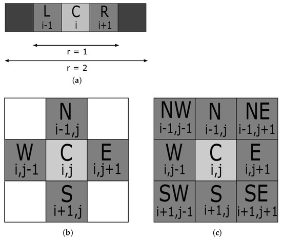
Figure 1.
(a) One−dimensional (1−D) CA with 5 cells, where C is the central cell, whose state is affected by its Left L and Right R neighbors, in range from it. (b) Von Neumann neighborhood configuration in 2-D CA. (c) Moore neighborhood configuration in 2-D CA.
In the case of two-dimensional CA (2-D CA), the most common neighborhood types are the von Neumann and Moore neighborhoods. The former includes the cell’s four adjacent neighbors (North N, South S, East E, West W), shown in gray in Figure 1b, while the latter includes, in addition to the von Neumann neighborhood, the cell’s four diagonal neighbors (Northeast , Northwest , Southeast , Southwest ), as shown in Figure 1c. Equations (3) and (4) express these relationships mathematically and show the interactions between the respective neighbors.
Every cell is initialized, and its state evolves synchronously in discrete time steps. Therefore, in every time step, all the cells update simultaneously their state. Calculating a cell’s new state depends on a rule f. This state update rule f takes into account several parameters, such as input from other cells, the cell’s neighbors as described in the previous paragraph; inputs from the environment as well as taking into consideration its own state, and depending on the relationships dictated among the neighboring cells by the rule, the new cell state is computed. As an example, we have Elementary CA (ECA) Rule 90, where each cell updates its state, taking into account the current state combination of its Right R and Left L neighbors as well as its current state ( cell C). The input combinations define the rule truth table, as shown in Table 1, and the central cell’s C next state can be computed. The notation chosen for ECA rules is based on Wolfram’s notation introduced in [53], where all transition rules f are encoded to numbers ranging from 0 to depending on the binary representation of the rule’s outcome set. As an example, in the case of Rule 90, the outcome set is , which translates to . The Boolean logic function describing the rule can be calculated, as shown in Equation (5), and its evolution is shown schematically in Figure 2a. In this case, the rule’s evolution is a repetitive pattern, as seen in Figure 2b, but there are also rules whose evolution indicates a random behavior.

Table 1.
Elementary CA Rule 90.

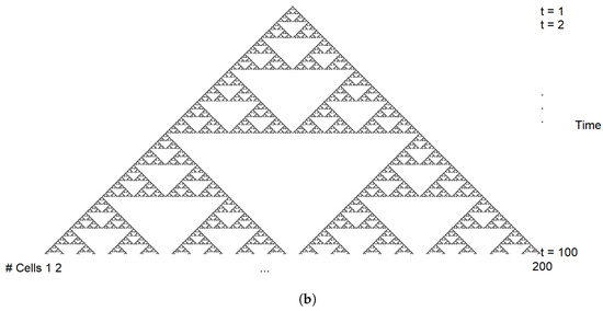
Figure 2.
(a) ECA Rule 90 for a 1-D CA consisting of 20 cells and 10 time steps of evolution. (b) Example of the time evolution of ECA Rule 90 for 200 cells and 100 time steps.
Lastly, what needs to be defined is how the boundary cells, which are missing some of their adjacent cells, are handled. There are multiple boundary conditions options available, but the most common ones are periodic, fixed, adiabatic, and mirrored, as shown in Figure 3. Taking as an example the case of ECA, where the two boundary cells, (), are both missing one adjacent cell, depending on the boundary conditions, Table 2 shows which cells affect the two boundary cells. The next state of the first cell is computed as a function of its current state , its Right R neighbor’s state , and its Left L neighbor’s state, considering 4 different cases for this neighbor, depending on the applied boundary conditions. Therefore, in the case of periodic boundary conditions, the last cell is used as the Left neighbor. Fixed boundary conditions translate as the use of a fixed value of either 0 or 1 as the missing neighboring cell, while adiabatic boundary conditions copy the cell’s under examination (here ) state to the missing neighbor’s state. Finally, if mirrored boundary conditions are selected, the Left neighbor’s value is selected to be the same as the Right neighbor’s, here equal to . Having explained the case for cell , the same rules can be applied to the last cell to compute the Right neighbor’s state that will be used in each case of different boundary conditions. For all other cells , where and , their next state is a function of their Right and Left neighbors, which can be summarized as follows, . These cases can be generalized for all N-dimensional CA grids.
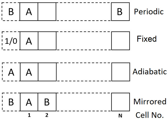
Figure 3.
Schematic describing the four types of boundary conditions.
Table 2.
Definitions for boundary conditions.
2.2. Memristor Devices and Models
2.2.1. Performance Characteristics and Functionality
The term was first introduced in 1971 by Leon Chua [18] and is a concatenation of the words “memory” and “resistor”. As suggested by its descriptive name, the memristor is a resistive device that exhibits memory properties. In 1976 [54], the memristor was included in a more generalized class of memristive systems. A pinched hysteresis loop on the plane is the hallmark of all memristive devices [55]. Nowadays, the term memristor is commonly used to refer to a class of two-terminal nonvolatile resistive switching nanodevices, whose resistive state can be modified.
It has been shown that a memristor can be programmed in a wide range of resistive states. However, for practical applications, it is important to be able to accurately program and read a number of distinct states, where . In the most simple case of binary memristive devices, they can be in one of two distinct states: the Low-Resistance State (LRS) and the High-Resistance State (HRS) . In the literature, memristive devices of multiple states can be found, such as the ones in [56,57,58], where the memristors can be accurately programmed to more than two distinct states. Each memristor can be characterized by its function, which defines the relationship between the voltage applied at its terminals and the current flowing through it. In the case of memristors with two stable distinct states, the memristor switches between high-resistance () and low-resistance () states. The transition from to is called the process, while the transition from to is called the process. For most applications, it is desired to have a high ratio, whereas a higher value is also desirable for lower power consumption.
During the last 15 years, memristive devices are being increasingly exploited for the design of circuits and systems both in academia but also in industry-related implementations. This exponential growth was triggered by a 2008 paper [17] where they connected the mathematical memristor framework with the fabrication of a nanoscale device. Evidence of memristive behavior had been presented before 2008, and other references also pre-existed in the literature such as the ones in [59,60,61,62]. In 2008, the authors of [63] acknowledged that their device described in [62] three years earlier was, in fact, a memristor. The main application of memristive devices has been their use as resistance switches for the design of non-volatile memories [64,65], attributed to their capability to maintain their resistive states without the requirement of frequent refreshing. Apart from that, memristive devices have been exploited for a plethora of applications, ranging from image processing applications such as in [66], where the authors present a reconfigurable memristor crossbar capable of convolutional image filtering implemented using hafnium oxide memristors, and in [67], where an image compression hardware accelerator is implemented using a memristor crossbar achieving a low-power and low-area solution. Memristors have also been identified as promising candidates to be used as building blocks of neural networks as in [68], where the memristors are used to store the synaptic weight and in [69] where an in-memory architecture for neural networks training is proposed. Additionally, memristive sensors have been fabricated capable of detecting cancer markers [70], while the author in [71] presents the rapid development of memristive sensors in the last 11 years. Finally, the authors in [72] describe the implementation of quantum computations using memristive grids.
There is a growing number of companies that, inspired by the promising characteristics of ReRAM technology, aim to manufacture and promote the use of Integrated Circuits (ICs) where memristive technologies are exploited. [73] is offering embedded solutions based on ReRAM technology for Internet of Things (IoT) applications, while [74] aims to commercialize the use of novel ReRAM devices on embedded memory, Edge Artificial Intelligence (Edge AI) and microcontrollers. [75] was established in 2018 and pursues the utilization of In-Memory Computing (IMC) technology for edge applications. and [76] have collaborated to develop a mass production process for next-generation ReRAM. Furthermore, companies such as [77], [78], [79], and [80] are also offering their products to customers. products span from discrete memristor devices to crossbar grids. Exploiting these products requires the use of peripheral circuitry for programming and sensing. In the case of , the company offers next-generation ReRAM, taking advantage of the technology’s high-performance prospect, reliability, low power consumption, and non-volatility characteristics. is currently offering its first 3D NAND memory called , a non-volatile memory capable of high-capacity and high-speed data storage developed using technology. is an array control system that allows conducting measurements and characterizing emerging ReRAM devices and crossbars offered by .
2.2.2. Device Models for Simulation
The research interest around memristors is growing rapidly, and the accurate simulation of the circuits under development makes it essential to provide researchers with the appropriate memristor models that describe the device’s behavior in good detail and in accordance with physical devices’ characteristics. A wide variety of models have been presented in the literature since the first model was presented in [17], where the memristor was modeled as a coupled variable resistor consisting of a doped and an undoped region whose width modification determined the memristor’s state. The two main categories of memristor models are behavioral and physics-based models. In the first case, the device’s behavior is described using appropriate mathematical relations. One such example of a behavioral model can be found in [81], where the memristor is considered to be a variable resistor. Depending on the materials used and the physical phenomena that govern the device’s functionality, there is an abundance of physics-based models also presented in the literature. In this case, the behavior of a fabricated memristive device is studied, and the model is developed. An example of this type of model is the Stanford-PKU ReRAM model [82], where the device’s conducting mechanism consists of the formation and rupture of a conductive filament. Next, three memristor models that have been extensively used in previous works will be discussed in more detail. These models have been selected for representing examples of the two different types of memristor models mentioned above (behavioral and physics-based models) that have been applied in various cases, as well as because they have been previously used in the applications reviewed in this work; therefore, understanding their characteristics is essential. It needs to be noted that the choice of the memristor model used in every application depends on the desirable characteristics of the designed circuit. Behavioral models provide a generalized option and can be used to attribute the behavior of memristive devices without the need to refer to a specific fabrication technology.
- A threshold-type behavioral memristor model
The model presented in [83] is a behavioral memristor model of a threshold-type voltage-controlled memristive device. The memristor’s switching is affected by the quantum tunneling distance modulation [84] used as the main electronic transport mechanism. The model is composed of an ohmic variable resistor R connected in series with a variable resistor . The model focuses on metal-oxide memristor devices; thus, R represents the resistance of the doped dioxide layer that has conductive properties, while represents the tunneling resistance of the undoped layer acting as a pure insulator. Given that , the model focuses mostly on . This resistance is affected by both the tunnel barrier width as well as the oxygen deficiencies transport resulting from the movement of the boundary that separates the two materials. Appropriately tuning the model’s parameters leads to the conclusion that the model can be fitted to numerous fabricated memristive devices while retaining the characteristic memristive fingerprints. In order to make it available for circuit designers, this model has also been implemented as a subcircuit in through a simple netlist consisting of existing electronic elements, as shown in Figure 4a, where the memristive device subcircuit consists of two current sources and an integrating capacitor. Handling the boundary conditions is realized using one more current source and direct current voltage sources connected in series with diodes. In Figure 4b, the model’s behavior is presented and specifically its I-V curve as well as the device’s memristance change in response to the applied voltage at its terminals (Figure 4c).
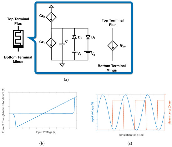
Figure 4.
(a) equivalent circuit implementing the memristor model in [83]. (b) I-V response. (c) Memristance update (orange) in response to the applied voltage (blue).
- Generalized Boundary Condition Model
The Generalized Boundary Condition Model (GBCM) [85] has been proposed as a generalization of the Boundary Condition Model (BCM) [86] in order to account for memristor properties not included in the BCM. More specifically, the GBCM is a mathematical memristor model developed to describe memristor dynamics such as the supra-threshold excitation property, which is a result of the filament formation and rupture and is the reason for the device’s bipolar resistance switching effect. This characteristic was not represented in the original BCM model. The equations describing the model’s behavior take inspiration from the original dopant drift model [17]. The memristor’s state is the variable used to describe the conductive part of the nanostructure, for example, the length of the -based layer in the case of titanium dioxide memristors [17,87] or the length of the conductive filament in the case of Conductive Bridge Random Access Memories (CB-RAM) [82,88].
A circuit realization of the GBCM model using the software, inspired by [89] was also presented and is shown in Figure 5. Modeling the memristor’s state required measuring the voltage across a capacitor C. Next, there is the series connection of two resistors, the linear resistor R and the non-linear, voltage-controlled one, . As the model’s mathematical description dictates, the boundary conditions of the model need to be set and this is achieved through the set of identical boundary cells. Each boundary cell is made up of two voltage-controlled switches whose functionality is to be activated/deactivated when the voltage across the capacitor reaches its bounds/surpasses the activation threshold. Furthermore, the activation cell consists of two voltage-controlled switches and two current controlled current sources. This configuration is used to model the memristor’s transition from the on to the off state and vice versa depending on the voltage applied to the memristor’s terminals.

Figure 5.
equivalent circuit of the GBCM model [85].
- Stanford-PKU ReRAM Model
In contrast to the previous two, the Stanford-PKU ReRAM model [82] is a physics-based memristor model. During the () process, the gap distance between the tip of the filament and the opposite electrode is decreasing (increasing) due to the oxygen-ion movement and vacancy generation and recombination events, resulting in the memristance decreasing (increasing) accordingly. This model’s behavior has been experimentally verified with various fabricated ReRAM devices and fitted to their physical characteristics. This model describes the behavior of a bipolar metal-oxide ReRAM device whose switching characteristics are attributed to the process of ion and vacancy migration within the device. As this is a complex process, developing a model that can appropriately describe the device’s characteristics required describing a more simplified process. Therefore, the device’s switching occurs due to the growth of a single conductive filament. In more detail, the device’s top layer () is called the top electrode (TE), and the bottom layer () is the bottom electrode (BE). When voltage is applied at these terminals, several parameters that act upon the device, such as the electric field, the oxygen-ion migration due to temperature change, and the temperature modification due to Joule heating, cause the formation of a conductive filament from the BE toward the TE, thus lowering the device’s resistance. Estimating the device’s resistance takes into consideration both the distance between the TE and the filament’s tip, called gap (g), as well as the filament’s radius, called width (w). The Stanford-PKU ReRAM model is -compatible and has been originally developed in . Its curve for 20 cycles is shown in Figure 6a, while the change in its (HRS) and (LRS) values, in response to the voltage applied to the device’s terminals, is illustrated in Figure 6b.
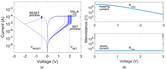
Figure 6.
(a) I−V simulation results for 20 cycles with the default variability applied, using a 400 s- period triangular voltage pulse from −3 V to 2.5 V and a 100 A compliance current for the SET process. (b) Boundary states and as a function of the applied voltage across the memristor (without variability), illustrating the conduction modes in HRS and LRS states. corresponds to and corresponds to . Adapted from [90].
3. Memristive Cellular Automata (MCA)
3.1. Theoretical Approach on MCA
In 2009, M. Itoh and L. Chua proposed a Memristor Cellular Automaton (MCA) for the first time [91]. An MCA is a rectangular array comprising identical memristor-based cells connected to each other via identical interconnections. Each cell consists of a passive memristive device and a switch, as shown in Figure 7a. The memristor model used in this work is an ideal, theoretical model whose memristance is a function of the charge q flowing through it and the current flow , defined as , whose response is shown in Figure 7b and can be tuned accordingly depending on the desired behavior by appropriately selecting the desired a and b values of the function as shown in Figure 7b.

Figure 7.
(a) Memristor CA cell, illustrating the memristor used to store the cell’s state and the current pulse generator (pink) that controls the switch to distinguish between the and the phases. (b) Selected memristance function.
A current pulse generator (shown in pink in Figure 7a) is used to control the switch, where a positive pulse turns on the switch, thus allowing the measurement of the memristance. When the current pulse is negative, the memristor discharges. Not applying negative pulses to the memristor results in its charge further increasing. The MCA’s time evolution is performed in discrete time steps, where each time step comprises two distinct phases: the phase and the phase. This switch allows either writing a new state to the memristor ( phase) or reading its state ( phase). The cell’s output is described by Equation (6).
where is the device’s memristance, and is the current pulse amplitude.
The above-described cell configuration was then used to perform logical operations. In this application each cell is independent, and changing its state depends on an input voltage-controlled current source. Choosing different functions to describe the memristance allows designing various logical operations such as , , and . The selected function for each case is shown in Table 3.
Table 3.
Memristance functions for various logical operations.
This proposed cell was used as the building block for the realization of a Memristor Cellular Automaton. As shown in Figure 8, this cell consists of the memristor cell described above , the current pulse generator that controls the switch, a signal generator that provides the positive and negative pulses that are used to charge and discharge the memristor, and voltage-controlled current sources (VCCS) acting as inputs to the cell.

Figure 8.
A Memristor Cellular Automaton cell consisting of a memristor cell as shown in Figure 7a, a current pulse generator (pink), a signal generator (purple), and a voltage-controlled current source (VCCS) denoted by a diamond-shape symbol (green). Neighboring signals correspond to incoming signals from other VCCS.
Connecting many of the above-described identical cells in an N-dimensional grid configuration, where , and appropriately selecting the memristor’s characteristics results in a Memristor Cellular Automaton that is capable of showcasing a wide variety of behaviors. The reprogrammability potential of memristors as well as their ability to maintain the resistive state they are programmed to, which can be exploited to store the CA’s state, contributed to its selection as the building block of the CA cell. Several applications have been selected to demonstrate the MCA’s functionality in [91]. First, the authors implemented the Elementary CA rule 126 by utilizing the appropriate memristance value and connecting MCA cells in a 1-D configuration. A more complex application includes the generation of the Sierpinski triangle, which requires the use of a four-state CA cell. Additional applications of this MCA also include the two-dimensional totalistic CA. In this case, every cell can be in one of two distinct states (0 or 1), and it has eight neighbors (Moore neighborhood) while also receiving feedback. Lastly, the proposed MCA was used to implement image processing algorithms such as horizontal hole and edge detection, erosion, dilation, Laplacian and sharpening filters, and noise removal. All the previously mentioned image processing operation tasks were examples presented in [91].
The dynamics of the MCA are described by the following Equation (7).
where is the memristance update function, y is the cell’s state (output), u are the external system inputs, T is the time period required for the system’s generation to be updated, is the charge accumulation in the memristor so far, and and are weight values passed on to the neighboring cells. These weights are the elements of two matrices.
3.2. Circuit Implementation of MCA
Inspired by the theoretical work of Itoh and Chua described above, the authors in [92] described in detail the Memristive Cellular Automata architecture where works like the ones presented in [93,94,95] were analyzed. In these works, the authors have presented several fields where MCAs have been successfully applied, such as shortest-path computing, sorting, and bin-packing problems. More specifically, in [94], the authors designed a two-dimensional memristor-based structurally dynamic CA, capable of detecting the nodes of a given mesh belonging to a shortest-path solution. The effectiveness of the CA-based computing system was evaluated both for single source-single destination and also for multiple destination scenarios of the problem. Most importantly, each cell contained a network of five memristors, which formed a “memristive fuse” configuration to disable further switching of input memristors once certain conditions have been met. Despite the fact that the switching of oxide memristors may yield large programming energy, since not all devices are required to switch in every cycle as well as taking advantage of the low voltage required to perform their switching, the system’s overall energy consumption will not constitute a problem. Additionally, memristive devices are characterized by their inherent stochasticity. The effect of this randomness in the device’s behavior has been examined in the case of Probabilistic Memristive Cellular Automata, which will be analyzed in this work. In cases where the memristor’s inherent variability is undesirable, measures can be taken toward minimizing its effect, such as using larger programming voltage values and times, so as to ensure that the desired switching will be achieved.
Later, the authors in [96] proposed a circuit-level approach of a one-dimensional MCA (1-D MCA) and later extended and modified their design to implement two-dimensional (2-D) applications as well [97,98]. As described in Section 2.1, in CA, the computation and storing of information is performed on the same physical unit. Therefore, storing each cell’s state is achieved using the memristor, while the computation is performed by a module. The memristor was selected to act as the storing element and switch its state among the and as it has low power consumption and will help maintain the overall system’s consumption low as it only requires switching among the two different states to achieve the desired outcome. Furthermore, memristive devices are small in size and can store the binary state necessary for the memristive CA evolution more efficiently compared to the conventional CMOS that would be required for the same process, while at the same time enabling in-memory computing. The selected memristor model in this case is no longer a theoretical model like the one used in [91] but it is a behavioral memristor model developed by Vourkas and Sirakoulis in [81], presented in more detail in Section 2.2.2. In the initial theoretical study in [91], depending on each application’s requirements, the authors used various memristance functions. Instead of describing the switching rate depending on the current passing through it, the majority of memristor models use voltage thresholds to describe the device’s behavior, where the switching rate depends on the applied voltage. Therefore, the circuit implementation of MCA requires the use of a memristor model that fulfills these requirements.
In this case, to fit to the required behavior, the Vourkas–Sirakoulis model was selected. The selection of a different model makes it necessary to appropriately modify the MCA cell in order to adjust the proposed circuit to the model’s requirements. These modifications include changing the connectivity of the switch that alternates between the and the phases, as in this case, the memristor model is voltage-controlled. Affecting a memristor’s state requires a voltage difference at its terminals whose value is high enough to exceed its voltage threshold and set or reset the memristor. On the other hand, sensing the memristor’s state without affecting it is done by applying a voltage of low enough value that is not capable of affecting its state but only reading it. Implementing these in the circuit requires grounding the memristor’s bottom terminal during the phase so that the voltage applied at its top terminal can affect its memristance when necessary, while reading it will connect its bottom terminal to the cell’s output in parallel to an RC delay circuit that will form a voltage divider. This was achieved using the switch as shown in Figure 9a. During its evolution, each cell of the MCA must receive a low-amplitude reading voltage pulse and also receive a resetting negative pulse to reset the memristor to its state so that it can be changed again depending on the rule, according to which writing voltage pulses will be applied to the cell when dictated by the rule. The reading pulse is only applied during the phase due to the grounding of the memristor afterward. An RC delay circuit is connected to the memristor’s bottom terminal, whose resistance and capacitance values were appropriately selected so as to maintain the output signal’s amplitude for a sufficient amount of time and be able to distribute it to the cell’s neighbors and affect their states. All the above as well as the signal used to initialize each cell’s state are global signals distributed to all the cells. Figure 9b demonstrates the cell’s output when its state is (red), (green) and the reading pulse duration (blue).

Figure 9.
(a) Schematic of the MCA cell’s circuit illustrating the memristor where the cell’s state is stored. Both multiplexers include the circuits that are controlled by the Control Signal, and distinguish among the and phases. (b) Cell’s output voltage in State 1 (red), State 0 (green), and applied reading pulse (blue).
3.2.1. 1-D Memristive Cellular Automata
The most simple and widely used form of 1-D CA is Elementary Cellular Automata (ECA). which were extensively described in Section 2.1. Therefore, in order to demonstrate their design’s functionality, the authors in [96] designed a 1-D MCA cell that is able to implement ECA rules. Taking inspiration from [91], this cell was used as a building block for a 1-D MCA configuration used as a pseudo-random number generator. Pseudo-random numbers provide the values that are necessary for processes that require randomness such as simulation methods (e.g., Monte Carlo) [99,100], electronic games [101], cryptography [102,103], etc.
Storing the cell’s state was described above and is composed of a memristor to store the cell’s state, a voltage-controlled switch to alternate between the phase and the phase, the RC delay circuit, and the required voltage pulse sources. Owing to the memristor’s reprogrammability feature utilizing appropriate voltage pulses, this device proves to be ideal to switch among the states of the CA as well as provide a storage device. Updating the cell’s state requires the circuit implementation of the rule. As this is an Elementary CA application, the computation of the next state will take into consideration only each cell’s two closest neighbors, its Left (L) and Right (R) neighboring cells, and it will also receive feedback (C). Every cell can be in one of two distinct states, namely 0 and 1. In Figure 9a, the circuit receives the three signals (), and depending on the selected transition rule f, these signals control voltage-controlled switches that compute the applied rule’s outcome. Therefore, if, according to the rule, the cell’s next state is 1, a voltage of high enough positive value will be applied to the memristor’s top terminal so as to set its state to . Otherwise, the complementary rule, which is also implemented in the block, will apply a negative voltage pulse to the memristor in order to reset its memristance to the state. As an example, the authors demonstrated the implementation of ECA Rule 126 as well as its complementary rule, as shown in Figure 10 described by the following Boolean functions:
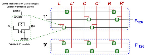
Figure 10.
Next-State Computation circuit for pseudo-random number generation for ECA Rule 126. The top circuit configuration is used to program logic ’1’, while the bottom circuit its complementary, ’0’. Every cell’s input controls a voltage-controlled switch that implements the desired rule.
In order to generate pseudo-random numbers, the authors were based on the ECA rules classification made by Wolfram in [104], who suggests that Rules 30 and 45 are the most suitable rules for pseudo-random number generation. Therefore, in the proposed circuit, based on the design strategy described for Rule 126, Rules 30 and 45, whose Boolean functions are shown in Equations (10) and (11), respectively, were combined and alternating every three time steps yielding a random enough sequence to be unpredictable, based on the evaluation performed using MATLAB©. To test the sequence’s randomness, the method selected [105] is called the Runs Test. Each run is defined as a non-stop series of increasing or decreasing values. The run’s length is equal to the number of these increasing or decreasing values. When the set of values comprises random data, then the probability that the value is followed by a larger or smaller value follows the binomial distribution. The results of the MCA’s evolution are shown in Figure 11a, while the generated numbers in format are shown in Figure 11b.
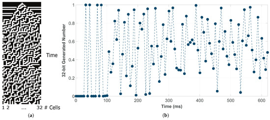
Figure 11.
(a) Proposed memristor-based CA evolution with two alternating rules every three time steps (Rule 30 and Rule 45) for periodic boundary conditions. (b) 32-bit generated pseudo-random numbers. Adapted from [96].
3.2.2. 2-D Memristive Cellular Automata
Extending the work presented in [96], the authors proposed two applications of 2-D MCA, using the above-described cell as a basis for their work. In more detail, the basic circuit used for each cell’s state storage remains the same in all cases. What needs to be adapted depending on the selected application is the circuit. This depends both on the update rule and on the number of neighboring connections each cell has.
- Epilepsy modeling using MCA
The first application that was presented was in [98], where the authors, based on work in [106], described the implementation of a 2-D MCA used to model normal and epileptiform brain activity. Epilepsy is a brain disorder whose characteristic is a temporary, sudden disruption of the brain’s normal function that can occur multiple times in one’s lifetime and is caused by a synchronized excitation of multiple neurons [107]. Several attempts have been made to model and detect epilepsy, among which are computational methods [108,109], artificial neural networks [110,111], and reservoir computing techniques [112]. The authors of [113] described the use of CA to model epilepsy propagation phenomena. Their proposed model consists of CA grids used to map the connectivity of brain neurons on a network of identical, interacting cells. As the purpose of this work was to demonstrate the interaction between a healthy and an epileptiform brain region, two CA grids are necessary, one that represents a healthy brain region and one that represents a brain region where epileptic activity can arise. The goal of this work was to investigate how the emergence of epileptic activity in one brain region can affect and spread to other regions. The neighboring connections in this case do not follow the typically chosen neighborhood types for 2-D CA, Moore and von Neumann as described in Section 2.1, but, in contrast, every cell can be affected by any other cell in its grid; therefore, longer distance connections are possible. Communication among the two grids is achieved by allowing only a small sub-grid of each CA to communicate with cells of the other grid.
As it is necessary for all CA, the rule needs to be specified. According to this rule, the block will be designed. The activation of a cell (transition from State 0 to State 1) can be caused by one of two reasons:
- The aggregated input signal the cell receives from all its neighbors exceeds a certain activation threshold.
- The cell receives an external, random excitation signal , which also exceeds a threshold (not necessarily of the same value as in case (1))
As previously mentioned, the number of neighbors is not fixed, and each cell has a variable amount T of connections labeled as to . During the healthy phase, all cells can have, at most, incoming signals. This number can be reduced to when an epileptic seizure occurs as the cells lose some of their connections during this phase. Therefore, for the neighboring connections, it is true that, .
One of the neurons’ characteristics that is taken into consideration in this work is the neuron’s refractory period. This refractory period consists of a certain amount of time during which a neuron will remain inactive and cannot be affected, regardless of the excitation it receives from its environment.
The circuit used to store the cell’s state remains the same as the one for the 1-D MCA case, shown in Figure 9a. However, the block needs to be modified and adjusted to the requirements of the specific application. In more detail, every cell will now receive input from more than two neighbors. These inputs will be averaged using an analog Millman adder [114], and the result will be compared with the pre-selected activation threshold of the switch mentioned above. If the result exceeds the threshold value, the switch is activated, and consequently, a write pulse is applied to the memristor driving it to the state. In the opposite case, the memristor remains unaffected. Implementing the external excitation of the cell requires one more voltage-controlled switch that controls the signal and is only activated when its threshold is exceeded (). If at least one of these two cases is met, then the positive voltage will be applied at the node. Resetting the memristor to is performed at every time step by applying a negative voltage to the memristor’s top terminal, at the beginning of the phase, before writing the new computed state. However, as shown in Figure 12a, the positive signal will affect the memristor only when is turned off. This switch is controlled by the cell’s feedback, and it ensures that the cell will only be activated two time steps after its last activation. This corresponds to the excitation and refractory times of real neurons. To control the number of time steps during which the cell remains inactive, a second delay circuit is necessary. When the cell’s output is 1, the switch controlled by the cell’s output will close, thus charging the module, and the switch will open, not allowing the signal to affect the memristor’s state.

Figure 12.
Next−State Computation circuits for (a) epileptic brain activity modeling and (b) Game of Life. In (a) VC switch stands for voltage-controlled switch. The Millman averaging configuration applies the average () of all inputs to the VC switch. delay is a parallel RC circuit. In (b), the comparator is implemented as shown in the dotted circuit, using 2 Operational Amplifiers.
To showcase the MCA’s functionality, the authors chose to simulate using Cadence PSPICE© software, two MCA grids, according to the aforementioned design characteristics. In both grids, each cell could have to neighboring connections, an amount chosen randomly for each cell. Achieving interconnectivity between the two grids was through the connection of some cells in the center, a sub-grid of each CA. All voltage-controlled thresholds were chosen to be equal to V. As shown in Figure 13a, when increased brain activity occurs in the pathogenic region (from time 2.5025 s to 3.7538 s), the healthy region is also affected, as shown in Figure 13b, resulting in the emergence of epileptic-like phenomena.

Figure 13.
Aggregate brain activity evolution in time for (a) the pathogenic and (b) the healthy brain region. Adapted from [98].
- Game of Life
One of the most well-known applications of 2-D CA is the Game of Life (GoL), proposed in 1970, by the mathematician John H. Conway and publicly appeared in Martin Gardner’s Scientific American column [115]. GoL is a zero-player game, meaning it does not require any user input, and it evolves autonomously over time. All that needs to be specified in every cell’s initial state as well as the rule. Although a variety of rules have been proposed and tested, the most widely used and interesting one is the one described by Equation (12), which can result in the generation of complex patterns and be used to imitate the functionality of a universal Turing machine.
Conway’s main idea when developing GoL was to observe a living organism’s (which corresponds to a CA cell) response to state changes of other organisms in its environment and how its state can be affected by them. Like all CA, GoL’s definition requires specifying the available set of states, state evolution rule, and neighborhood type. The most widely known GoL variation that Conway suggested is that of a system of dead or alive interacting organisms (cells). Therefore, a two-state CA, where logic 0 corresponds to dead and logic 1 corresponds to alive, is adequate to describe that. The cell states set can be described as . One more attribute that needs to be specified to complete the CA’s description is the cells’ connectivity. For the case of GoL, Conway chose a 2-D grid, where the connections between the cells were bidirectional, and the neighborhood type chosen is the Moore neighborhood, where, as described above, every cell is connected to its eight surrounding, closest neighboring cells. Computing the cell’s next state requires defining the evolution rule. Conway’s original idea included the requirements for a cell to survive, be born, and die. As seen in Equation (12), this rule dictates that when a cell is alive and it has two or three neighbors who are also alive, it will survive in the next generation (time step), . In case the cell is dead and exactly three of its neighbors are alive, the cell will be born. In all other cases, the cell will die in the next time step, as a result either of overcrowding or loneliness. This rule can be described as , where B stands for Birth and S for survival.
In [97], the authors propose a circuit implementation of an MCA cell that can simulate the behavior of GoL. As described in the previous cases, storing the cell’s state requires a memristor as well as a voltage-controlled switch that can alternate among the two phases of each time step, the phase and the phase. Apart from this, implementing the rule requires designing the circuit for this specific case. In order to realize the rule presented above, it is necessary to add all the input signals that a cell receives. This was realized using an analog Millman adder circuit which acts as an averager [114], like the one used in the previous application. Therefore, the voltage at node is equal to the weighted average value of all the inputs. What needs to be noted is that the cell also receives feedback, necessary for the specific rule. All input signals are connected to the common node through equal-valued resistors. This is not the case for the feedback signal, for which a resistor equal to 2 × the resistor mentioned before, was selected. This selection was made because, in contrast to the neighbors, whose only total amount of alive cells affects the rule’s outcome, the feedback’s state affects the rule’s outcome. Therefore, when a neighbor’s signal is 1, it counts as 1 for the computation of the average, while when the feedback signal is 1, the different resistance value means that it will only contribute as of the rest. So, the B3/S23 rule is now translated to a cell remaining alive only when the averager output is equal to or greater than 2.5 and equal to or less than 3.5. The value computed through the Millman adder is passed as an input to a voltage window comparator, as shown in Figure 12b, that will perform the necessary comparisons and will apply a positive voltage pulse to the memristor’s top terminal only when and set its state to . In all other cases, the applied voltage has negative amplitude, used as a reset voltage pulse, to reset the memristance to the state. The voltage window comparator used in this work was designed as suggested in [116], using two operational amplifiers (op-amps).
In the voltage comparator, the first op-amp has an inverting input terminal connected to the higher voltage value limit (0.35 V), while the second op-amp has the lower voltage limit (0.25 V) connected at its non-inverting input. The input voltage value that is to be compared is given as input to the common node where the non-inverting input of the first op-amp and the inverting input of the second op-amp are connected. When the algebraic difference between the input signal and the set-point voltage changes polarity, the set-point voltage is chosen for the set-point level at which the linear output of the first operational amplifier crosses from one polarity to another. As a result, as the input signal decreases to the point where the output of the first operational amplifier reverses polarity, the output of the second operational amplifier switches from the first to the second level and remains at the second level until the input signal drives the output of the first operational amplifier to the point where it exceeds the window-width voltage. It then returns to the first level and stays there until the input signal increases enough for the output of the first operational amplifier to fall below the window-width voltage. Since the op-amps operate within their linear region and the input voltage is never equal to the comparator’s supply voltage, non-linearity effects that emerge at this region of the comparator’s functionality have not been of concern. In comparators, the transition from one state to another should ideally be instant; nonetheless, switching from one state to another will take some time. At the transitions, slanted edges can be seen. These transitions are more evident at higher frequencies, even higher than the period of the input signal itself. As a result, the comparator’s operating frequency has an upper limit. The maximum operating frequency is determined by the op-amp’s slew rate. The greater the slew rate, the greater the operating frequency. Because op-amps are used in comparator applications in open loop mode, frequency compensation is not necessary. In comparator applications, uncompensated op-amps are recommended. The two diodes split the outputs so that if either goes low, the op-amp turns on the transistor. The circuit assumes a conventional operational amplifier output; however, a comparator’s output structure may be completely different.
The MCA was designed and simulated in Cadence PSPICE© environment, and two different grids are presented to showcase the designed circuit’s functionality. Specifically, a and a grid, with periodic boundary conditions were initialized with the initial state shown in Figure 14a,f, respectively, while their time evolution for 4 more time steps is shown in the following sub-figures.
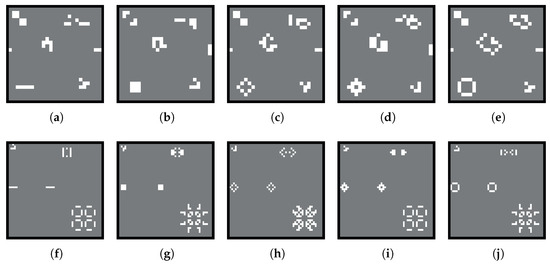
Figure 14.
Game of Life evolution in a (top a–e) and in a (bottom f–j) memristive CA cell grid. Gray cells correspond to State 0 (dead) and white ones to State 1 (alive). Adapted from [97].
4. Memristor Cellular Automata for Image Processing Applications
The work of Itoh and Chua inspired the authors of [117,118] to propose a Memristor Cellular Automaton where the Belief Propagation Algorithm (BPI) was chosen as the state evolution rule. The memristor model used in this case is a mathematical implementation originally presented by Ascoli et al. in [85] and analyzed in Section 2.2.2. In this work, the authors proposed a memristive CA that is capable of performing complex operations, in analogy to the one presented in [119].
The BPI is applied on a layer of cells, used as synapses, where each synapse returns a binary value. This binary value is the output generated based on the selected rule as well as the binary input pattern. Each cell has a memristance value , normalized in the range , where corresponds to and corresponds to 1. These memristance values correspond to synaptic weight values based on Equation (13).
where
Considering a CA grid consisting of N cells, a threshold parameter was set, where is the set of binary input patterns, and is the desired output for each input pattern and the stability parameter , which equals to:
Considering that, the state update rule can be defined as follows:
- if ,
- if ,
- with probability
- if ,
- else,
In this work, a two-state CA was selected and calculating the evolution dynamics of the cells requires making an analogy between Equation (7) and the CA designed using the BPI as described with the previous equations. Therefore, the cells’ evolution dynamics can be described as:
This system’s performance was evaluated in an image processing application that involves the detection of wounds in digital pictures for the demonstration of an improved and more efficient telediagnostic system. Traditional methods used for ulcer detection and evaluation of its size and severity mainly involve manual approaches performed by physicians and require direct contact with the wound, making the decision process inaccurate, costly, and increasing the variability and the possibility of human error. Novel digital methods have also been developed but can be affected by subjective interpretation and the environment. Therefore, the authors are tackling the issue by developing the presented BPI-CA system, which is able to detect wound contours with high precision. Testing the proposed BPI-CA was performed on RGB images, where the authors implemented the detection of specific color patterns. Three memristor-composed matrices, whose size is equal to the size of the image are processed, and a results matrix is generated after applying the BPI-CA. The selected images depicted cutaneous ulcers, whose color combinations are different from the background and allow the object’s identification, by taking the three separate color channels (red R, green G, and blue B) of an image and analyzing them. In more detail, each image pixel corresponds to a CA cell, and the neighborhood connections are based on the spatial relationship of the pixels. In a compact form, the state evolution rule for wound detection can be described in the following Table 4. The algorithm iterates across the image, processing all the pixels in parallel, and outputs a matrix containing the results.
Table 4.
BPI-CA color detection rule.
5. Memristive Probabilistic Cellular Automata
One of the characteristics of fabricated memristive devices is their inherent variability. During the set and reset process, real memristive devices do not always behave in the exact same way, as the formation and rupture of the conductive filament is an inherently random process. This leads to a probabilistic switching behavior, which is evident both spatially (device-to-device variations) as well as temporally (cycle-to-cycle variations). As a result, the memristor’s switching can be described by a Poisson distribution, where the switching probability is equal to , where is the characteristic switching time, while is an infinitesimal time interval. The parameter is exponentially dependent on the voltage applied at the memristor’s terminals, allowing, therefore, to appropriately adjust the device’s switching probability depending on the applied voltage pulse’s amplitude and width.
In [120], Ntinas et al. describe the use of a memristor with this behavior as a controllable circuit element for the design of a 1-D CA system capable of implementing Wolfram’s ECA rules, as they were previously described in Section 2.1. In all the cases described before, CA were deterministic in the sense that when the system receives the same input, the same rule will always produce the same outputs/next states. In this work, the authors introduce the concept of Probabilistic Cellular Automata (PCA), also known as locally interacting Markov chains [121,122], where the state update is governed by a probabilistic rule that dictates the probability, that given an input pattern at time t, the central cell will transition to each possible next state at time or not. As described above, in ECA, the Next-State Computation depends on the cell’s Left and Right neighbors as well as feedback, while the probabilistic rule describes the state update seen in Table 5, where and are the next states in these two cases that are determined probabilistically. A probabilistic ECA rule can also be decomposed into four deterministic rules , where each rule is governed by a probability .
Table 5.
Conditional probabilities table.
As described in Section 3.2, a memristor is used to store the cell’s state along with the necessary switches and voltage sources to program it. The rule’s probabilistic transitions are realized through the device’s probabilistic switching characteristics. The memristor’s switching probabilities depend on the programming voltage applied to it during the phase and, specifically, the pulse’s duration as well as its amplitude during , , and , . The memristor’s switching probability is equal to and , respectively. The circuit-level design in this case is shown in Figure 15.

Figure 15.
Circuit-level illustration of a MemPCA cell. First multiplexer is used to select the or process, while the other two include the circuits that are controlled by the Read/Write Control Signal and distinguish among the Reading and Writing phases.
Evaluation of the proposed system was performed by measuring the system’s entropy as a means to investigate the quality of the randomness that emerges from this MemPCA approach. A system’s entropy is often used as a measure of its randomness, and given a signal S with possible levels for a 1-D CA consisting of an array of cells , it can be calculated according to Equation (17).
Considering a MemPCA with , the generation of numbers was evaluated for time steps to test their randomness. The system’s stochasticity was measured for rule 110 for various values of failure probability of the memristor’s switching which is defined as . Testing several ECA rules demonstrated that the majority of achieve low entropy values while certain show the maximum entropy, both for the probabilistic as well as the deterministic case.
A novel hardware realization of memristor-based CA, which incorporates a combination of CMOS and memristor circuits, where memristor devices are integrated into both the state and rule modules, has been shown in [123]. By leveraging memristors as an entropy source in each CA cell, the proposed implementation achieves enhanced operational speed and reduced area requirements. The functionality of the proposed MemCA approach is demonstrated through deterministic and probabilistic operations, which can be externally adjusted by modifying the programming voltage amplitude, without necessitating any changes to the design. Moreover, this design includes a versatile rule module implementation, enabling spatial and temporal rule variations.
6. Memristive Excitable Cellular Automata
Research on Memristive Cellular Automata also includes the 2011 paper by A. Adamatzky and L. Chua, who proposed a memristive excitable cellular automaton [124]. In contrast to all the above-described works, which were all based on [106], and in which the proposed CA cell is made up of memristors as the main storage device, the memristive excitable CA presented in [124] are not CA in which the memristive properties are being exploited but rather have the ability to imitate memristive behavior.
6.1. Memristive Automaton
A memristive automaton is defined as a type of excitable CA whose characteristic is that when a cell is in the excited state, and another one is in the refractory state, links between them can be added or removed. The CA used in this case consists of an orthogonal grid of cells, each of which has three states, and the neighborhood type is the Moore. The three distinct states are the resting (o), excited (+), and refractory (−) states. The links connecting two cells x and y, denoted as , can be in one of two states: 0, which corresponds to non-conductive link, or high-resistance, and 1, which corresponds to a conductive link or low resistance. The link states can be updated depending on the states of the cells that are connected through them. Particularly, only non-resting cells will be taken into account, and considering that there cannot be any current flow between cells that are in the same state, it is considered that cells in the same state do not contribute to the link connectivity. The link state update rule is summarized in Equation (18).
where and . Therefore, two different types of automata can be defined, and .
As far as the resting cells are concerned, excitation occurs depending on the total sum of its excited neighbors. Calculating this sum can be performed in two different ways.
where if and otherwise.
Taking this into account, two different automata cases can be defined.
- , where a resting cell will be excited when .
- , where a resting cell will be excited when or .
6.2. Experimental Procedures
Testing the proposed memristive CA was realized using a , where , grid of identical cells. The boundary conditions chosen are non-periodic absorbing and the two different cases for the link conductivity were assumed. More specifically,
- , where all links are initialized to the conductive state, .
- , where all links are initialized to the non-conductive state, .
Initially, only the cells that belong to the area in the D radius, which is equal to from the central cell (), can be in the excited state (+). D-simulation consists of assigning the excited state to a cell within that radius with a probability equal to . When performing pointwise simulation, in the case of CA, a single cell needs to be in the excited state initially, while in CA, the excitation of a couple of cells is necessary for the initialization, allowing for the propagation to commence. As seen in Figure 16 and Figure 17, a CA leads to a persistent excitation of the cells, while a CA results in a resting state. The omni-directional propagation of the wave away from the center cell leads to a classical excitation wave front. In the case of CA, links are made non-conductive during the wave’s forward propagation, while in , the links associated with back propagation are made non-conductive. As an example, the wave propagation for a will be described, as shown in Figure 18.
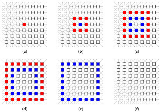
Figure 16.
(a) Excitation and link dynamics for a automaton for 6 time steps. Red squares correspond to excited cells (+), while blue correspond to refractory cells (−), and resting cells are left blank. An arrow connecting two cells means an active link between them, . Initial state in (a) and its evolution in (b–f) for each time step.
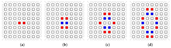
Figure 17.
Excitation and link dynamics for a automaton for 4 time steps. An arrow connecting two cells means an active link between them, . Initial state in (a) and its evolution in (b–d) for each time step.
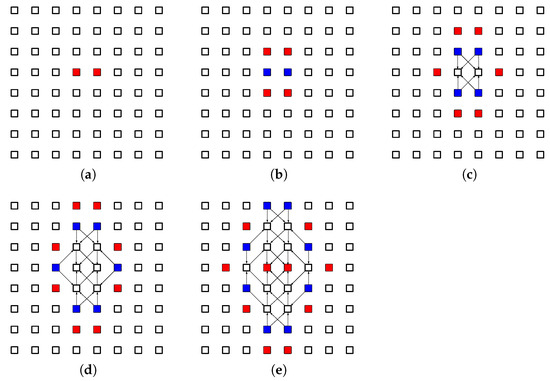
Figure 18.
(a) Excitation and link dynamics for a automaton for 5 time steps, -start. An arrow connecting two cells means an active link between them, . Initial state in (a) and its evolution in (b–e).
As shown in Figure 18a, the initially excited cells are two neighboring cells, on the same row. Based on Condition 2, where it is required that , and the north and south neighbors of both cells will be excited (Figure 18b). The excitation will then propagate north and south again and also east and west, as seen in Figure 18c. Next, the excitation wave will propagate again in the four directions, while the initially perturbed cells return to the resting state, as seen in Figure 18d. This pattern will eventually fill the CA grid (Figure 18e).
6.3. Distinguished Observations
6.3.1. Oscillating Localizations
Memristive excitable CA have also been used to observe the propagation of oscillations. There are two very common types of oscillations observed, namely the and types. In the first case, the minimal initial configuration consists of two cells, one in the excited and one in the refractory state, and 12 steps are required for a complete oscillation, while in the case of , two cells are also the minimum, but a larger number of steps, 26, is necessary.
6.3.2. Dynamics of Excitation on Interfaces
The excitation of a automaton leads to localizations that propagate in the boundary of ordered and disordered conductivity domains. Simulations demonstrated that the automaton becomes separated into two domains, where one is in the disordered state within the boundaries of D, while the other one is characterized by an ordered configuration of links. Worms of disordered excitation are created in the boundary between these two domains.
6.3.3. Building Conductive Pathways
Lastly, collisions occurring between traveling excitations in initially non-conductive mediums can result in building information transmission pathways. When two localizations are traveling in a automaton, under initial conditions, the collision between their propagating waves will be elastic and further particles will be formed.
7. Concluding Remarks and Discussion
This paper reviewed the most recent research efforts focusing on the design of Memristive Cellular Automata-based computing systems. Given the advantageous performance characteristics of resistive switching devices (memristors), exploiting their capability to enable storing and processing of information within the same physical units allows the development of novel and enhanced nanoelectronic circuits, which incorporate this new type of circuit elements. In this direction, Cellular Automata (CA) grids have been explored as a promising parallel computing platform for hardware-based solutions to several problems. Inspired by the behavior of the biological brain, Cellular Automata are models that incorporate the idea of storing and processing of information in the same unit, which happens to be the CA cell, and thus eliminate the need for data transfer. This idea motivated researchers to combine the architecture of CA with memristive devices and explore the performance and application prospects of such novel circuits and systems.
The basic theoretical approach was initially presented by Itoh and Chua, and this work inspired later more researchers to propose interesting realizations for Memristive Cellular Automata and corresponding circuit topologies. Apart from the theoretical approaches found in the literature, several circuit-level designs have been also presented. It becomes obvious from recent advances in the field that research efforts are being placed toward the implementation of a generalized realization of Memristive Cellular Automata, suitable for application in various problems of similar characteristics. In this direction, this review paper extensively discussed the existing literature on MCA and applications. The 1-D and 2-D implementations of CA carrying out image processing tasks and also other popular applications were initially described to showcase the architecture’s robustness. Next, the paper reviewed a specific CA variation, i.e., the Probabilistic CA, which can be implemented using memristive devices. The latter provide evidence of the ever-increasing area of applications that can be benefited from the exploitation of MCA. Lastly, a different approach to CA was pursued, i.e., the Memristive Excitable Cellular Automata-based systems, where the CA architecture was proven capable of imitating the memristive behavior.
Possible simplifications for the discussed systems are possible, concerning the design of the evolution rule. Moreover, designing appropriately any of the proposed systems in a way that allows the utilization of any memristor model type in simulations (thus the application to be functional with practically any type of real devices) is among the most important challenges to overcome toward a CA system architecture capable of adapting to various applications. Everything considered, through the comprehensive analyses presented in this paper, we conclude that the concept of “Memristive Cellular Automata” is a challenging yet very promising direction for the development of novel, beyond von Neumann parallel computing circuits and systems.
Author Contributions
Conceptualization, R.-E.K., I.-A.F., V.N., I.V., A.A. and G.C.S.; resources, R.-E.K., I.-A.F., V.N., I.V., A.A. and G.C.S.; data curation, R.-E.K., I.-A.F., V.N., I.V., A.A. and G.C.S.; writing—original draft preparation, R.-E.K., I.-A.F., V.N., I.V., A.A. and G.C.S.; writing—review and editing, R.-E.K., I.-A.F., V.N., I.V., A.A. and G.C.S.; visualization, R.-E.K., I.-A.F., V.N., I.V., A.A. and G.C.S.; supervision, I.V. and G.C.S.; project administration, G.C.S.; funding acquisition, R.-E.K. and I.V. All authors have read and agreed to the published version of the manuscript.
Funding
The research work of Rafailia-Eleni Karamani was supported by the Hellenic Foundation for Research and Innovation (HFRI) under the HFRI PhD Fellowship grant (Fellowship Number: 1333), while the research work of Ioannis Vourkas by the Chilean government under grants FONDECYT Regular No. 1221747 and ANID-Basal FB0008.
Data Availability Statement
Data is not available for privacy reasons.
Conflicts of Interest
The authors declare no conflict of interest.
References
- Bardeen, J.; Brattain, W.H. The transistor, a semi-conductor triode. Phys. Rev. 1948, 74, 230. [Google Scholar] [CrossRef]
- Shalf, J. The future of computing beyond Moore’s law. Philos. Trans. R. Soc. A 2020, 378, 20190061. [Google Scholar] [CrossRef]
- Esser, S.K.; Merolla, P.A.; Arthur, J.V.; Cassidy, A.S.; Appuswamy, R.; Andreopoulos, A.; Berg, D.J.; McKinstry, J.L.; Melano, T.; Barch, D.R.; et al. Convolutional networks for fast, energy-efficient neuromorphic computing. Proc. Natl. Acad. Sci. USA 2016, 113, 11441–11446. [Google Scholar] [CrossRef]
- Schuman, C.D.; Potok, T.E.; Patton, R.M.; Birdwell, J.D.; Dean, M.E.; Rose, G.S.; Plank, J.S. A survey of neuromorphic computing and neural networks in hardware. arXiv 2017, arXiv:1705.06963. [Google Scholar]
- van De Burgt, Y.; Melianas, A.; Keene, S.T.; Malliaras, G.; Salleo, A. Organic electronics for neuromorphic computing. Nat. Electron. 2018, 1, 386–397. [Google Scholar] [CrossRef]
- Torrejon, J.; Riou, M.; Araujo, F.A.; Tsunegi, S.; Khalsa, G.; Querlioz, D.; Bortolotti, P.; Cros, V.; Yakushiji, K.; Fukushima, A.; et al. Neuromorphic computing with nanoscale spintronic oscillators. Nature 2017, 547, 428–431. [Google Scholar] [CrossRef] [PubMed]
- Burr, G.W.; Shelby, R.M.; Sebastian, A.; Kim, S.; Kim, S.; Sidler, S.; Virwani, K.; Ishii, M.; Narayanan, P.; Fumarola, A.; et al. Neuromorphic computing using non-volatile memory. Adv. Phys. X 2017, 2, 89–124. [Google Scholar] [CrossRef]
- Kumar, S.; Williams, R.S.; Wang, Z. Third-order nanocircuit elements for neuromorphic engineering. Nature 2020, 585, 518–523. [Google Scholar] [CrossRef]
- Dutta, S.; Khanna, A.; Assoa, A.; Paik, H.; Schlom, D.G.; Toroczkai, Z.; Raychowdhury, A.; Datta, S. An Ising Hamiltonian solver based on coupled stochastic phase-transition nano-oscillators. Nat. Electron. 2021, 4, 502–512. [Google Scholar] [CrossRef]
- Wang, S.; Li, Y.; Wang, D.; Zhang, W.; Chen, X.; Dong, D.; Wang, S.; Zhang, X.; Lin, P.; Gallicchio, C.; et al. Echo state graph neural networks with analogue random resistive memory arrays. Nat. Mach. Intell. 2023, 5, 104–113. [Google Scholar] [CrossRef]
- Gibson, M.J.; Keedwell, E.C.; Savić, D.A. An investigation of the efficient implementation of cellular automata on multi-core CPU and GPU hardware. J. Parallel Distrib. Comput. 2015, 77, 11–25. [Google Scholar] [CrossRef]
- Bakhteri, R.; Cheng, J.; Semmelhack, A. Design and Implementation of Cellular Automata on FPGA for Hardware Acceleration. Procedia Comput. Sci. 2020, 171, 1999–2007. [Google Scholar] [CrossRef]
- Halbach, M.; Hoffmann, R. Implementing cellular automata in FPGA logic. In Proceedings of the 18th International Parallel and Distributed Processing Symposium, Santa Fe, NM, USA, 26–30 April 2004; IEEE: Pitcataway, NJ, USA, 2004; p. 258. [Google Scholar]
- Moore, J.H.; Hahn, L.W. Cellular automata and genetic algorithms for parallel problem solving in human genetics. In Proceedings of the International Conference on Parallel Problem Solving from Nature; Springer: Berlin/Heidelberg, Germany, 2002; pp. 821–830. [Google Scholar]
- Santé, I.; García, A.M.; Miranda, D.; Crecente, R. Cellular automata models for the simulation of real-world urban processes: A review and analysis. Landsc. Urban Plan. 2010, 96, 108–122. [Google Scholar] [CrossRef]
- Margolus, N.; Toffoli, T. Cellular automata machines. In Lattice Gas Methods for Partial Differential Equations; CRC Press: Boca Raton, FL, USA, 2019; pp. 219–250. [Google Scholar]
- Strukov, D.B.; Snider, G.S.; Stewart, D.R.; Williams, R.S. The missing memristor found. Nature 2008, 453, 80–83. [Google Scholar] [CrossRef]
- Chua, L. Memristor-the missing circuit element. IEEE Trans. Circuit Theory 1971, 18, 507–519. [Google Scholar] [CrossRef]
- Fox, G.C.; Williams, R.D.; Messina, P.C. Parallel Computing Works! Elsevier: Amsterdam, The Netherlands, 2014. [Google Scholar]
- Scott, L.R.; Clark, T.; Bagheri, B. Scientific Parallel Computing; Princeton University Press: Princeton, NJ, USA, 2021. [Google Scholar]
- Ulam, S.M. Scottish Book: A LASL Monograph. In Collection of Problems of Interest in Late 1930’s; Los Alamos National Lab.: Los Alamos, NM, USA, 1977. [Google Scholar] [CrossRef]
- Von Neumann, J. The General and Logical Theory of Automata; John Wiley and Sons: Hoboken, NJ, USA, 1963; Volume 5. [Google Scholar]
- Neumann, J.; Burks, A.W. Theory of Self-Reproducing Automata; University of Illinois Press Urbana: Champaign, IL, USA, 1966; Volume 1102024. [Google Scholar]
- Wolfram, S. Mathematica: A System for Doing Mathematics by Computer; Addison Wesley Longman Publishing Co., Inc.: Boston, MA, USA, 1991. [Google Scholar]
- Wolfram, S. A New Kind of Science; Wolfram Media: Champaign, IL, USA, 2002; Volume 5. [Google Scholar]
- Wolfram, S. Cellular automata as models of complexity. Nature 1984, 311, 419–424. [Google Scholar] [CrossRef]
- Kier, L.B.; Seybold, P.G.; Cheng, C.K. Modeling Chemical Systems Using Cellular Automata; Springer Science & Business Media: Berlin/Heidelberg, Germany, 2005. [Google Scholar]
- Kansal, A.R.; Torquato, S.; Harsh Iv, G.; Chiocca, E.; Deisboeck, T. Simulated brain tumor growth dynamics using a three-dimensional cellular automaton. J. Theor. Biol. 2000, 203, 367–382. [Google Scholar] [CrossRef]
- Zhang, Y.; Yang, Z.; Sun, Z. A dynamic estimation method for aircraft emergency evacuation based on cellular automata. Adv. Mech. Eng. 2019, 11, 1687814019825702. [Google Scholar] [CrossRef]
- Giitsidis, T.; Dourvas, N.I.; Sirakoulis, G.C. Parallel implementation of aircraft disembarking and emergency evacuation based on cellular automata. Int. J. High Perform. Comput. Appl. 2017, 31, 134–151. [Google Scholar] [CrossRef]
- Spartalis, E.; Georgoudas, I.G.; Sirakoulis, G.C. Ca crowd modeling for a retirement house evacuation with guidance. In Proceedings of the International Conference on Cellular Automata, Krakow, Poland, 22–25 September 2014; Springer: Berlin/Heidelberg, Germany, 2014; pp. 481–491. [Google Scholar]
- Georgoudas, I.G.; Kyriakos, P.; Sirakoulis, G.C.; Andreadis, I.T. An FPGA implemented cellular automaton crowd evacuation model inspired by the electrostatic-induced potential fields. Microprocess. Microsyst. 2010, 34, 285–300. [Google Scholar] [CrossRef]
- Koumis, I.; Georgoudas, I.G.; Trunfio, G.A.; Wąs, J.; Sirakoulis, G.C. A GPU implemented 3f cellular automata-based model for a 2D evacuation simulation pattern. In Proceedings of the 2017 25th Euromicro International Conference on Parallel, Distributed and Network-Based Processing (PDP), St. Petersburg, Russia, 6–8 March 2017; IEEE: Pitcataway, NJ, USA, 2017; pp. 497–504. [Google Scholar]
- Tourtounis, D.; Mitianoudis, N.; Sirakoulis, G.C. Salt-n-pepper noise filtering using cellular automata. arXiv 2017, arXiv:1708.05019. [Google Scholar]
- Rosin, P.L. Image processing using 3-state cellular automata. Comput. Vis. Image Underst. 2010, 114, 790–802. [Google Scholar] [CrossRef]
- Vezhnevets, V.; Konouchine, V. GrowCut: Interactive multi-label ND image segmentation by cellular automata. In Proceedings of Graphicon; Citeseer: State College, PA, USA, 2005; Volume 1, pp. 150–156. [Google Scholar]
- Hernández, G.; Herrmann, H.J. Cellular automata for elementary image enhancement. Graph. Model. Image Process. 1996, 58, 82–89. [Google Scholar] [CrossRef]
- Roy, S.; Shrivastava, M.; Rawat, U.; Pandey, C.V.; Nayak, S.K. IESCA: An efficient image encryption scheme using 2-D cellular automata. J. Inf. Secur. Appl. 2021, 61, 102919. [Google Scholar] [CrossRef]
- Alexan, W.; ElBeltagy, M.; Aboshousha, A. RGB Image Encryption through Cellular Automata, S-Box and the Lorenz System. Symmetry 2022, 14, 443. [Google Scholar] [CrossRef]
- Katis, I.; Sirakoulis, G.C. Cellular automata on FPGAs for image processing. In Proceedings of the 2012 16th Panhellenic Conference on Informatics, Piraeus, Greece, 5–7 October 2012; IEEE: Pitcataway, NJ, USA, 2012; pp. 308–313. [Google Scholar]
- Zhao, Y.; Billings, S.A.; Routh, A.F. Identification of the Belousov–Zhabotinskii reaction using cellular automata models. Int. J. Bifurc. Chaos 2007, 17, 1687–1701. [Google Scholar] [CrossRef]
- Dourvas, N.I.; Sirakoulis, G.C.; Adamatzky, A. Cellular automaton Belousov–Zhabotinsky model for binary full adder. Int. J. Bifurc. Chaos 2017, 27, 1750089. [Google Scholar] [CrossRef]
- Dai, J.; Zhai, C.; Ai, J.; Ma, J.; Wang, J.; Sun, W. Modeling the spread of epidemics based on cellular automata. Processes 2021, 9, 55. [Google Scholar] [CrossRef]
- Sirakoulis, G.C.; Karafyllidis, I.; Thanailakis, A. A cellular automaton model for the effects of population movement and vaccination on epidemic propagation. Ecol. Model. 2000, 133, 209–223. [Google Scholar] [CrossRef]
- Pokkuluri, K.S.; Nedunuri, S.U.D. A novel cellular automata classifier for covid-19 prediction. J. Health Sci. 2020, 10, 34–38. [Google Scholar] [CrossRef]
- Schimit, P.H. A model based on cellular automata to estimate the social isolation impact on COVID-19 spreading in Brazil. Comput. Methods Programs Biomed. 2021, 200, 105832. [Google Scholar] [CrossRef]
- Louis, P.Y.; Nardi, F.R. Probabilistic Cellular Automata: Theory, Applications and Future Perspectives; Springer: Berlin/Heidelberg, Germany, 2018; Volume 27. [Google Scholar]
- Ghosh, S.; Bhattacharya, S. A data-driven understanding of COVID-19 dynamics using sequential genetic algorithm based probabilistic cellular automata. Appl. Soft Comput. 2020, 96, 106692. [Google Scholar] [CrossRef]
- del Rey, A.M. A computer virus spread model based on cellular automata on graphs. In Proceedings of the International Work-Conference on Artificial Neural Networks, Salamanca, Spain, 10–12 June 2009; Springer: Berlin/Heidelberg, Germany, 2009; pp. 503–506. [Google Scholar]
- Schneckenreither, G.; Popper, N.; Zauner, G.; Breitenecker, F. Modelling SIR-type epidemics by ODEs, PDEs, difference equations and cellular automata–A comparative study. Simul. Model. Pract. Theory 2008, 16, 1014–1023. [Google Scholar] [CrossRef]
- Almeida, R.M.; Macau, E.E. Stochastic cellular automata model for wildland fire spread dynamics. Proc. J. Phys. Conf. Ser. 2011, 285, 012038. [Google Scholar] [CrossRef]
- Bartolozzi, M.; Thomas, A.W. Stochastic cellular automata model for stock market dynamics. Phys. Rev. E 2004, 69, 046112. [Google Scholar] [CrossRef] [PubMed]
- Wolfram, S. Statistical mechanics of cellular automata. Rev. Mod. Phys. 1983, 55, 601. [Google Scholar] [CrossRef]
- Chua, L.O.; Kang, S.M. Memristive devices and systems. Proc. IEEE 1976, 64, 209–223. [Google Scholar] [CrossRef]
- Chua, L. If it’s pinched it’sa memristor. Semicond. Sci. Technol. 2014, 29, 104001. [Google Scholar] [CrossRef]
- Stathopoulos, S.; Khiat, A.; Trapatseli, M.; Cortese, S.; Serb, A.; Valov, I.; Prodromakis, T. Multibit memory operation of metal-oxide bi-layer memristors. Sci. Rep. 2017, 7, 17532. [Google Scholar] [CrossRef]
- Serb, A.; Bill, J.; Khiat, A.; Berdan, R.; Legenstein, R.; Prodromakis, T. Unsupervised learning in probabilistic neural networks with multi-state metal-oxide memristive synapses. Nat. Commun. 2016, 7, 12611. [Google Scholar] [CrossRef]
- Nili, H.; Walia, S.; Kandjani, A.E.; Ramanathan, R.; Gutruf, P.; Ahmed, T.; Balendhran, S.; Bansal, V.; Strukov, D.B.; Kavehei, O.; et al. Donor-induced performance tuning of amorphous SrTiO3 memristive nanodevices: Multistate resistive switching and mechanical tunability. Adv. Funct. Mater. 2015, 25, 3172–3182. [Google Scholar] [CrossRef]
- Chen, A.; Haddad, S.; Wu, Y.C.; Fang, T.N.; Lan, Z.; Avanzino, S.; Pangrle, S.; Buynoski, M.; Rathor, M.; Cai, W.; et al. Non-volatile resistive switching for advanced memory applications. In Proceedings of the IEEE International Electron Devices Meeting, 2005. IEDM Technical Digest, Washington, DC, USA, 5 December 2005; IEEE: Pitcataway, NJ, USA, 2005; pp. 746–749. [Google Scholar]
- Yoshida, C.; Tsunoda, K.; Noshiro, H.; Sugiyama, Y. High speed resistive switching in Pt/TiO2/TiN film for nonvolatile memory application. Appl. Phys. Lett. 2007, 91, 223510. [Google Scholar] [CrossRef]
- Rodrıguez Contreras, J.; Kohlstedt, H.; Poppe, U.; Waser, R.; Buchal, C.; Pertsev, N. Resistive switching in metal–ferroelectric–metal junctions. Appl. Phys. Lett. 2003, 83, 4595–4597. [Google Scholar] [CrossRef]
- Erokhin, V.; Berzina, T.; Fontana, M.P. Hybrid electronic device based on polyaniline-polyethylene oxide junction. J. Appl. Phys. 2005, 97, 064501. [Google Scholar] [CrossRef]
- Erokhin, V.; Fontana, M.P. Electrochemically controlled polymeric device: A memristor (and more) found two years ago. arXiv 2008, arXiv:0807.0333. [Google Scholar]
- Li, C.; Graves, C.E.; Sheng, X.; Miller, D.; Foltin, M.; Pedretti, G.; Strachan, J.P. Analog content-addressable memories with memristors. Nat. Commun. 2020, 11, 1638. [Google Scholar] [CrossRef]
- Lastras-Montano, M.A.; Cheng, K.T. Resistive random-access memory based on ratioed memristors. Nat. Electron. 2018, 1, 466–472. [Google Scholar] [CrossRef]
- Li, C.; Hu, M.; Li, Y.; Jiang, H.; Ge, N.; Montgomery, E.; Zhang, J.; Song, W.; Dávila, N.; Graves, C.E.; et al. Analogue signal and image processing with large memristor crossbars. Nat. Electron. 2018, 1, 52–59. [Google Scholar] [CrossRef]
- Halawani, Y.; Mohammad, B.; Al-Qutayri, M.; Al-Sarawi, S.F. Memristor-based hardware accelerator for image compression. IEEE Trans. Very Large Scale Integr. (Vlsi) Syst. 2018, 26, 2749–2758. [Google Scholar] [CrossRef]
- Li, C.; Belkin, D.; Li, Y.; Yan, P.; Hu, M.; Ge, N.; Jiang, H.; Montgomery, E.; Lin, P.; Wang, Z.; et al. Efficient and self-adaptive in-situ learning in multilayer memristor neural networks. Nat. Commun. 2018, 9, 2385. [Google Scholar] [CrossRef]
- Cheng, M.; Xia, L.; Zhu, Z.; Cai, Y.; Xie, Y.; Wang, Y.; Yang, H. Time: A training-in-memory architecture for memristor-based deep neural networks. In Proceedings of the 2017 54th ACM/EDAC/IEEE Design Automation Conference (DAC), Austin, TX, USA, 18–22 June 2017; IEEE: Pitcataway, NJ, USA, 2017; pp. 1–6. [Google Scholar]
- Tzouvadaki, I.; Jolly, P.; Lu, X.; Ingebrandt, S.; De Micheli, G.; Estrela, P.; Carrara, S. Label-free ultrasensitive memristive aptasensor. Nano Lett. 2016, 16, 4472–4476. [Google Scholar] [CrossRef] [PubMed]
- Carrara, S. The Birth of a New Field: Memristive Sensors. A Review. IEEE Sens. J. 2021, 21, 12370–12378. [Google Scholar] [CrossRef]
- Fyrigos, I.A.; Ntinas, V.; Sirakoulis, G.C.; Dimitrakis, P.; Karafyllidis, I. Memristor hardware accelerator of quantum computations. In Proceedings of the 2019 26th IEEE International Conference on Electronics, Circuits and Systems (ICECS), Genoa, Italy, 27–29 November 2019; IEEE: Pitcataway, NJ, USA, 2019; pp. 799–802. [Google Scholar]
- Available online: https://www.crossbar-inc.com/ (accessed on 8 August 2023).
- Available online: https://www.intrinsicsemi.com/ (accessed on 8 August 2023).
- Available online: https://www.tetramem.com/ (accessed on 8 August 2023).
- Available online: https://news.panasonic.com/global/press/en170201-3 (accessed on 8 August 2023).
- Available online: https://knowm.org/ (accessed on 8 August 2023).
- Available online: https://weebit-nano.com/ (accessed on 8 August 2023).
- Available online: https://www.intel.com/content/www/us/en/products/details/memory-storage/optane-memory.html (accessed on 8 August 2023).
- ArC Instruments. 2022. Available online: https://www.arc-instruments.co.uk/ (accessed on 8 August 2023).
- Vourkas, I.; Batsos, A.; Sirakoulis, G.C. SPICE modeling of nonlinear memristive behavior. Int. J. Circuit Theory Appl. 2015, 43, 553–565. [Google Scholar] [CrossRef]
- Jiang, Z.; Wu, Y.; Yu, S.; Yang, L.; Song, K.; Karim, Z.; Wong, H.S.P. A compact model for metal–oxide resistive random access memory with experiment verification. IEEE Trans. Electron Devices 2016, 63, 1884–1892. [Google Scholar] [CrossRef]
- Vourkas, I.; Sirakoulis, G.C. A novel design and modeling paradigm for memristor-based crossbar circuits. IEEE Trans. Nanotechnol. 2012, 11, 1151–1159. [Google Scholar] [CrossRef]
- Schiff, L. Quantum Mechanics; McGraw-Hill: New York, NY, USA, 1968. [Google Scholar]
- Ascoli, A.; Corinto, F.; Tetzlaff, R. Generalized boundary condition memristor model. Int. J. Circuit Theory Appl. 2016, 44, 60–84. [Google Scholar] [CrossRef]
- Corinto, F.; Ascoli, A. A boundary condition-based approach to the modeling of memristor nanostructures. IEEE Trans. Circuits Syst. I Regul. Pap. 2012, 59, 2713–2726. [Google Scholar] [CrossRef]
- Stanley Williams, R. How we found the missing memristor. In Chaos, CNN, Memristors and Beyond: A Festschrift for Leon Chua With DVD-ROM, Composed by Eleonora Bilotta; World Scientific: Singapore, 2013; pp. 483–489. [Google Scholar]
- Liu, T.; Kang, Y.; Verma, M.; Orlowski, M.K. Switching characteristics of antiparallel resistive switches. IEEE Electron Device Lett. 2012, 33, 429–431. [Google Scholar] [CrossRef]
- Batas, D.; Fiedler, H. A memristor SPICE implementation and a new approach for magnetic flux-controlled memristor modeling. IEEE Trans. Nanotechnol. 2010, 10, 250–255. [Google Scholar] [CrossRef]
- Escudero, M.; Vourkas, I.; Rubio, A.; Moll, F. Memristive logic in crossbar memory arrays: Variability-aware design for higher reliability. IEEE Trans. Nanotechnol. 2019, 18, 635–646. [Google Scholar] [CrossRef]
- Itoh, M.; Chua, L.O. Memristor Cellular Automata and Memristor Discrete-Time Cellular Neural Networks. Int. J. Bifurc. Chaos 2009, 19, 3605. [Google Scholar] [CrossRef]
- Vourkas, I.; Sirakoulis, G.C. Memristive Computing for NP-Hard AI Problems. In Memristor-Based Nanoelectronic Computing Circuits and Architectures; Springer: Berlin/Heidelberg, Germany, 2016; pp. 199–241. [Google Scholar]
- Stathis, D.; Vourkas, I.; Sirakoulis, G.C. Shortest path computing using memristor-based circuits and cellular automata. In Proceedings of the International Conference on Cellular Automata, Krakow, Poland, 22–25 September 2014; Springer: Berlin/Heidelberg, Germany, 2014; pp. 398–407. [Google Scholar]
- Vourkas, I.; Stathis, D.; Sirakoulis, G.C. Memristor-based parallel sorting approach using one-dimensional cellular automata. Electron. Lett. 2014, 50, 1819–1821. [Google Scholar] [CrossRef]
- Stathis, D.; Vourkas, I.; Sirakoulis, G.C. Solving AI problems with memristors: A case study for optimal. In Proceedings of the 18th Panhellenic Conference on Informatics, Athens, Greece, 2–4 October 2014; pp. 1–6. [Google Scholar]
- Karamani, R.E.; Ntinas, V.; Vourkas, I.; Sirakoulis, G.C. 1-D memristor-based cellular automaton for pseudo-random number generation. In Proceedings of the 2017 27th International Symposium on Power and Timing Modeling, Optimization and Simulation (PATMOS), Thessaloniki, Greece, 25–27 September 2017; IEEE: Pitcataway, NJ, USA, 2017; pp. 1–6. [Google Scholar]
- Karamani, R.E.; Fyrigos, I.A.; Ntinas, V.; Vourkas, I.; Sirakoulis, G.C. Game of life in memristor cellular automata grid. In Proceedings of the CNNA 2018; The 16th International Workshop on Cellular Nanoscale Networks and their Applications, Budapest, Hungary, 28–30 August 2018; VDE: Frankfurt, Germany, 2018; pp. 1–4. [Google Scholar]
- Karamani, R.E.; Fyrigos, I.A.; Ntinas, V.; Vourkas, I.; Sirakoulis, G.C.; Rubio, A. Memristive cellular automata for modeling of epileptic brain activity. In Proceedings of the 2018 IEEE International Symposium on Circuits and Systems (ISCAS), Florence, Italy, 27–30 May 2018; IEEE: Pitcataway, NJ, USA, 2018; pp. 1–5. [Google Scholar]
- Gentle, J.E. Random number generation and Monte Carlo methods; Springer: Berlin/Heidelberg, Germany, 2003; Volume 381. [Google Scholar]
- Niederreiter, H. Multidimensional numerical integration using pseudorandom numbers. In Stochastic Programming 84 Part I; Springer: Berlin/Heidelberg, Germany, 1986; pp. 17–38. [Google Scholar]
- Langtangen, H.P. Random Numbers and Simple Games. In A Primer on Scientific Programming with Python; Springer: Berlin/Heidelberg, Germany, 2016; pp. 489–566. [Google Scholar] [CrossRef]
- Sahari, M.L.; Boukemara, I. A pseudo-random numbers generator based on a novel 3D chaotic map with an application to color image encryption. Nonlinear Dyn. 2018, 94, 723–744. [Google Scholar] [CrossRef]
- Min, M. On the Production of Pseudo-random Numbers in Cryptography. J. Chang. Teach. Coll. Technol. 2001. Available online: https://api.semanticscholar.org/CorpusID:124398160 (accessed on 8 August 2023).
- Wolfram, S. Random sequence generation by cellular automata. Adv. Appl. Math. 1986, 7, 123–169. [Google Scholar] [CrossRef]
- Maritz, J.S. Distribution-Free Statistical Methods; CRC Press: Boca Raton, FL, USA, 1995; Volume 17. [Google Scholar]
- Itoh, M.; Chua, L. Memristor cellular automata and memristor discrete-time cellular neural networks. In Handbook of Memristor Networks; Springer: Berlin/Heidelberg, Germany, 2019; pp. 1289–1361. [Google Scholar]
- Duncan, J.S.; Sander, J.W.; Sisodiya, S.M.; Walker, M.C. Adult epilepsy. Lancet 2006, 367, 1087–1100. [Google Scholar] [CrossRef]
- Lytton, W.W. Computer modelling of epilepsy. Nat. Rev. Neurosci. 2008, 9, 626–637. [Google Scholar] [CrossRef] [PubMed]
- Sinha, N.; Dauwels, J.; Kaiser, M.; Cash, S.S.; Brandon Westover, M.; Wang, Y.; Taylor, P.N. Predicting neurosurgical outcomes in focal epilepsy patients using computational modelling. Brain 2017, 140, 319–332. [Google Scholar] [CrossRef]
- Panahi, S.; Aram, Z.; Jafari, S.; Ma, J.; Sprott, J. Modeling of epilepsy based on chaotic artificial neural network. Chaos Solitons Fractals 2017, 105, 150–156. [Google Scholar] [CrossRef]
- Johansen, A.R.; Jin, J.; Maszczyk, T.; Dauwels, J.; Cash, S.S.; Westover, M.B. Epileptiform spike detection via convolutional neural networks. In Proceedings of the 2016 IEEE International Conference on Acoustics, Speech and Signal Processing (ICASSP), Shanghai, China, 20–25 March 2016; IEEE: Pitcataway, NJ, USA, 2016; pp. 754–758. [Google Scholar]
- Merkel, C.; Saleh, Q.; Donahue, C.; Kudithipudi, D. Memristive reservoir computing architecture for epileptic seizure detection. Procedia Comput. Sci. 2014, 41, 249–254. [Google Scholar] [CrossRef]
- Tsoutsouras, V.; Sirakoulis, G.C.; Pavlos, G.P.; Iliopoulos, A.C. Simulation of healthy and epileptiform brain activity using cellular automata. Int. J. Bifurc. Chaos 2012, 22, 1250229. [Google Scholar] [CrossRef]
- Millman, J. A useful network theorem. Proc. IRE 1940, 28, 413–417. [Google Scholar] [CrossRef]
- Conway, J. The game of life. Sci. Am. 1970, 223, 4. [Google Scholar]
- Black, J. Window comparator. Natl. Aeronaut. Space Adm. Rep. 1977. [Google Scholar]
- Secco, J.; Farina, M.; Demarchi, D.; Corinto, F.; Gilli, M. Memristor cellular automata for image pattern recognition and clinical applications. In Proceedings of the 2016 IEEE International Symposium on Circuits and Systems (ISCAS), Montreal, QC, Canada, 22–25 May 2016; IEEE: Pitcataway, NJ, USA, 2016; pp. 1378–1381. [Google Scholar]
- Secco, J.; Farina, M.; Demarchi, D.; Corinto, F. Memristor cellular automata through belief propagation inspired algorithm. In Proceedings of the 2015 International SoC Design Conference (ISOCC), Gyungju, Republic of Korea, 2–5 November 2015; IEEE: Pitcataway, NJ, USA, 2015; pp. 211–212. [Google Scholar]
- Baldassi, C.; Braunstein, A.; Brunel, N.; Zecchina, R. Efficient supervised learning in networks with binary synapses. Proc. Natl. Acad. Sci. USA 2007, 104, 11079–11084. [Google Scholar] [CrossRef] [PubMed]
- Ntinas, V.; Sirakoulis, G.C.; Rubio, A. Memristor-based Probabilistic Cellular Automata. In Proceedings of the 2021 IEEE International Midwest Symposium on Circuits and Systems (MWSCAS), Lansing, MI, USA, 9–11 August 2021; pp. 792–795. [Google Scholar] [CrossRef]
- Dobrušin, R.L.; Dobrushin, R.; Kriukov, V.; Toom, A. Stochastic Cellular Systems: Ergodicity, Memory, Morphogenesis; Manchester University Press: Manchester, UK, 1990. [Google Scholar]
- Dobrushin, R.L.; Kryukov, V.; Toom, A.L. Locally Interacting Systems and Their Application in Biology; Springer: Berlin/Heidelberg, Germany, 1978. [Google Scholar]
- Ntinas, V.; Fyrigos, I.A.; Karamani, R.E.; Vasileiadis, N.; Dimitrakis, P.; Rubio, A.; Sirakoulis, G.C. MemCA: All-Memristor Design for Deterministic and Probabilistic Cellular Automata Hardware Realization. IEEE Access 2023, 11, 45782–45797. [Google Scholar] [CrossRef]
- Adamatzky, A.; Chua, L. Memristive excitable cellular automata. Int. J. Bifurc. Chaos 2011, 21, 3083–3102. [Google Scholar] [CrossRef]

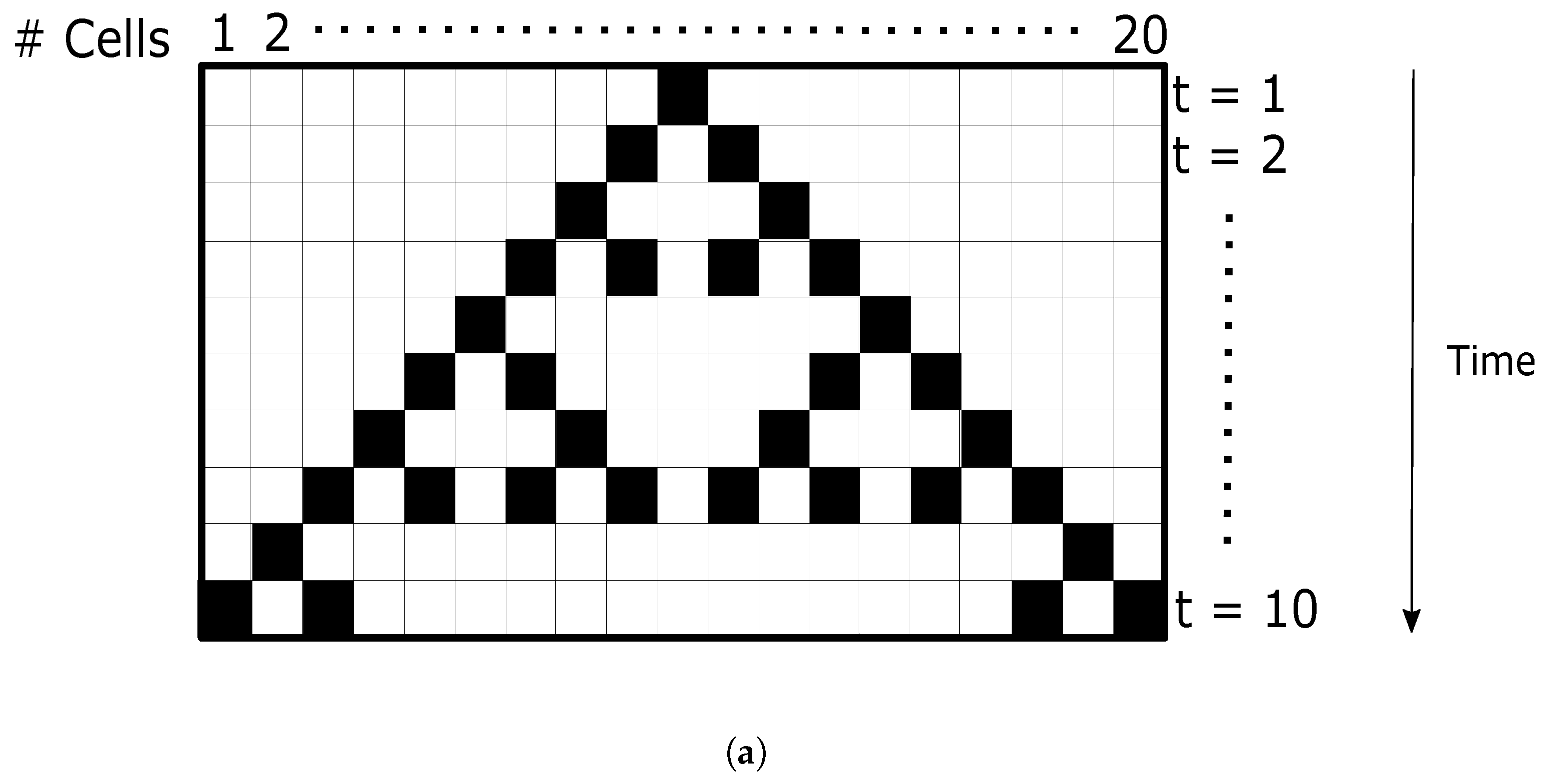
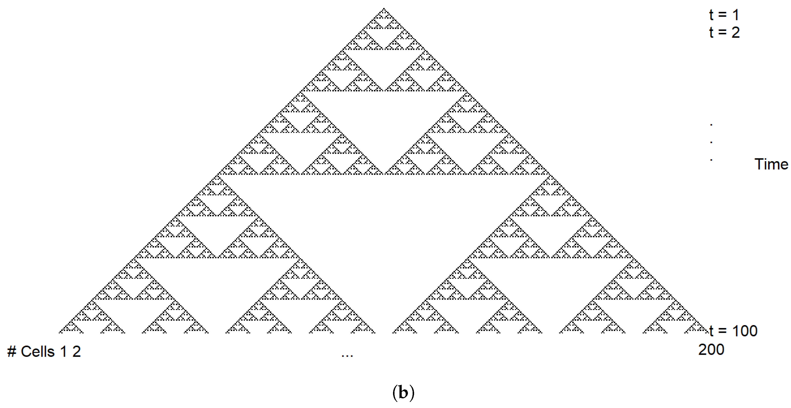
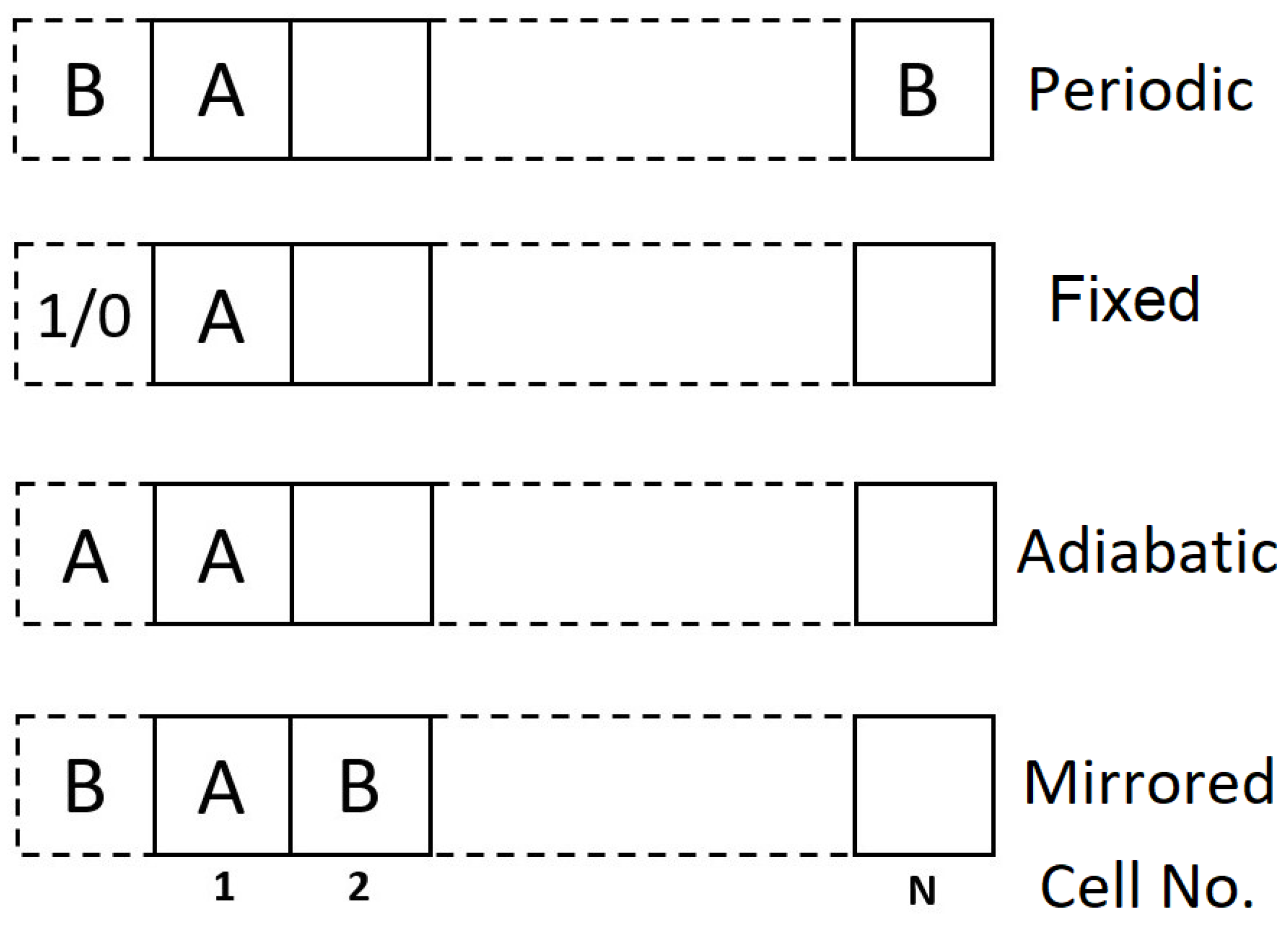

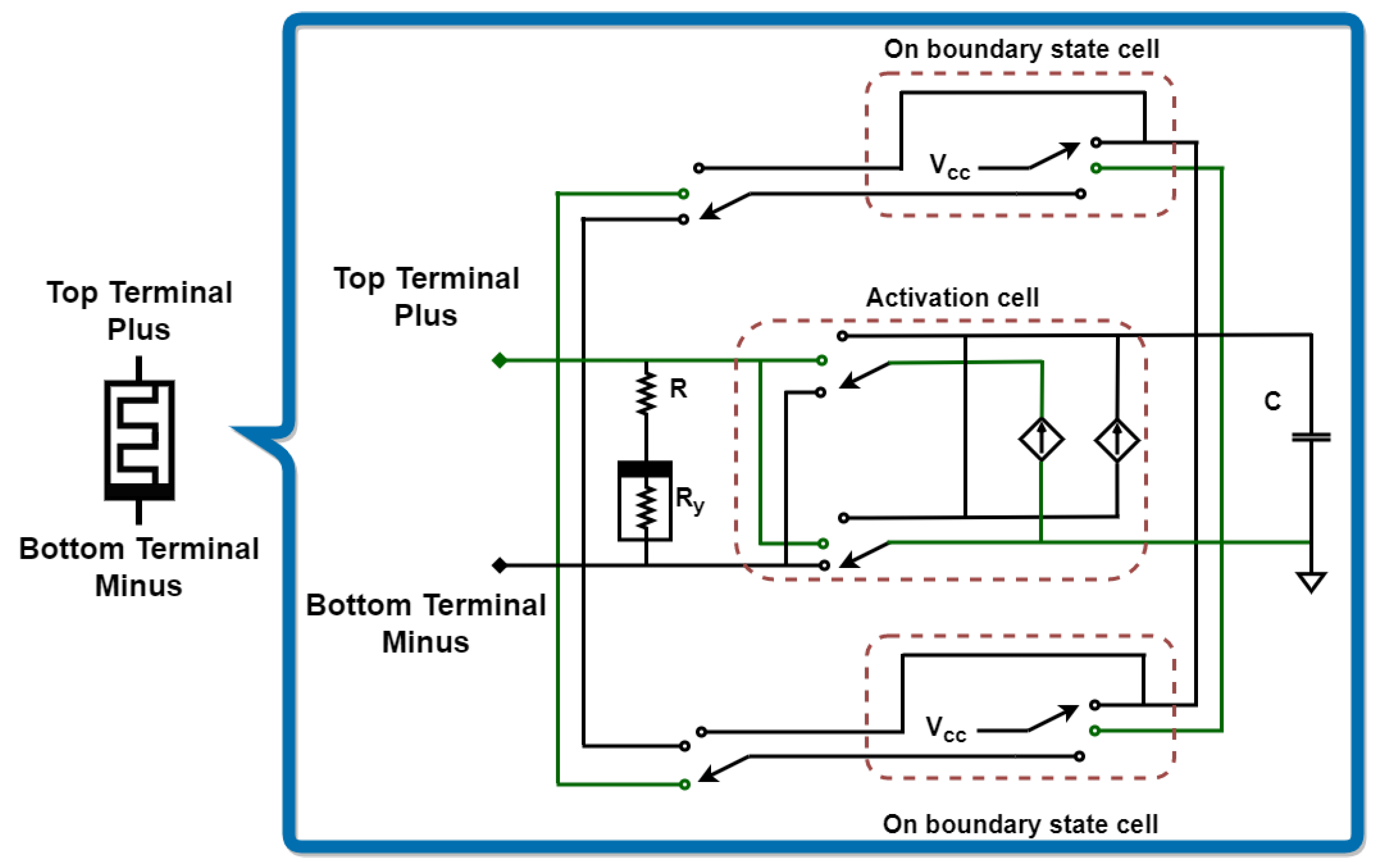

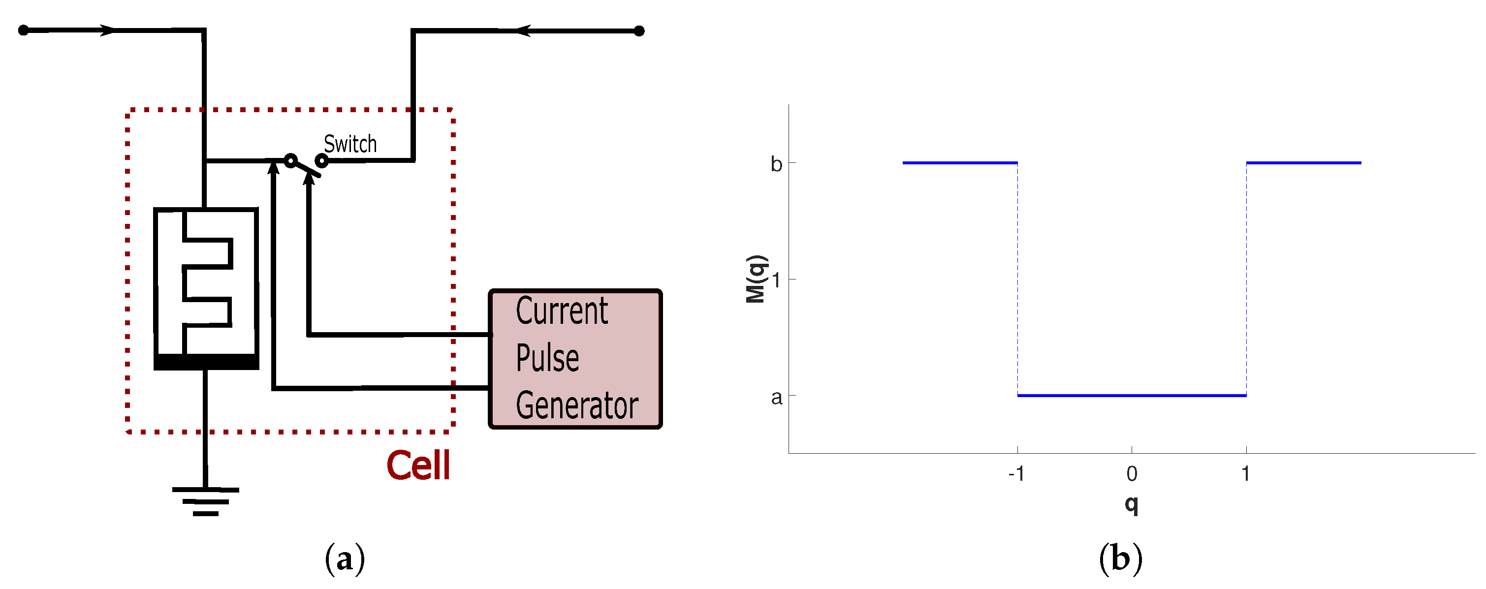
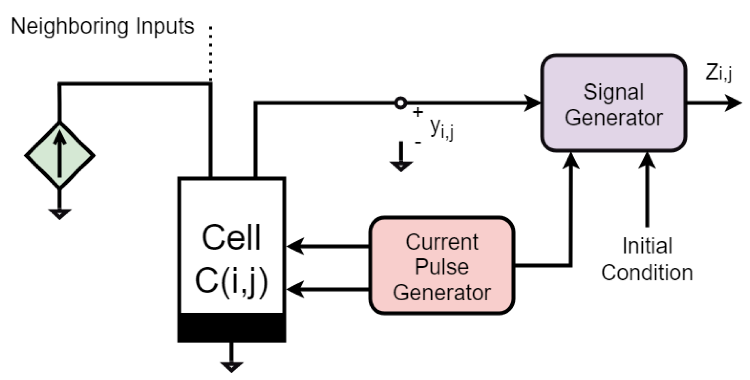
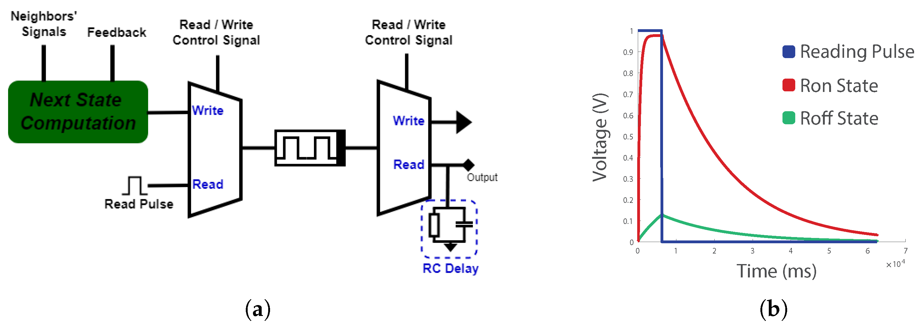
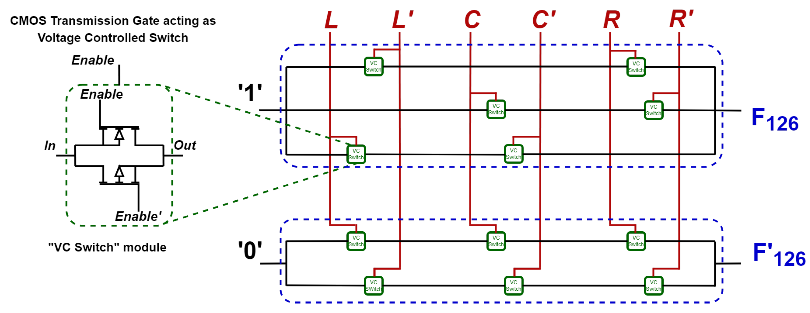

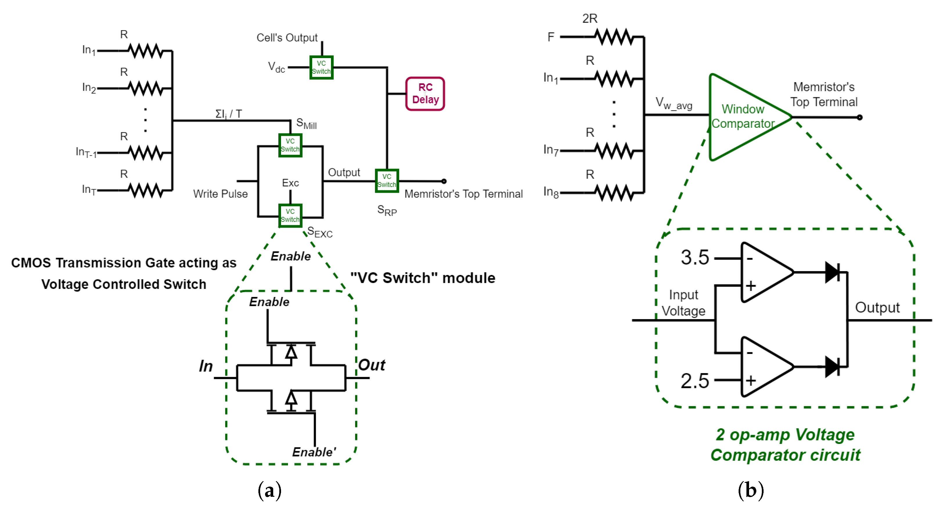
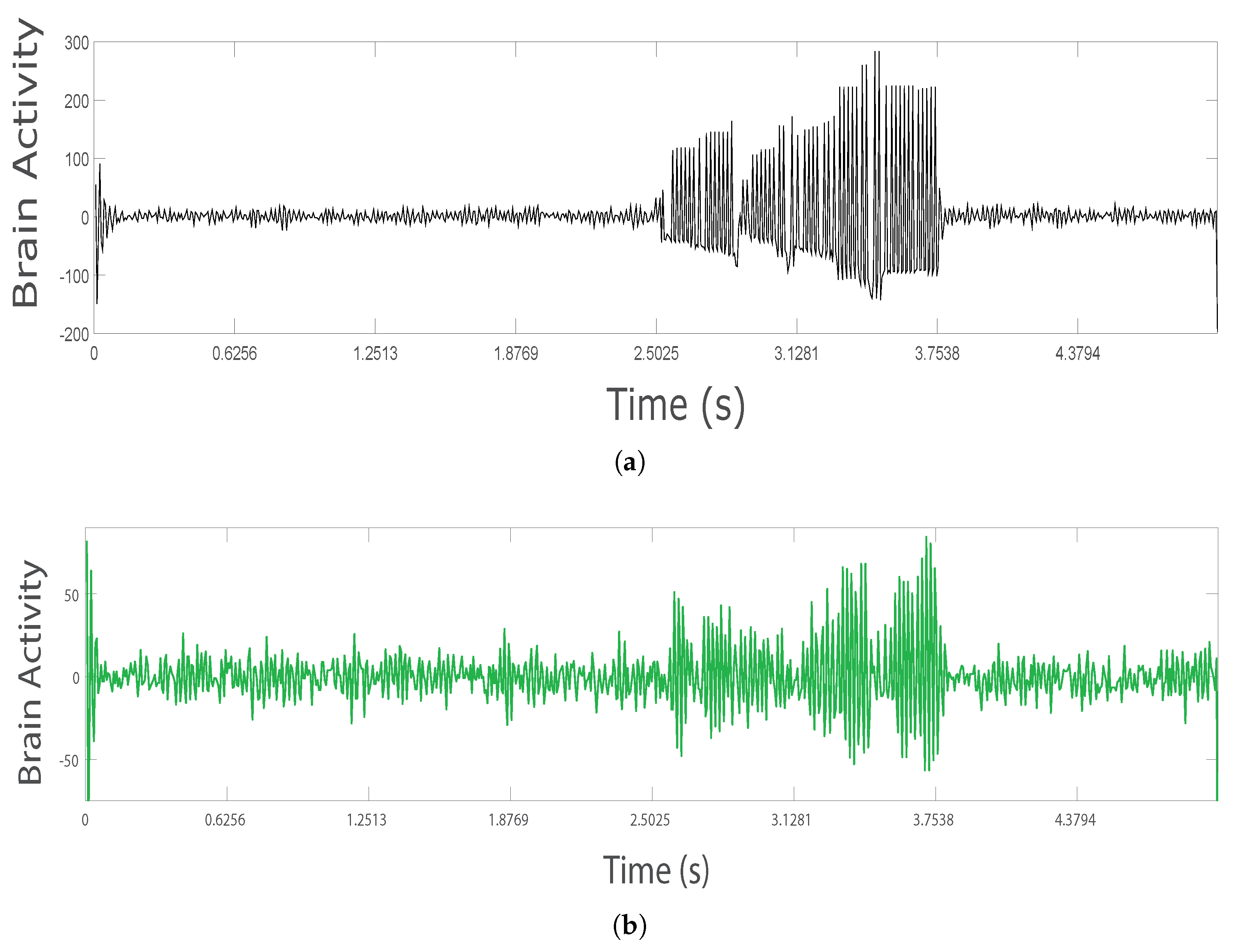
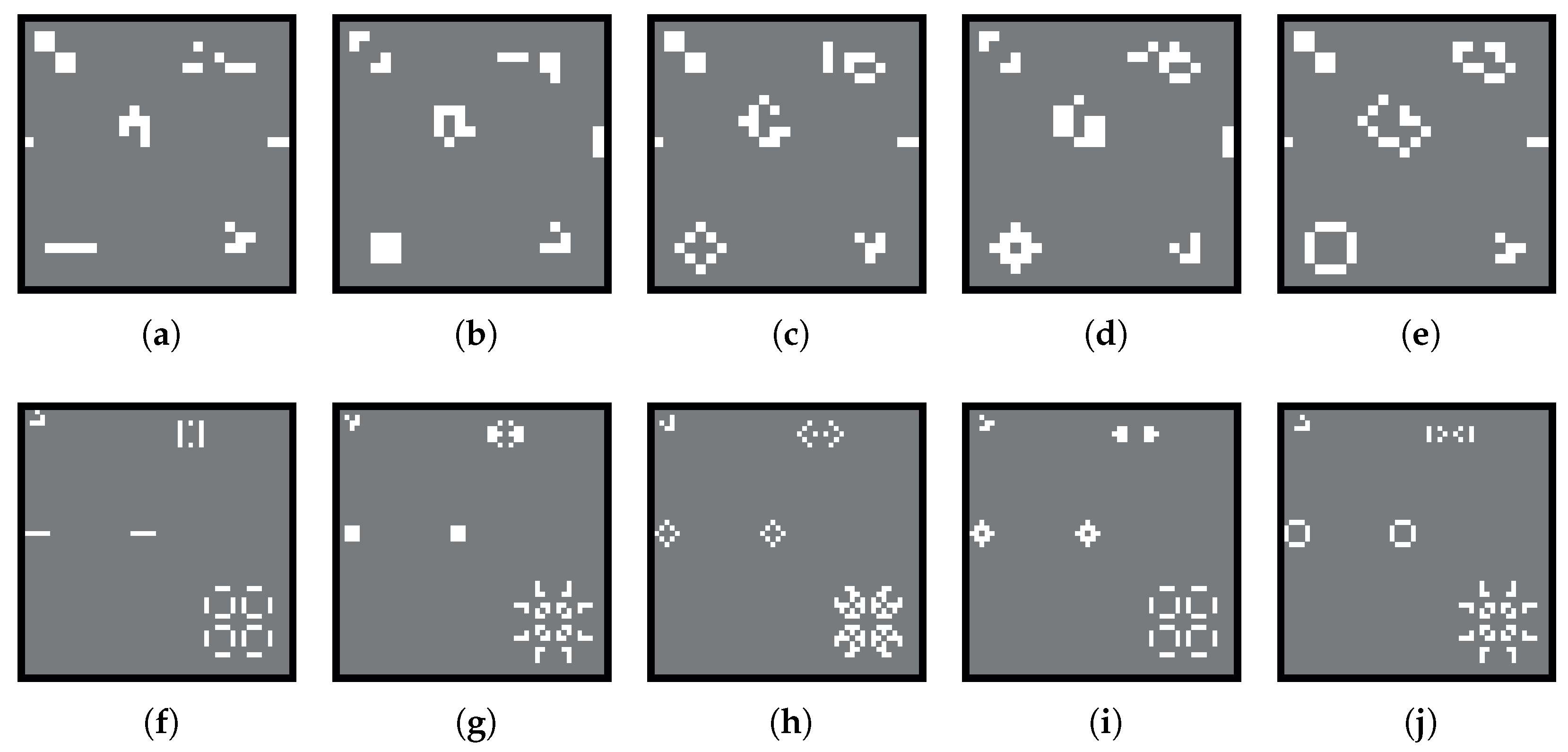
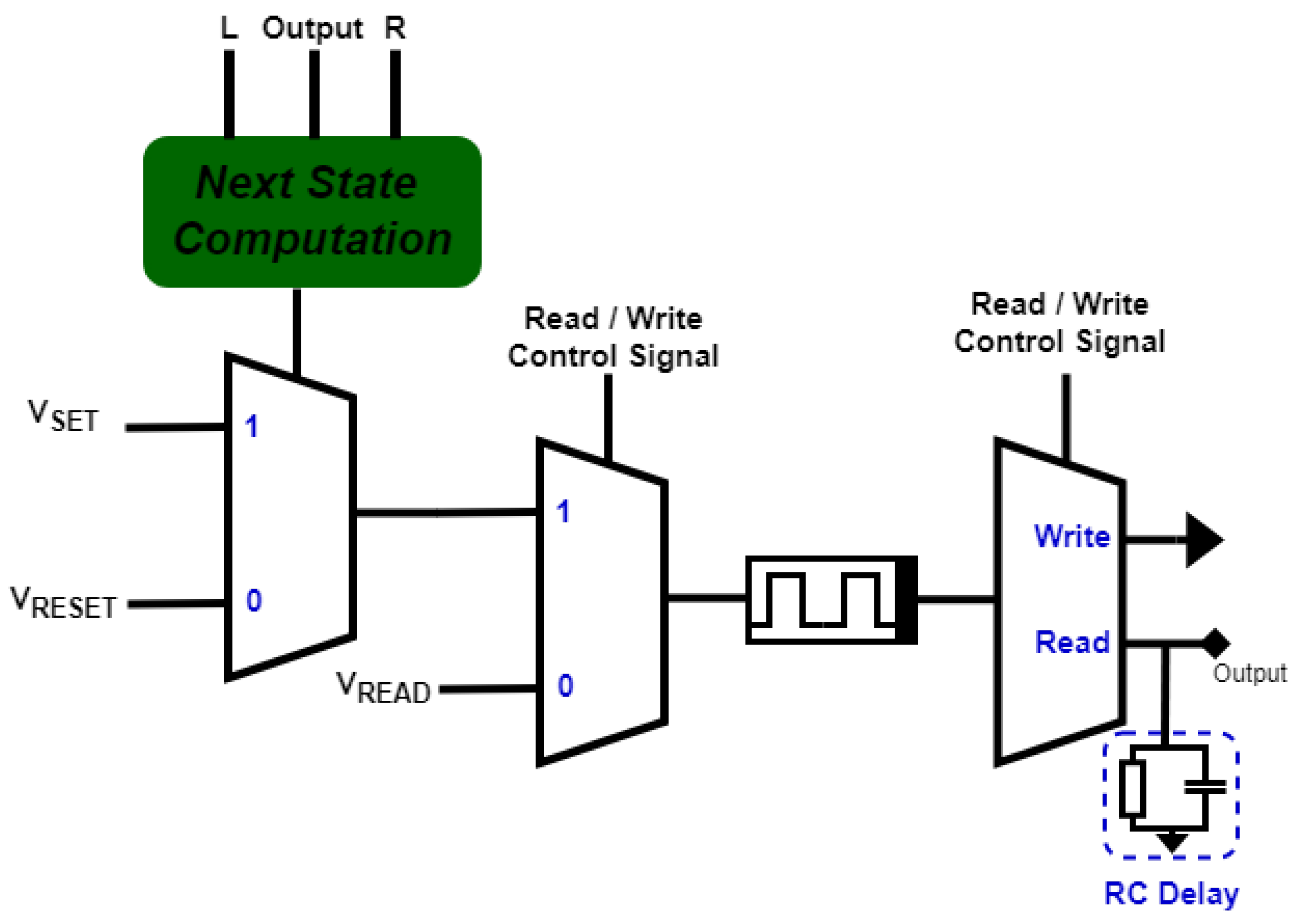

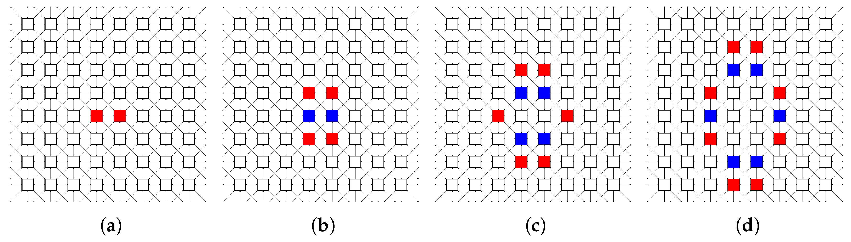
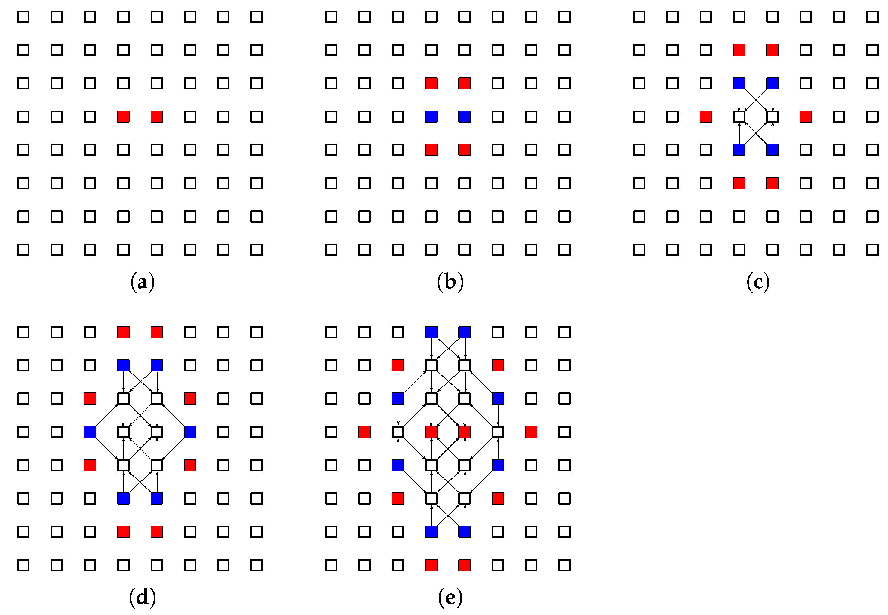
Disclaimer/Publisher’s Note: The statements, opinions and data contained in all publications are solely those of the individual author(s) and contributor(s) and not of MDPI and/or the editor(s). MDPI and/or the editor(s) disclaim responsibility for any injury to people or property resulting from any ideas, methods, instructions or products referred to in the content. |
© 2023 by the authors. Licensee MDPI, Basel, Switzerland. This article is an open access article distributed under the terms and conditions of the Creative Commons Attribution (CC BY) license (https://creativecommons.org/licenses/by/4.0/).