
Wavelet and Earth Mover’s Distance Coupling Denoising Techniques


Abstract
:1. Introduction
2. Background Techniques
- ➢
- Starting from the wavelet coefficients of an image Y:
- ➢
- The wavelet threshold Tj at each wavelet level j is set to
- ➢
- The wavelet coefficients after soft thresholds are
- ➢
- The inverse discrete wavelet transform of thresholding wavelet coefficients is just the denoised image.
3. Proposed Methods
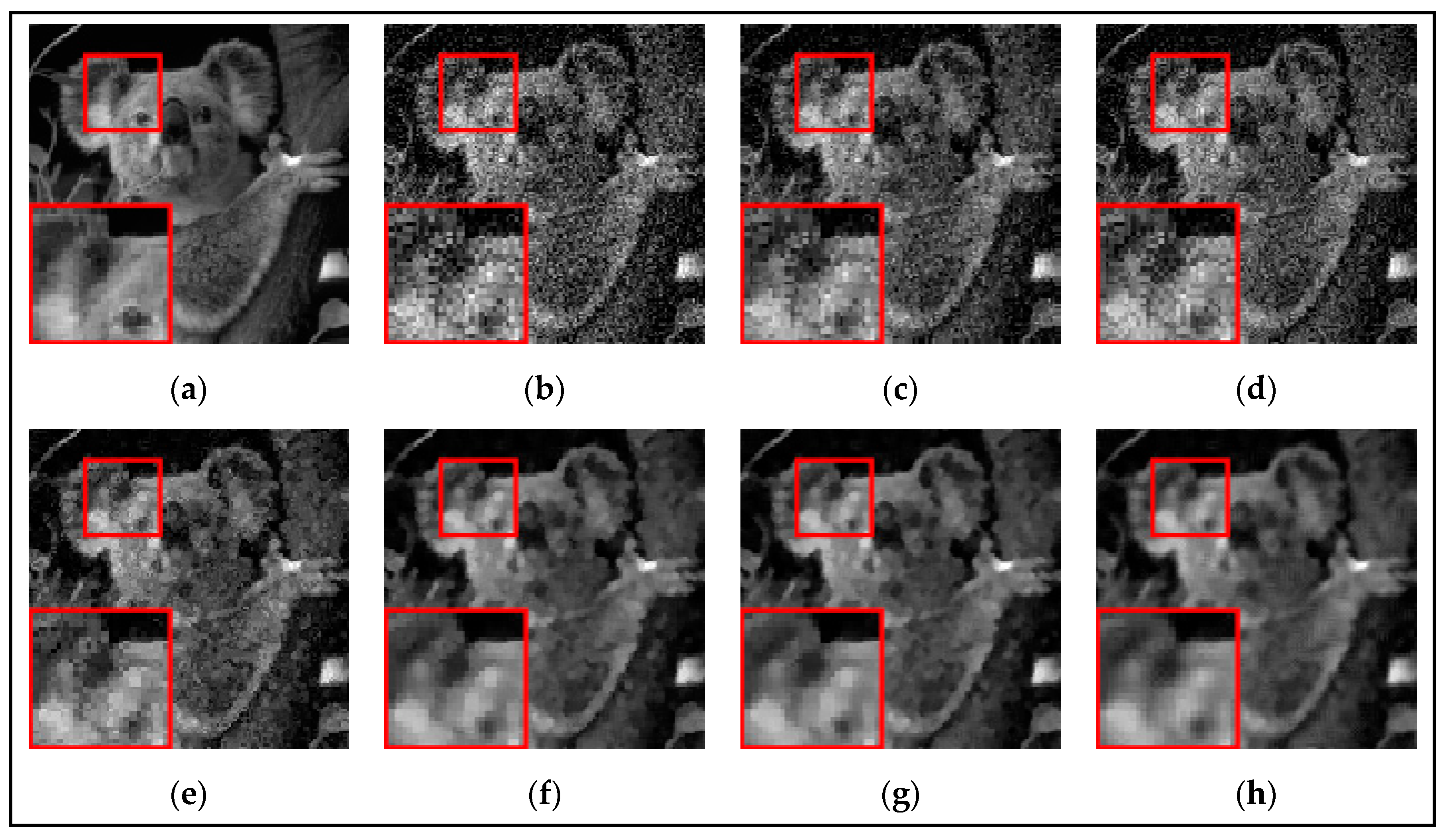
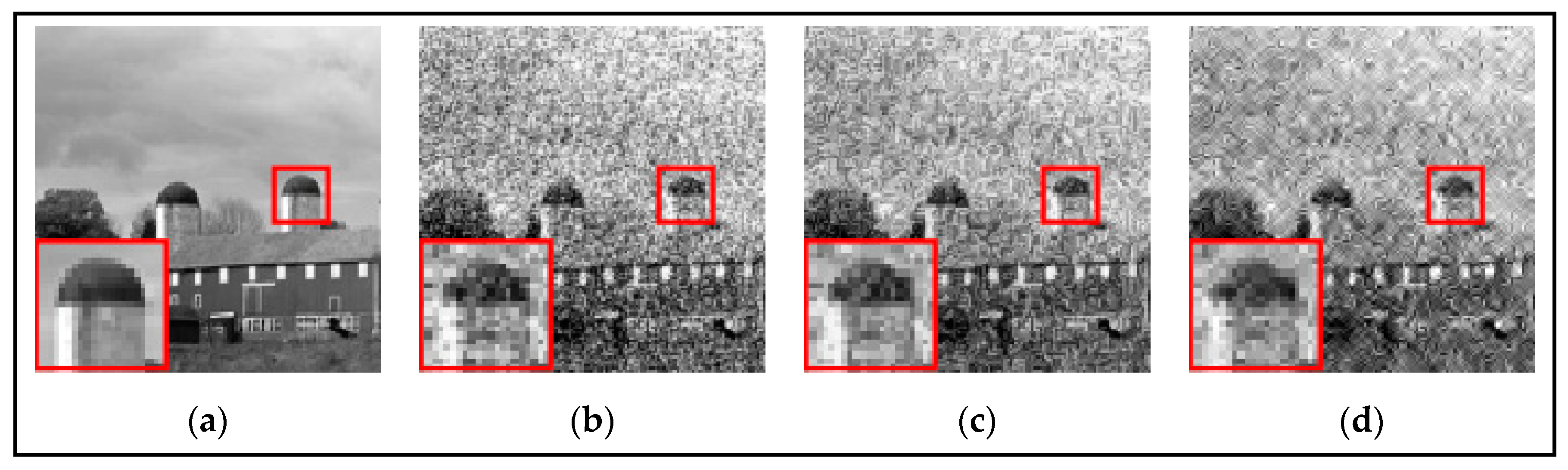
4. Denoising Experiments
4.1. Low Noise Level
4.2. Middle Noise Level
4.3. High Noise Level
4.4. Average Denoising Performance
4.5. Denoising Experiments on Kodak24 Dataset
4.6. Other Denoising Experiments
5. Conclusions
- ➢
- Our algorithm makes full use of not only the wavelet-denoising technique at a local scale, but also the interior similarity and redundancy embedded in the whole image, leading to our superior denoising performance over classic wavelet algorithms (DWT-H, DWT-S). Moreover, the use of joint bilateral filtering as a processing step, which detects high-frequency oscillations inside images, and then preserves image edges, further enhanced the denoising performance.
- ➢
- We used the earth mover’s distance as the similarity measure of small-scale patches of images. The earth mover’s distance (EMD) naturally extends the concept of distance between individual elements to the concept of distance between sets of elements. As the EMD tolerates the distortion of some moving features, it is well recognized as a much more robust clustering measure than the Euclidean distance, leading to our superior denoising performance over WNLM and NLMW, which use the Euclidean distance to measure the similarity.
Author Contributions
Funding
Institutional Review Board Statement
Informed Consent Statement
Data Availability Statement
Conflicts of Interest
References
- Meyer, Y.; Coifman, R.; Salinger, D. Wavelets: Calderón-Zygmund and Multilinear Operators; Cambridge University Press: Cambridge, UK, 1997. [Google Scholar]
- Mallat, S. A Wavelet Tour of Signal Processing: The Sparse Way; Academic Press: Cambridge, MA, USA, 2008. [Google Scholar]
- Daubechies, I. Ten Lectures on Wavelets; Society for Industrial and Applied Mathematics: Philadelphia, PA, USA, 1992. [Google Scholar]
- Gurkahraman, K.; Karakis, R.; Takci, H. A Novel Color Image Watermarking Method with Adaptive Scaling Factor Using Similarity-Based Edge Region. Tech. Sci. Press 2023, 47, 55–77. [Google Scholar] [CrossRef]
- Gowthami, V.; Bagan, K.B.; Pushpa, S.E.P. A novel approach towards high-performance image compression using multilevel wavelet transformation for heterogeneous datasets. J. Supercomput. 2023, 79, 2488–2518. [Google Scholar] [CrossRef]
- Syed, S.H.; Muralidharan, V. Feature extraction using Discrete Wavelet Transform for fault classification of planetary gearbox—A comparative study. Appl. Acoust. 2022, 188, 108572. [Google Scholar] [CrossRef]
- Samantaray, A.K.; Gorre, P.; Sahoo, P.K. Design of CSD based Bi-orthogonal Wavelet Filter Bank for Medical Image Retrieval. Adv. Electr. Eng. Electron. Energy 2023, 5, 100242. [Google Scholar] [CrossRef]
- Gonzalez, R.C.; Woods, R.E. Digital Image Processing, 3rd ed.; Prentice Hall Press: Englewod Cliffs, NJ, USA, 2007. [Google Scholar]
- Huang, T.; Yang, G.; Tang, G. A fast two-dimensional median filtering algorithm. IEEE Trans. Acoustic. Speech. Signal Process. 1979, 27, 13–18. [Google Scholar] [CrossRef]
- Tomasi, C.; Manduchi, R. Stereo matching as a nearest-neighbor problem. IEEE Trans. Pattern Anal. Mach. Intell. 1998, 20, 333–340. [Google Scholar] [CrossRef]
- Lee, J.S. Digital image enhancement and noise filtering by use of local statics. IEEE Trans. Pattern Anal. Mach. Intell. 2009, 2, 165–168. [Google Scholar]
- Perona, P.; Malik, J. Scale-space and edge detection using anisotropic diffusion. IEEE Trans. Pattern Anal. Mach. Intell. 2002, 12, 629–639. [Google Scholar] [CrossRef]
- Elad, M. On the origin of the bilateral filter and ways to improve it. Image Process. IEEE Trans. 2002, 11, 1141–1151. [Google Scholar] [CrossRef]
- Rabbani, H. Image denoising in steerable pyramid domain based on a local Laplace prior. Pattern Recognit. 2009, 42, 2181–2193. [Google Scholar] [CrossRef]
- Srivastava, M.; Anderson, C.L.; Freed, J.H. A New Wavelet Denoising Method for Selecting Decomposition Levels and Noise Thresholds. IEEE Access 2016, 4, 3862–3877. [Google Scholar] [CrossRef]
- Johnstone, M.; Silverman, B.W. Wavelet Threshold Estimators for Data with Correlated Noise. J. R. Stat. Soc. 1997, 59, 319–351. [Google Scholar] [CrossRef]
- Donoho, D.L.; Johnstone, I.M. Adapting to unknown smoothness via wavelet shrinkage. J. Am. Stat. Assoc. 1995, 90, 1200–1224. [Google Scholar] [CrossRef]
- Luiser, F.; Blu, T.; Unser, M. A new SURE approach to image denoising: Inters ale orthonormal wavelet thresholding. IEEE Trans Image Process. 2007, 9, 593–606. [Google Scholar] [CrossRef]
- Chang, S.G.; Yu, B.; Vetterli, M. Adaptive wavelet thresholding for image denoising and compression. IEEE Trans. Image Process 2000, 9, 1532–1546. [Google Scholar] [CrossRef]
- Blu, T.; Luisier, F. The SURE-LET approach to image denoising. IEEE Trans. Image Process 2007, 16, 2778–2786. [Google Scholar] [CrossRef]
- Chen, G.Y.; Bui, T.D.; Krzyzak, A. Image denoising with neighbor dependency and customized wavelet and threshold. Pattern Recognit. 2005, 38, 115–124. [Google Scholar] [CrossRef]
- Zhou, D.; Cheng, W. Image denoising with an optimal threshold and neighboring window. Pattern Recognit. 2008, 29, 1694–1697. [Google Scholar]
- Yi, T.H.; Li, H.N.; Zhao, X.Y. Noise Smoothing for Structural Vibration Test Signals Using an Improved Wavelet Thresholding Technique. Sensors 2012, 12, 11205–11220. [Google Scholar] [CrossRef]
- Liu, H.; You, Y.; Li, S.; He, D.; Sun, J.; Wang, J.; Hou, D. Denoising of Laser Self-Mixing Interference by Improved Wavelet Threshold for High Performance of Displacement Reconstruction. Photonics 2023, 10, 943. [Google Scholar] [CrossRef]
- Iqbal, M.Z.; Ghafoor, A.; Siddiqui, A.M. Satellite image resolution enhancement using dual-tree complex wavelet transform and nonlocal means. IEEE Geosci. Remote Sens. Lett. 2012, 10, 451–455. [Google Scholar] [CrossRef]
- Diwakar, M.; Kumar, M. CT image denoising using NLM and correlation-based wavelet packet thresholding. IET Image Process. 2018, 12, 708–715. [Google Scholar] [CrossRef]
- Diwakar, M.; Kumar, P.; Singh, A.K. CT image denoising using NLM and its method noise thresholding. Multimed. Tools Appl. 2020, 79, 14449–14464. [Google Scholar] [CrossRef]
- Suresh, K.V. An improved image denoising using wavelet transform. In Proceedings of the 2015 International Conference on Trends in Automation, Communications and Computing Technology, I-TACT-15, Bangalore, India, 21–22 December 2015. [Google Scholar]
- Singh, K.; Ranade, S.K.; Singh, C. Comparative performance analysis of various wavelet and nonlocal means-based approaches for image denoising. OPTIK-Int. J. Light Electron Opt. 2017, 131, 423–437. [Google Scholar] [CrossRef]
- Ye, S.; Mei, Y. Super resolution image reconstruction based on wavelet transform and non-local means. J. Comput. Appl. 2014, 34, 1182–1186. [Google Scholar]
- Rubner, Y.; Tomasi, C.; Guibas, L.J. The Earth Mover’s Distance as a Metric for Image Retrieval. Int. J. Comput. Vis. 2000, 40, 99–121. [Google Scholar] [CrossRef]
- Basha, B.; Nandi, D.; Kaur, K.N.; Arambam, P.; Gupta, S.; Segan, M.; Ranjan, P.; Kaul, U.; Janardhanan, R. Earth Mover’s Distance-Based Automated Disease Tagging of Indian ECGs. In Machine Learning in Information and Communication Technology: Proceedings of ICICT 2021, SMIT; Springer Nature Singapore: Singapore, 2023; Volume 498, pp. 3–19. [Google Scholar]
- Zhang, L.; Zhang, P. Research on aesthetic models based on neural architecture search. J. Intell. Fuzzy Syst. 2021, 8, 1–15. [Google Scholar] [CrossRef]
- Ling, Y.; Zhong, Z.; Cao, D.; Luo, Z.; Lin, Y.; Li, S.; Sebe, N. Cross-modality earth mover’s distance for visible thermal person re-identification. In Proceedings of the Computer Vision and Pattern Recognition, New Orleans, LA, USA, 18–24 June 2022; Volume 14. [Google Scholar]
- Yu, H.; Zhao, L.; Wang, H. Image Denoising Using Triradiate Shrinkage Filter in the Wavelet Domain and Joint Bilateral Filter in the Spatial Domain. IEEE Trans. Image Process. 2009, 18, 2364–2369. [Google Scholar]
- Karthikeyan, P.; Vasuki, S. Multiresolution joint bilateral filtering with modified adaptive shrinkage for image denoising. Multimed. Tools Appl. 2016, 75, 16135–16152. [Google Scholar]
- Zhang, M.; Gunturk, B.K. Multiresolution Bilateral Filtering for Image Denoising. IEEE Trans. Image Process. 2008, 17, 2324–2333. [Google Scholar] [CrossRef]
- Mahdaoui, A.E.; Ouahabi, A.; Moulay, M.S. Image Denoising Using a Compressive Sensing Approach Based on Regularization Constraints. Sensors 2022, 22, 2199. [Google Scholar] [CrossRef] [PubMed]


| σ = 10 | ||||||||||||
| Methods | DWT-H | DWT-S | WNLM | NLMW | Simple Version | Full Version | ||||||
| Image | PSNR | SSIM | PSNR | SSIM | PSNR | SSIM | PSNR | SSIM | PSNR | SSIM | PSNR | SSIM |
| 1 | 27.579 | 0.763 | 28.113 | 0.785 | 28.650 | 0.799 | 29.354 | 0.840 | 31.028 | 0.877 | 31.107 | 0.882 |
| 2 | 27.815 | 0.765 | 28.410 | 0.786 | 28.536 | 0.819 | 29.721 | 0.822 | 30.950 | 0.882 | 31.027 | 0.884 |
| 3 | 27.027 | 0.775 | 27.442 | 0.788 | 27.637 | 0.832 | 29.138 | 0.826 | 30.370 | 0.890 | 30.501 | 0.892 |
| 4 | 26.938 | 0.711 | 27.580 | 0.745 | 27.216 | 0.736 | 28.936 | 0.819 | 29.420 | 0.845 | 29.579 | 0.855 |
| 5 | 27.493 | 0.763 | 27.880 | 0.775 | 28.002 | 0.841 | 29.118 | 0.788 | 30.316 | 0.863 | 30.383 | 0.869 |
| 6 | 26.471 | 0.811 | 27.023 | 0.827 | 26.728 | 0.831 | 28.813 | 0.874 | 29.36 | 0.901 | 29.596 | 0.906 |
| 7 | 29.009 | 0.767 | 29.389 | 0.775 | 30.768 | 0.876 | 29.476 | 0.750 | 32.074 | 0.861 | 32.274 | 0.870 |
| 8 | 26.854 | 0.753 | 27.554 | 0.780 | 27.617 | 0.774 | 29.115 | 0.848 | 30.178 | 0.873 | 30.316 | 0.882 |
| 9 | 28.044 | 0.702 | 28.526 | 0.711 | 29.054 | 0.825 | 29.279 | 0.697 | 31.079 | 0.813 | 31.211 | 0.826 |
| 10 | 28.411 | 0.741 | 28.641 | 0.747 | 29.439 | 0.856 | 29.393 | 0.725 | 31.494 | 0.840 | 31.641 | 0.850 |
| 11 | 26.519 | 0.856 | 26.914 | 0.865 | 26.706 | 0.874 | 28.913 | 0.904 | 29.455 | 0.927 | 29.613 | 0.930 |
| 12 | 29.819 | 0.650 | 30.126 | 0.663 | 31.884 | 0.809 | 29.541 | 0.623 | 32.132 | 0.766 | 32.452 | 0.783 |
| 13 | 29.217 | 0.712 | 29.555 | 0.724 | 31.531 | 0.836 | 29.588 | 0.720 | 32.614 | 0.844 | 32.938 | 0.852 |
| 14 | 27.765 | 0.668 | 28.325 | 0.698 | 28.718 | 0.755 | 29.418 | 0.757 | 31.235 | 0.846 | 31.350 | 0.851 |
| 15 | 29.164 | 0.642 | 29.518 | 0.661 | 30.973 | 0.738 | 29.449 | 0.689 | 31.907 | 0.789 | 32.135 | 0.793 |
| 16 | 27.209 | 0.765 | 27.790 | 0.786 | 27.855 | 0.803 | 29.079 | 0.832 | 30.309 | 0.879 | 30.397 | 0.882 |
| 17 | 27.656 | 0.823 | 28.015 | 0.828 | 28.033 | 0.899 | 29.056 | 0.817 | 30.356 | 0.892 | 30.438 | 0.899 |
| 18 | 27.072 | 0.777 | 27.540 | 0.783 | 27.725 | 0.827 | 29.115 | 0.817 | 30.196 | 0.879 | 30.316 | 0.881 |
| 19 | 28.211 | 0.704 | 28.743 | 0.722 | 29.318 | 0.810 | 29.302 | 0.724 | 31.104 | 0.832 | 31.220 | 0.838 |
| 20 | 24.968 | 0.836 | 25.524 | 0.852 | 23.787 | 0.798 | 26.009 | 0.881 | 26.187 | 0.884 | 26.503 | 0.894 |
| 21 | 27.948 | 0.693 | 28.571 | 0.707 | 29.020 | 0.821 | 29.382 | 0.693 | 31.246 | 0.812 | 31.373 | 0.827 |
| 22 | 27.904 | 0.732 | 28.204 | 0.741 | 28.420 | 0.815 | 29.164 | 0.745 | 30.670 | 0.832 | 30.743 | 0.839 |
| 23 | 28.539 | 0.663 | 28.975 | 0.680 | 29.723 | 0.774 | 29.413 | 0.698 | 31.649 | 0.810 | 31.848 | 0.818 |
| 24 | 27.994 | 0.733 | 28.556 | 0.754 | 29.091 | 0.811 | 29.325 | 0.780 | 31.137 | 0.859 | 31.210 | 0.862 |
| σ = 20 | ||||||||||||
| Methods | DWT-H | DWT-S | WNLM | NLMW | Simple Version | Full Version | ||||||
| Image | PSNR | SSIM | PSNR | SSIM | PSNR | SSIM | PSNR | SSIM | PSNR | SSIM | PSNR | SSIM |
| 1 | 23.935 | 0.604 | 24.465 | 0.634 | 25.913 | 0.690 | 26.712 | 0.740 | 28.035 | 0.791 | 28.121 | 0.796 |
| 2 | 24.117 | 0.585 | 24.734 | 0.611 | 26.040 | 0.682 | 27.068 | 0.732 | 27.642 | 0.791 | 27.876 | 0.797 |
| 3 | 23.251 | 0.600 | 23.888 | 0.625 | 25.080 | 0.686 | 26.364 | 0.746 | 26.47 | 0.798 | 26.868 | 0.807 |
| 4 | 23.563 | 0.553 | 24.177 | 0.594 | 25.102 | 0.632 | 26.138 | 0.696 | 26.225 | 0.720 | 26.525 | 0.730 |
| 5 | 23.604 | 0.580 | 24.129 | 0.595 | 25.45 | 0.671 | 26.432 | 0.709 | 26.764 | 0.790 | 27.057 | 0.795 |
| 6 | 22.930 | 0.665 | 23.746 | 0.697 | 24.614 | 0.736 | 25.746 | 0.786 | 26.058 | 0.816 | 26.326 | 0.824 |
| 7 | 24.433 | 0.538 | 24.701 | 0.542 | 26.714 | 0.656 | 27.270 | 0.680 | 29.346 | 0.830 | 29.481 | 0.826 |
| 8 | 23.475 | 0.602 | 24.206 | 0.642 | 25.378 | 0.678 | 26.325 | 0.741 | 27.127 | 0.769 | 27.273 | 0.778 |
| 9 | 23.948 | 0.467 | 24.351 | 0.475 | 26.001 | 0.576 | 26.836 | 0.616 | 27.775 | 0.750 | 28.006 | 0.751 |
| 10 | 24.022 | 0.509 | 24.379 | 0.513 | 26.140 | 0.626 | 27.092 | 0.657 | 27.972 | 0.796 | 28.354 | 0.797 |
| 11 | 23.083 | 0.739 | 23.802 | 0.760 | 24.634 | 0.795 | 25.933 | 0.840 | 25.950 | 0.859 | 26.298 | 0.866 |
| 12 | 24.821 | 0.375 | 24.915 | 0.377 | 27.243 | 0.510 | 27.594 | 0.534 | 29.993 | 0.726 | 30.101 | 0.720 |
| 13 | 24.492 | 0.473 | 24.771 | 0.483 | 27.041 | 0.603 | 27.501 | 0.635 | 30.158 | 0.801 | 30.224 | 0.797 |
| 14 | 23.965 | 0.478 | 24.495 | 0.509 | 25.907 | 0.580 | 26.974 | 0.656 | 27.695 | 0.720 | 27.96 | 0.727 |
| 15 | 24.513 | 0.402 | 24.779 | 0.425 | 26.955 | 0.526 | 27.439 | 0.574 | 29.866 | 0.704 | 29.915 | 0.704 |
| 16 | 23.511 | 0.592 | 24.115 | 0.621 | 25.359 | 0.678 | 26.367 | 0.737 | 27.101 | 0.784 | 27.307 | 0.790 |
| 17 | 23.674 | 0.659 | 24.170 | 0.668 | 25.383 | 0.740 | 26.453 | 0.764 | 27.057 | 0.863 | 27.32 | 0.862 |
| 18 | 23.334 | 0.595 | 23.976 | 0.613 | 25.192 | 0.679 | 26.294 | 0.733 | 26.417 | 0.782 | 26.836 | 0.793 |
| 19 | 24.035 | 0.475 | 24.459 | 0.492 | 26.154 | 0.593 | 26.907 | 0.634 | 28.224 | 0.766 | 28.39 | 0.766 |
| 20 | 21.845 | 0.730 | 22.887 | 0.767 | 22.552 | 0.744 | 22.509 | 0.731 | 24.349 | 0.821 | 23.091 | 0.763 |
| 21 | 23.863 | 0.446 | 24.403 | 0.463 | 26.070 | 0.566 | 26.921 | 0.613 | 27.809 | 0.735 | 28.067 | 0.740 |
| 22 | 23.778 | 0.528 | 24.214 | 0.538 | 25.591 | 0.623 | 26.692 | 0.660 | 27.027 | 0.760 | 27.436 | 0.765 |
| 23 | 24.235 | 0.429 | 24.574 | 0.447 | 26.366 | 0.548 | 27.163 | 0.599 | 28.576 | 0.729 | 28.787 | 0.731 |
| 24 | 24.101 | 0.541 | 24.550 | 0.563 | 26.096 | 0.641 | 26.864 | 0.687 | 28.065 | 0.772 | 28.192 | 0.774 |
| σ = 30 | ||||||||||||
| Methods | DWT-H | DWT-S | WNLM | NLMW | Simple Version | Full Version | ||||||
| Image | PSNR | SSIM | PSNR | SSIM | PSNR | SSIM | PSNR | SSIM | PSNR | SSIM | PSNR | SSIM |
| 1 | 20.284 | 0.441 | 21.745 | 0.476 | 24.064 | 0.587 | 25.413 | 0.675 | 26.225 | 0.718 | 26.258 | 0.719 |
| 2 | 20.474 | 0.415 | 21.882 | 0.454 | 24.166 | 0.585 | 25.660 | 0.674 | 26.054 | 0.718 | 26.069 | 0.724 |
| 3 | 19.737 | 0.453 | 20.912 | 0.463 | 22.703 | 0.565 | 24.679 | 0.680 | 24.698 | 0.711 | 24.641 | 0.714 |
| 4 | 20.279 | 0.416 | 21.462 | 0.431 | 23.284 | 0.515 | 24.750 | 0.614 | 24.767 | 0.636 | 24.784 | 0.636 |
| 5 | 19.937 | 0.428 | 21.221 | 0.454 | 23.312 | 0.576 | 24.921 | 0.654 | 25.165 | 0.705 | 25.183 | 0.713 |
| 6 | 19.725 | 0.523 | 20.868 | 0.542 | 22.499 | 0.621 | 24.150 | 0.718 | 24.470 | 0.744 | 24.412 | 0.743 |
| 7 | 20.231 | 0.348 | 21.895 | 0.401 | 24.859 | 0.575 | 26.126 | 0.641 | 27.314 | 0.740 | 27.425 | 0.756 |
| 8 | 20.089 | 0.455 | 21.438 | 0.477 | 23.414 | 0.555 | 24.952 | 0.664 | 25.493 | 0.691 | 25.478 | 0.686 |
| 9 | 19.934 | 0.303 | 21.505 | 0.329 | 23.989 | 0.475 | 25.481 | 0.560 | 25.991 | 0.638 | 26.052 | 0.654 |
| 10 | 20.051 | 0.342 | 21.435 | 0.373 | 23.850 | 0.537 | 25.684 | 0.615 | 25.935 | 0.695 | 25.963 | 0.711 |
| 11 | 19.884 | 0.604 | 20.830 | 0.621 | 22.324 | 0.694 | 24.287 | 0.788 | 24.310 | 0.801 | 24.216 | 0.799 |
| 12 | 20.252 | 0.199 | 22.158 | 0.244 | 25.710 | 0.440 | 26.644 | 0.491 | 28.009 | 0.610 | 28.263 | 0.637 |
| 13 | 20.297 | 0.294 | 21.983 | 0.338 | 25.124 | 0.514 | 26.395 | 0.590 | 27.852 | 0.699 | 27.977 | 0.715 |
| 14 | 20.337 | 0.340 | 21.716 | 0.350 | 23.985 | 0.465 | 25.591 | 0.584 | 25.975 | 0.621 | 26.002 | 0.628 |
| 15 | 20.167 | 0.241 | 22.031 | 0.279 | 25.380 | 0.444 | 26.537 | 0.520 | 27.919 | 0.608 | 28.135 | 0.623 |
| 16 | 19.861 | 0.423 | 21.351 | 0.457 | 23.488 | 0.567 | 25.037 | 0.672 | 25.483 | 0.705 | 25.523 | 0.708 |
| 17 | 20.128 | 0.517 | 21.282 | 0.552 | 23.266 | 0.670 | 24.975 | 0.730 | 25.336 | 0.792 | 25.364 | 0.801 |
| 18 | 19.813 | 0.438 | 21.062 | 0.449 | 22.895 | 0.553 | 24.706 | 0.665 | 24.751 | 0.691 | 24.738 | 0.696 |
| 19 | 20.004 | 0.308 | 21.664 | 0.349 | 24.411 | 0.509 | 25.719 | 0.583 | 26.533 | 0.669 | 26.607 | 0.683 |
| 20 | 19.193 | 0.631 | 19.732 | 0.603 | 20.384 | 0.606 | 21.398 | 0.663 | 22.330 | 0.726 | 21.301 | 0.655 |
| 21 | 20.000 | 0.288 | 21.623 | 0.308 | 24.220 | 0.459 | 25.568 | 0.550 | 26.149 | 0.621 | 26.220 | 0.638 |
| 22 | 19.856 | 0.373 | 21.253 | 0.399 | 23.363 | 0.528 | 25.222 | 0.609 | 25.286 | 0.668 | 25.307 | 0.680 |
| 23 | 20.391 | 0.279 | 21.836 | 0.301 | 24.594 | 0.460 | 25.968 | 0.543 | 26.738 | 0.625 | 26.836 | 0.640 |
| 24 | 20.396 | 0.381 | 21.853 | 0.416 | 24.320 | 0.542 | 25.603 | 0.625 | 26.362 | 0.684 | 26.434 | 0.693 |
| σ = 40 | ||||||||||||
| Methods | DWT-H | DWT-S | WNLM | NLMW | Simple Version | Full Version | ||||||
| Image | PSNR | SSIM | PSNR | SSIM | PSNR | SSIM | PSNR | SSIM | PSNR | SSIM | PSNR | SSIM |
| 1 | 20.662 | 0.434 | 21.608 | 0.453 | 23.064 | 0.537 | 24.245 | 0.610 | 24.202 | 0.617 | 25.307 | 0.666 |
| 2 | 20.408 | 0.425 | 21.176 | 0.438 | 22.473 | 0.558 | 24.149 | 0.600 | 24.184 | 0.700 | 25.603 | 0.712 |
| 3 | 19.879 | 0.438 | 20.637 | 0.436 | 21.754 | 0.508 | 23.063 | 0.599 | 23.313 | 0.658 | 23.755 | 0.686 |
| 4 | 20.659 | 0.407 | 21.371 | 0.416 | 22.504 | 0.480 | 23.364 | 0.538 | 24.030 | 0.570 | 24.226 | 0.588 |
| 5 | 20.129 | 0.420 | 20.987 | 0.434 | 22.299 | 0.516 | 23.357 | 0.582 | 23.910 | 0.688 | 24.650 | 0.736 |
| 6 | 19.964 | 0.517 | 20.719 | 0.522 | 21.734 | 0.582 | 22.575 | 0.636 | 22.667 | 0.645 | 23.372 | 0.693 |
| 7 | 20.740 | 0.362 | 22.042 | 0.406 | 23.966 | 0.531 | 24.483 | 0.564 | 26.369 | 0.758 | 27.070 | 0.786 |
| 8 | 20.257 | 0.436 | 21.215 | 0.450 | 22.472 | 0.509 | 23.473 | 0.584 | 23.691 | 0.590 | 24.545 | 0.635 |
| 9 | 20.225 | 0.301 | 21.494 | 0.320 | 23.106 | 0.423 | 24.040 | 0.485 | 25.426 | 0.678 | 25.581 | 0.711 |
| 10 | 20.385 | 0.344 | 21.248 | 0.361 | 22.731 | 0.474 | 24.022 | 0.618 | 24.819 | 0.722 | 25.446 | 0.760 |
| 11 | 20.025 | 0.599 | 20.463 | 0.596 | 21.345 | 0.653 | 22.548 | 0.716 | 22.299 | 0.721 | 23.131 | 0.757 |
| 12 | 20.620 | 0.205 | 22.230 | 0.244 | 24.550 | 0.375 | 25.288 | 0.423 | 28.216 | 0.696 | 28.683 | 0.737 |
| 13 | 20.743 | 0.305 | 22.152 | 0.343 | 24.233 | 0.470 | 24.843 | 0.511 | 26.916 | 0.701 | 27.875 | 0.743 |
| 14 | 20.629 | 0.338 | 21.482 | 0.338 | 22.978 | 0.445 | 24.191 | 0.508 | 25.344 | 0.640 | 25.798 | 0.640 |
| 15 | 20.344 | 0.238 | 22.015 | 0.273 | 24.201 | 0.384 | 25.162 | 0.449 | 27.778 | 0.629 | 28.391 | 0.661 |
| 16 | 20.220 | 0.419 | 21.315 | 0.441 | 22.726 | 0.523 | 23.595 | 0.592 | 24.410 | 0.640 | 24.732 | 0.659 |
| 17 | 20.595 | 0.534 | 21.213 | 0.554 | 22.411 | 0.651 | 23.285 | 0.663 | 23.797 | 0.797 | 24.655 | 0.819 |
| 18 | 20.063 | 0.430 | 20.924 | 0.427 | 22.122 | 0.502 | 23.164 | 0.586 | 23.691 | 0.652 | 24.049 | 0.674 |
| 19 | 20.209 | 0.304 | 21.586 | 0.339 | 23.381 | 0.445 | 24.264 | 0.507 | 25.677 | 0.664 | 26.262 | 0.707 |
| 20 | 18.981 | 0.580 | 19.108 | 0.537 | 19.485 | 0.540 | 20.274 | 0.578 | 20.941 | 0.655 | 20.593 | 0.612 |
| 21 | 20.247 | 0.275 | 21.619 | 0.291 | 23.360 | 0.389 | 24.225 | 0.477 | 25.712 | 0.654 | 25.971 | 0.699 |
| 22 | 19.923 | 0.362 | 20.933 | 0.377 | 22.262 | 0.464 | 23.675 | 0.540 | 24.163 | 0.672 | 24.805 | 0.714 |
| 23 | 21.336 | 0.303 | 22.247 | 0.315 | 24.122 | 0.446 | 24.595 | 0.472 | 26.433 | 0.670 | 26.664 | 0.688 |
| 24 | 21.098 | 0.395 | 21.999 | 0.415 | 23.607 | 0.521 | 24.049 | 0.544 | 25.095 | 0.659 | 25.812 | 0.683 |
| σ = 50 | ||||||||||||
| Methods | DWT-H | DWT-S | WNLM | NLMW | Simple Version | Full Version | ||||||
| Image | PSNR | SSIM | PSNR | SSIM | PSNR | SSIM | PSNR | SSIM | PSNR | SSIM | PSNR | SSIM |
| 1 | 20.199 | 0.421 | 21.312 | 0.437 | 22.328 | 0.505 | 23.173 | 0.545 | 23.964 | 0.603 | 24.395 | 0.621 |
| 2 | 19.799 | 0.412 | 20.659 | 0.425 | 21.540 | 0.524 | 23.142 | 0.607 | 23.437 | 0.663 | 24.742 | 0.668 |
| 3 | 19.48 | 0.427 | 20.310 | 0.411 | 21.110 | 0.473 | 21.587 | 0.541 | 22.533 | 0.608 | 22.913 | 0.630 |
| 4 | 20.173 | 0.395 | 20.881 | 0.395 | 21.643 | 0.448 | 22.396 | 0.494 | 23.136 | 0.533 | 23.492 | 0.553 |
| 5 | 19.683 | 0.409 | 20.653 | 0.417 | 21.562 | 0.482 | 21.918 | 0.585 | 23.081 | 0.631 | 23.775 | 0.677 |
| 6 | 19.560 | 0.501 | 20.364 | 0.498 | 21.080 | 0.546 | 20.997 | 0.521 | 22.353 | 0.631 | 22.462 | 0.629 |
| 7 | 20.426 | 0.367 | 21.959 | 0.410 | 23.325 | 0.513 | 24.588 | 0.663 | 25.468 | 0.711 | 25.868 | 0.718 |
| 8 | 19.829 | 0.422 | 20.855 | 0.427 | 21.721 | 0.473 | 22.484 | 0.507 | 23.389 | 0.577 | 23.752 | 0.575 |
| 9 | 19.937 | 0.298 | 21.365 | 0.312 | 22.559 | 0.400 | 23.814 | 0.547 | 24.623 | 0.618 | 24.800 | 0.638 |
| 10 | 20.002 | 0.340 | 20.914 | 0.350 | 21.937 | 0.442 | 22.562 | 0.600 | 23.819 | 0.657 | 24.372 | 0.688 |
| 11 | 19.616 | 0.588 | 19.916 | 0.566 | 20.530 | 0.613 | 20.199 | 0.598 | 22.045 | 0.704 | 22.172 | 0.706 |
| 12 | 20.261 | 0.205 | 22.281 | 0.251 | 23.997 | 0.359 | 26.538 | 0.583 | 27.150 | 0.625 | 27.605 | 0.667 |
| 13 | 20.349 | 0.306 | 22.070 | 0.344 | 23.604 | 0.449 | 25.164 | 0.599 | 25.993 | 0.653 | 26.634 | 0.679 |
| 14 | 20.153 | 0.330 | 21.098 | 0.322 | 22.167 | 0.412 | 23.695 | 0.527 | 24.269 | 0.587 | 24.985 | 0.588 |
| 15 | 19.921 | 0.236 | 22.012 | 0.272 | 23.628 | 0.362 | 26.098 | 0.539 | 26.809 | 0.574 | 27.293 | 0.607 |
| 16 | 19.934 | 0.412 | 21.139 | 0.424 | 22.180 | 0.493 | 23.105 | 0.553 | 23.782 | 0.603 | 23.984 | 0.616 |
| 17 | 20.219 | 0.534 | 20.762 | 0.544 | 21.567 | 0.624 | 21.306 | 0.658 | 22.950 | 0.757 | 23.626 | 0.760 |
| 18 | 19.747 | 0.420 | 20.651 | 0.405 | 21.533 | 0.472 | 22.154 | 0.545 | 22.938 | 0.599 | 23.302 | 0.623 |
| 19 | 19.802 | 0.300 | 21.475 | 0.334 | 22.764 | 0.418 | 23.879 | 0.556 | 24.863 | 0.608 | 25.364 | 0.647 |
| 20 | 18.591 | 0.548 | 18.457 | 0.474 | 18.740 | 0.480 | 18.446 | 0.435 | 19.820 | 0.562 | 19.943 | 0.550 |
| 21 | 19.873 | 0.267 | 21.522 | 0.280 | 22.810 | 0.359 | 24.449 | 0.551 | 24.902 | 0.582 | 25.240 | 0.635 |
| 22 | 19.509 | 0.352 | 20.601 | 0.360 | 21.543 | 0.432 | 22.262 | 0.560 | 23.244 | 0.608 | 23.910 | 0.656 |
| 23 | 21.050 | 0.314 | 22.044 | 0.315 | 23.368 | 0.426 | 24.688 | 0.549 | 25.614 | 0.625 | 25.750 | 0.628 |
| 24 | 20.722 | 0.391 | 21.699 | 0.406 | 22.818 | 0.495 | 23.548 | 0.562 | 24.300 | 0.618 | 24.911 | 0.633 |
| σ = 70 | ||||||||||||
| Methods | DWT-H | DWT-S | WNLM | NLMW | Simple Version | Full Version | ||||||
| Image | PSNR | SSIM | PSNR | SSIM | PSNR | SSIM | PSNR | SSIM | PSNR | SSIM | PSNR | SSIM |
| 1 | 19.550 | 0.384 | 20.292 | 0.407 | 20.975 | 0.464 | 22.100 | 0.480 | 22.161 | 0.509 | 22.591 | 0.516 |
| 2 | 18.918 | 0.380 | 19.493 | 0.401 | 20.097 | 0.485 | 21.187 | 0.530 | 22.312 | 0.578 | 22.707 | 0.548 |
| 3 | 19.095 | 0.395 | 19.692 | 0.387 | 20.310 | 0.442 | 20.742 | 0.467 | 21.119 | 0.510 | 21.257 | 0.507 |
| 4 | 19.269 | 0.355 | 19.739 | 0.362 | 20.282 | 0.407 | 21.515 | 0.431 | 21.388 | 0.458 | 21.869 | 0.458 |
| 5 | 19.313 | 0.380 | 19.973 | 0.393 | 20.639 | 0.449 | 21.005 | 0.499 | 21.534 | 0.524 | 21.712 | 0.530 |
| 6 | 19.072 | 0.461 | 19.628 | 0.465 | 20.159 | 0.505 | 20.251 | 0.464 | 20.737 | 0.540 | 20.924 | 0.537 |
| 7 | 20.079 | 0.353 | 21.170 | 0.398 | 22.154 | 0.490 | 23.081 | 0.549 | 23.647 | 0.554 | 23.460 | 0.615 |
| 8 | 19.214 | 0.385 | 19.906 | 0.393 | 20.540 | 0.434 | 21.493 | 0.448 | 21.728 | 0.486 | 22.104 | 0.493 |
| 9 | 19.641 | 0.273 | 20.764 | 0.301 | 21.697 | 0.383 | 22.601 | 0.434 | 23.105 | 0.460 | 22.997 | 0.506 |
| 10 | 19.505 | 0.318 | 20.167 | 0.334 | 20.924 | 0.415 | 21.569 | 0.488 | 21.958 | 0.540 | 22.142 | 0.505 |
| 11 | 18.911 | 0.541 | 19.108 | 0.531 | 19.546 | 0.572 | 19.448 | 0.544 | 20.410 | 0.619 | 20.541 | 0.620 |
| 12 | 20.124 | 0.196 | 21.668 | 0.247 | 22.961 | 0.344 | 24.574 | 0.443 | 25.201 | 0.464 | 24.977 | 0.500 |
| 13 | 19.999 | 0.290 | 21.272 | 0.332 | 22.372 | 0.423 | 23.568 | 0.483 | 24.053 | 0.512 | 24.081 | 0.552 |
| 14 | 19.460 | 0.300 | 20.118 | 0.303 | 20.864 | 0.375 | 22.543 | 0.442 | 22.296 | 0.458 | 22.964 | 0.483 |
| 15 | 19.876 | 0.222 | 21.525 | 0.265 | 22.788 | 0.344 | 24.294 | 0.430 | 24.978 | 0.451 | 24.698 | 0.468 |
| 16 | 19.661 | 0.382 | 20.516 | 0.399 | 21.308 | 0.459 | 22.087 | 0.486 | 22.487 | 0.513 | 22.406 | 0.524 |
| 17 | 19.485 | 0.510 | 19.783 | 0.520 | 20.323 | 0.586 | 20.362 | 0.568 | 21.116 | 0.607 | 21.510 | 0.664 |
| 18 | 19.346 | 0.383 | 20.032 | 0.385 | 20.690 | 0.443 | 21.273 | 0.474 | 21.584 | 0.504 | 21.680 | 0.496 |
| 19 | 19.625 | 0.284 | 20.899 | 0.320 | 21.881 | 0.395 | 22.675 | 0.449 | 23.290 | 0.482 | 23.180 | 0.502 |
| 20 | 17.836 | 0.473 | 17.795 | 0.423 | 18.031 | 0.427 | 17.977 | 0.409 | 18.697 | 0.511 | 18.975 | 0.485 |
| 21 | 19.700 | 0.248 | 20.927 | 0.267 | 21.903 | 0.337 | 23.181 | 0.440 | 23.442 | 0.462 | 23.425 | 0.457 |
| 22 | 19.231 | 0.325 | 20.000 | 0.341 | 20.716 | 0.403 | 21.301 | 0.463 | 21.698 | 0.496 | 21.925 | 0.497 |
| 23 | 20.309 | 0.300 | 20.919 | 0.307 | 21.797 | 0.401 | 23.344 | 0.440 | 23.664 | 0.528 | 23.697 | 0.460 |
| 24 | 19.847 | 0.355 | 20.495 | 0.380 | 21.236 | 0.454 | 22.379 | 0.474 | 22.449 | 0.527 | 22.875 | 0.501 |
| Noise Levels | DWT-H | DWT-S | WNLM | NLMW | Simple Version | Full Version |
|---|---|---|---|---|---|---|
| σ = 10 | 27.735/0.742 | 28.205/0.757 | 28.601/0.815 | 29.129/0.777 | 30.687/0.854 | 30.841/0.861 |
| σ = 20 | 23.772/0.549 | 24.287/0.569 | 25.707/0.644 | 26.566/0.687 | 27.572/0.778 | 27.742/0.779 |
| σ = 30 | 20.055/0.393 | 21.447/0.419 | 23.734/0.543 | 25.228/0.629 | 25.799/0.688 | 25.800/0.694 |
| σ = 40 | 20.348/0.390 | 21.324/0.405 | 22.787/0.496 | 23.747/0.557 | 24.712/0.670 | 25.291/0.698 |
| σ = 50 | 19.951/0.383 | 21.042/0.390 | 22.086/0.466 | 23.008/0.559 | 23.938/0.623 | 24.387/0.641 |
| σ = 70 | 19.461/0.353 | 20.245/0.369 | 21.008/0.434 | 21.856/0.472 | 22.295/0.513 | 22.446/0.518 |
| Noise Levels | DWT-H | DWT-S | WNLM | NLMW | Simple Version | Full Version |
|---|---|---|---|---|---|---|
| σ = 10 | 27.51/0.754 | 27.98/0.772 | 28.40/0.811 | 29.14/0.803 | 30.50/0.863 | 30.54/0.886 |
| σ = 20 | 23.64/0.570 | 24.19/0.594 | 25.53/0.659 | 26.49/0.711 | 27.44/0.765 | 27.62/0.786 |
| σ = 30 | 19.97/0.411 | 21.36/0.438 | 23.59/0.552 | 25.12/0.645 | 25.56/0.677 | 25.68/0.698 |
| σ = 40 | 19.88/0.393 | 20.90/0.405 | 21.91/0.478 | 22.95/0.552 | 23.30/0.559 | 24.28/0.632 |
| σ = 50 | 22.02/0.515 | 20.90/0.405 | 21.91/0.478 | 22.95/0.552 | 23.30/0.560 | 24.05/0.654 |
| σ = 70 | 19.42/0.370 | 20.14/0.380 | 20.88/0.441 | 21.32/0.448 | 21.77/0.466 | 22.31/0.505 |
| Noise Levels | DWT-H | DWT-S | WNLM | NLMW | Simple Version | Full Version |
|---|---|---|---|---|---|---|
| λ = 0.4 | 23.94/0.527 | 24.43/0.548 | 26.00/0.631 | 26.87/0.678 | 28.17/0.757 | 28.43/0.779 |
| λ = 5 | 23.52/0.524 | 23.97/0.545 | 25.39/0.627 | 26.13/0.674 | 27.19/0.755 | 27.37/0.777 |
| λ = 10 | 22.52/0.519 | 22.88/0.540 | 23.95/0.621 | 24.46/0.667 | 25.13/0.748 | 25.24/0.770 |
Disclaimer/Publisher’s Note: The statements, opinions and data contained in all publications are solely those of the individual author(s) and contributor(s) and not of MDPI and/or the editor(s). MDPI and/or the editor(s) disclaim responsibility for any injury to people or property resulting from any ideas, methods, instructions or products referred to in the content. |
© 2023 by the authors. Licensee MDPI, Basel, Switzerland. This article is an open access article distributed under the terms and conditions of the Creative Commons Attribution (CC BY) license (https://creativecommons.org/licenses/by/4.0/).
Share and Cite
Zhang, Z.; Xu, X.; Crabbe, M.J.C. Wavelet and Earth Mover’s Distance Coupling Denoising Techniques. Electronics 2023, 12, 3588. https://doi.org/10.3390/electronics12173588
Zhang Z, Xu X, Crabbe MJC. Wavelet and Earth Mover’s Distance Coupling Denoising Techniques. Electronics. 2023; 12(17):3588. https://doi.org/10.3390/electronics12173588
Chicago/Turabian StyleZhang, Zhihua, Xudong Xu, and M. James C. Crabbe. 2023. "Wavelet and Earth Mover’s Distance Coupling Denoising Techniques" Electronics 12, no. 17: 3588. https://doi.org/10.3390/electronics12173588
APA StyleZhang, Z., Xu, X., & Crabbe, M. J. C. (2023). Wavelet and Earth Mover’s Distance Coupling Denoising Techniques. Electronics, 12(17), 3588. https://doi.org/10.3390/electronics12173588