
Sparse Non-Uniform Linear Array-Based Propagator Method for Direction of Arrival Estimation

Abstract
:1. Introduction
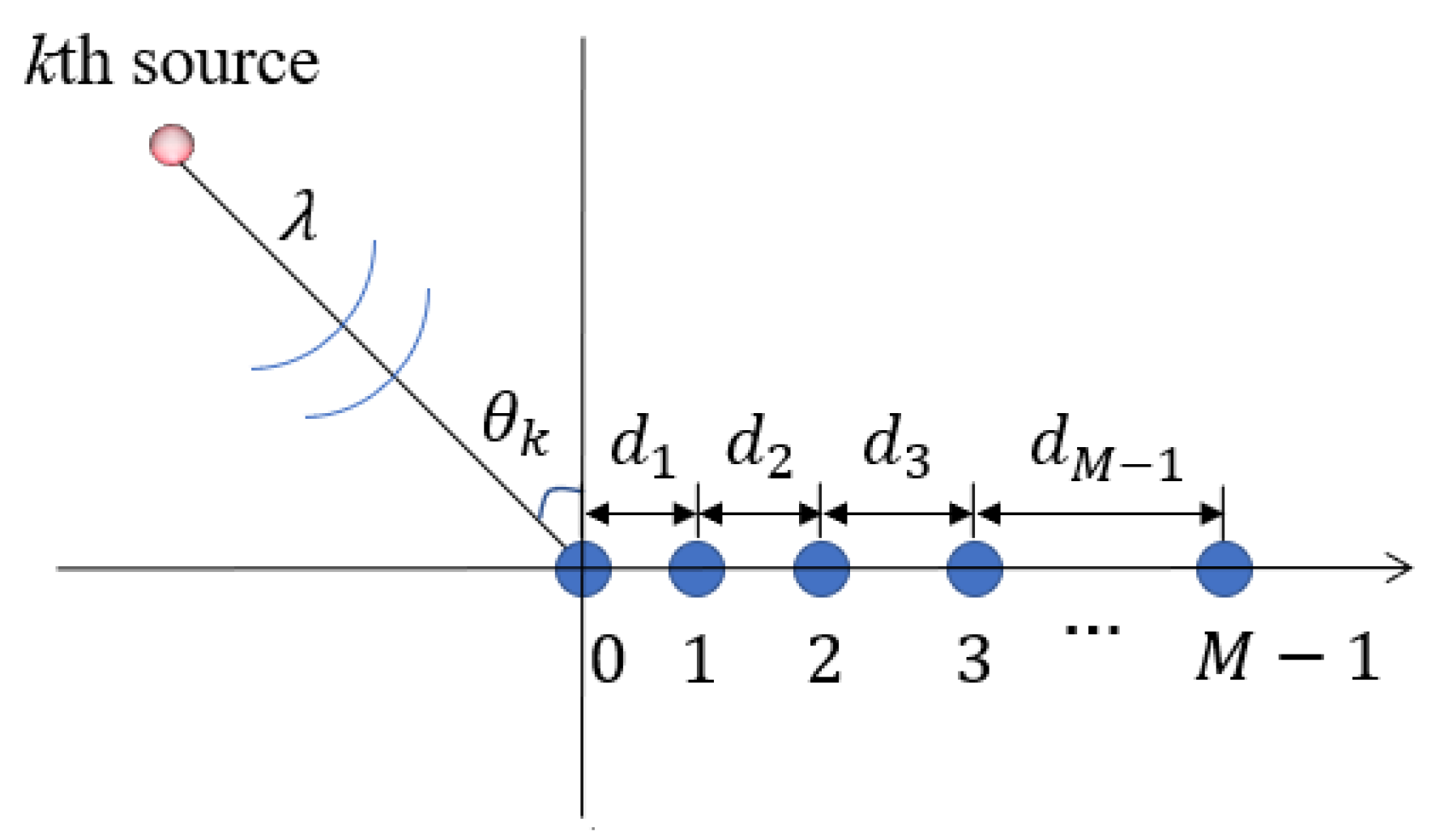
2. Signal Model
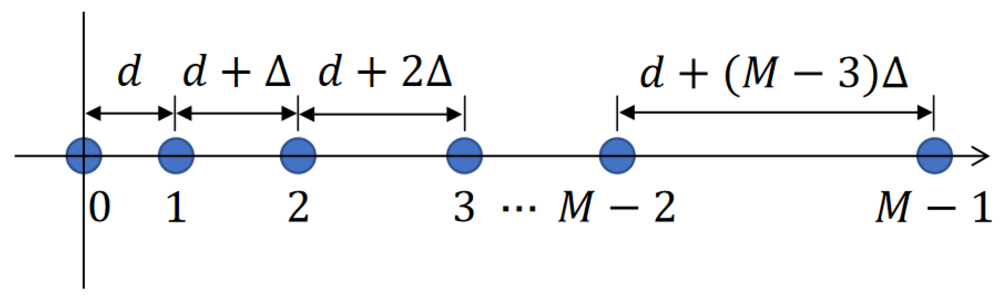
3. A Specific Configuration Scheme for Inter-Element Spacing
4. Proposed DOA Estimator
4.1. Fourth-Order Cumulant
4.2. Estimator with Source Number
4.3. Propagator Based on Elementary Transformation without Source Number
4.4. Estimator Based on Improved Propagator without Source Number
4.5. Refine Accuracy Based on the Projection onto an Irregular Toeplitz Set
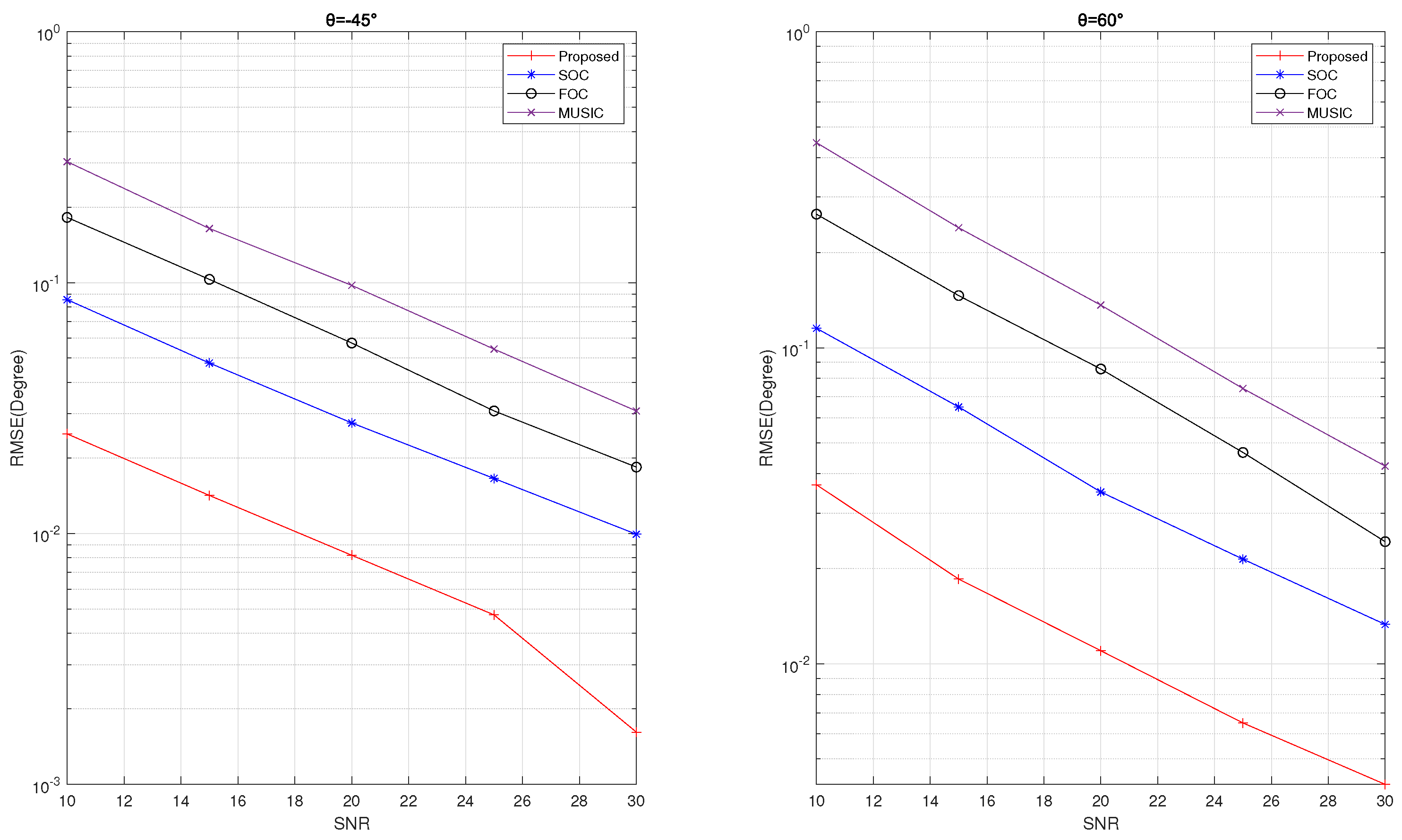
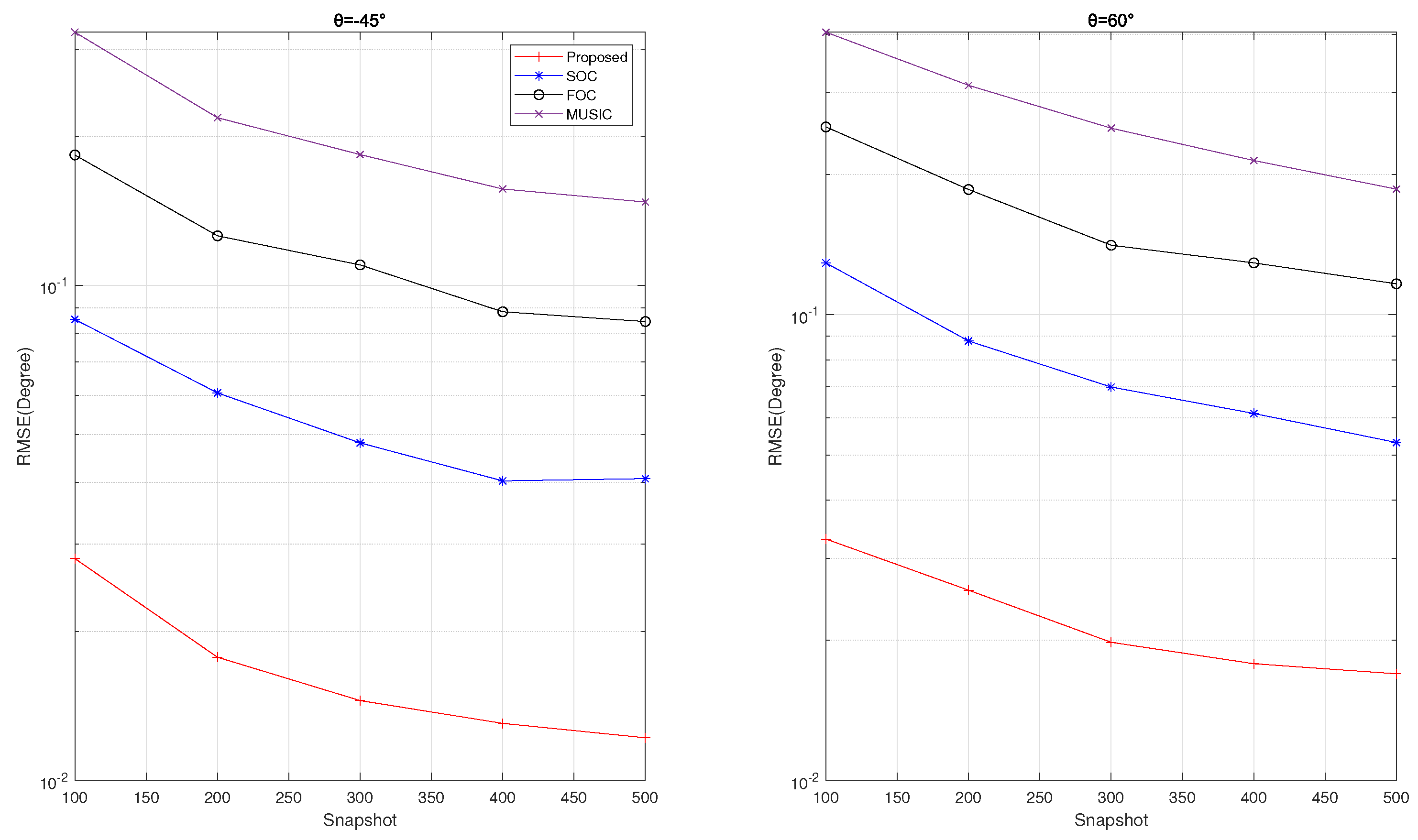
5. Experimental Results
6. Conclusions
Author Contributions
Funding
Institutional Review Board Statement
Informed Consent Statement
Data Availability Statement
Conflicts of Interest
References
- Blasone, G.P.; Colone, F.; Lombardo, P.; Wojaczek, P.; Cristallini, D. Dual cancelled channel STAP for target detection and DOA estimation in Passive Radar. Sensors 2021, 21, 4569. [Google Scholar] [CrossRef]
- Famoriji, O.J.; Shongwe, T. Subspace Pseudointensity Vectors Approach for DoA Estimation Using Spherical Antenna Array in the Presence of Unknown Mutual Coupling. Appl. Sci. 2022, 12, 10099. [Google Scholar] [CrossRef]
- Kuchar, A.; Tangemann, M.; Bonek, E. A real-time DOA-based smart antenna processor. IEEE Trans. Veh. Technol. 2002, 51, 1279–1293. [Google Scholar] [CrossRef]
- Suriyan, K.; Nagarajan, R.; Ghinea, G. Smart Antenna Optimization Techniques for Wireless Applications. Electronics 2023, 12, 2983. [Google Scholar] [CrossRef]
- Pirapaharan, K.; Prabhashana, W.H.S.C.; Medaranga, S.P.P.; Hoole, P.R.P.; Fernando, X. A New Generation of Fast and Low-Memory Smart Digital/Geometrical Beamforming MIMO Antenna. Electronics 2023, 12, 1733. [Google Scholar] [CrossRef]
- Ji, J.; Zhang, H.; Jiang, L.; Zhang, Y.; Yuan, Z.; Zhang, Z.; Chu, X.; Li, B. Seismic Behaviors of Novel Steel-Reinforced Concrete Composite Frames Prestressed with Bonding Tendons. Buildings 2023, 13, 2124. [Google Scholar] [CrossRef]
- Jing, Z.S.; Hudson, R.E.; Taciroglu, E.; Yao, K. Seismic-array signal processing for moving source localization. In Proceedings of the Conference on Advanced Signal Processing Algorithms, Architectures, and Implementations, San Diego, CA, USA, 26–30 August 2007. [Google Scholar]
- Savazzi, S.; Goratti, L.; Fontanella, D.; Nicoli, M.; Spagnolini, U. Pervasive UWB sensor networks for oil exploration. In Proceedings of the 2011 IEEE International Conference on Ultra-Wideband (ICUWB), IEEE, Bologna, Italy, 14–16 September 2011; pp. 225–229. [Google Scholar]
- Chalise, B.K.; Zhang, Y.D.; Himed, B. Compressed sensing based joint doa and polarization angle estimation for sparse arrays with dual-polarized antennas. In Proceedings of the 2018 IEEE Global Conference on Signal and Information Processing (GlobalSIP), Anaheim, CA, USA, 26–29 November 2018; pp. 251–255. [Google Scholar]
- Zhang, Y.; Zhang, L.Y.; Han, J.F.; Ban, Z.; Yang, Y. A new DOA estimation algorithm based on compressed sensing. Clust. Comput. 2019, 22, 895–903. [Google Scholar]
- Huang, H.; Yang, J.; Huang, H.; Song, Y.; Gui, G. Deep learning for super-resolution channel estimation and DOA estimation based massive MIMO system. IEEE Trans. Veh. Technol. 2018, 67, 8549–8560. [Google Scholar] [CrossRef]
- Gorcin, A.; Arslan, H. A two-antenna single RF front-end DOA estimation system for wireless communications signals. IEEE Trans. Antennas Propag. 2014, 62, 5321–5333. [Google Scholar] [CrossRef]
- Dakulagi, V. Single snapshot 2D-DOA estimation in wireless location system. Wirel. Pers. Commun. 2021, 117, 2327–2339. [Google Scholar] [CrossRef]
- Zhang, X.; Xu, L.; Xu, L.; Xu, D. Direction of departure (DOD) and direction of arrival (DOA) estimation in MIMO radar with reduced-dimension MUSIC. IEEE Commun. Lett. 2010, 14, 1161–1163. [Google Scholar] [CrossRef]
- Soldovieri, F.; Monte, L.L.; Erricolo, D. Tunnel detection and localisation via multi-monostatic radio frequency tomography using magnetic sources. IET Radar Sonar Navig. 2012, 6, 834–845. [Google Scholar] [CrossRef]
- Ma, Y.; Cao, X.; Wang, X. Enhanced DOA Estimation for MIMO radar in the Case of Limited Snapshots. In Proceedings of the 2020 IEEE 11th Sensor Array and Multichannel Signal Processing Workshop (SAM), IEEE, Hangzhou, China, 8–11 June 2020; pp. 1–5. [Google Scholar]
- Xu, F.; Morency, M.W.; Vorobyov, S.A. DOA estimation for transmit beamspace MIMO radar via tensor decomposition with Vandermonde factor matrix. IEEE Trans. Signal Process. 2022, 70, 2901–2917. [Google Scholar] [CrossRef]
- Ling, Y.; Gao, H.; Zhou, S.; Yang, L.; Ren, F. Robust Sparse Bayesian Learning-Based Off-Grid DOA Estimation Method for Vehicle Localization. Sensors 2020, 20, 302. [Google Scholar] [CrossRef]
- Cantarini, M.; Gabrielli, L.; Migliorelli, L.; Mancini, A.; Squartini, S. Beware the Sirens: Prototyping an Emergency Vehicle Detection System for Smart Cars. In Proceedings of the International Conference on Applied Intelligence and Informatics, Reggio Calabria, Italy, 1–3 September 2022; pp. 437–451. [Google Scholar]
- Schmidt, R. Multiple emitter location and signal parameter estimation. IEEE Trans. Antennas Propag. 1986, 34, 276–280. [Google Scholar] [CrossRef]
- Barabell, A. Improving the resolution performance of eigenstructure-based direction-finding algorithms. In Proceedings of the ICASSP ’83. IEEE International Conference on Acoustics, Speech, and Signal Processing, Boston, MA, USA, 14–16 April 1983; Volume 8, pp. 336–339. [Google Scholar]
- Richard, R.; Kailath, T. ESPRIT-estimation of signal parameters via rotational invariance techniques. IEEE Trans. Acoust. Speech Signal Process. 1989, 37, 984–995. [Google Scholar]
- Viberg, M.; Ottersten, B.; Kailath, T. Detection and estimation in sensor arrays using weighted subspace fitting. IEEE Trans. Signal Process. 1991, 39, 2436–2449. [Google Scholar] [CrossRef]
- Guo, S.; Cai, S.; Li, J.; Luo, D.; Xiong, X. High-order propagator-based DOA estimators using a coprime array without the source number. Signal Image Video Process. 2022, 17, 519–525. [Google Scholar] [CrossRef]
- Liang, J.; Liu, D. Passive localization of near-field sources using cumulant. IEEE Sens. J. 2009, 9, 953–960. [Google Scholar] [CrossRef]
- Liang, J.; Liu, D. Passive localization of mixed near-field and far-field sources using two-stage MUSIC algorithm. IEEE Trans. Signal Process. 2009, 58, 108–120. [Google Scholar] [CrossRef]
- Wang, B.; Zhao, Y.; Liu, J. Mixed-order MUSIC algorithm for localization of far-field and near-field sources. IEEE Signal Process. Lett. 2013, 20, 311–314. [Google Scholar] [CrossRef]
- Wang, K.; Wang, L.; Shang, J.R.; Qu, X.X. Mixed near-field and far-field source localization based on uniform linear array partition. IEEE Sens. J. 2016, 16, 8083–8090. [Google Scholar] [CrossRef]
- Li, J.; Wang, Y.; Ren, Z.; Gu, X.; Yin, M.; Wu, Z. DOA and range estimation using a uniform linear antenna array without a priori knowledge of the source number. IEEE Trans. Antennas Propag. 2020, 69, 2929–2939. [Google Scholar] [CrossRef]
- Wang, B.; Zheng, J. Cumulant-Based DOA Estimation of Noncircular Signals against Unknown Mutual Coupling. Sensors 2020, 20, 878. [Google Scholar] [CrossRef] [PubMed]
- Wu, H.T.; Yang, J.F.; Chen, F.K. Source number estimators using transformed Gerschgorin radii. IEEE Trans. Signal Process. 1995, 43, 1325–1333. [Google Scholar]
- Vertatschitsch, E.J.; Haykin, S. Impact of linear array geometry on direction-of-arrival estimation for a single source. IEEE Trans. Antennas Propag. 1991, 39, 576–584. [Google Scholar] [CrossRef]
- Huang, X.; Reilly, J.P.; Wong, M. Optimal design of linear array of sensors. In Proceedings of the ICASSP 91: 1991 International Conference on Acoustics, Speech, and Signal Processing, Toronto, ON, Canada, 14–17 April 1991; pp. 1405–1408. [Google Scholar]
- Moffet, A. Minimum-redundancy linear arrays. IEEE Trans. Antennas Propag. 1968, 16, 172–175. [Google Scholar] [CrossRef]
- Viberg, M.; Ottersten, B.; Nehorai, A. Performance analysis of direction finding with large arrays and finite data. IEEE Trans. Signal Process. 1995, 43, 469–477. [Google Scholar] [CrossRef]
- Mendel, J.M. Tutorial on higher-order statistics (spectra) in signal processing and system theory: Theoretical results and some applications. Proc. IEEE 1991, 79, 278–305. [Google Scholar] [CrossRef]
- Challa, R.N.; Shamsunder, S. High-order subspace-based algorithms for passive localization of near-field sources. In Proceedings of the Conference Record of The Twenty-Ninth Asilomar Conference on Signals, Systems and Computers, Pacific Grove, CA, USA, 30 October–1 November 1995. [Google Scholar]
- Li, J.; Dai, J.; Liang, Z.; Liu, D.; Guo, S.; Liu, Y. 2D DOA Estimation Through a Spiral Array Without the Source Number. Circuits Syst. Signal Process. 2022, 41, 3011–3022. [Google Scholar] [CrossRef]
- Ramírez, D.; Vazquez-Vilar, G.; López-Valcarce, R.; Vía, J.; Santamaría, I. Detection of rank-P signals in cognitive radio networks with uncalibrated multiple antennas. IEEE Trans. Signal Process. 2011, 59, 3764–3774. [Google Scholar] [CrossRef]
- Badawy, A.; Salman, T.; Elfouly, T.; Khattab, T.; Mohamed, A.; Guizani, M. Estimating the number of sources in white Gaussian noise: Simple eigenvalues based approaches. IET Signal Process. 2017, 11, 663–673. [Google Scholar] [CrossRef]
- Burnham, K.P.; Anderson, D.R. Multimodel inference: Understanding AIC and BIC in model selection. Sociol. Methods Res. 2004, 33, 261–304. [Google Scholar] [CrossRef]
- Zhao, L.; Krishnaiah, P.R.; Bai, Z. On detection of the number of signals in presence of white noise. J. Multivar. Anal. 1986, 20, 1–25. [Google Scholar] [CrossRef]
- Wagner, M.; Park, Y.; Gerstoft, P. Gridless DOA estimation and root-MUSIC for non-uniform linear arrays. IEEE Trans. Signal Process. 2021, 69, 2144–2157. [Google Scholar] [CrossRef]
- Pal, P.; Vaidyanathan, P.P. Nested arrays: A novel approach to array processing with enhanced degrees of freedom. IEEE Trans. Signal Process. 2010, 58, 4167–4181. [Google Scholar] [CrossRef]
- Pal, P.; Vaidyanathan, P.P. Multiple level nested array: An efficient geometry for 2q th order cumulant based array processing. IEEE Trans. Signal Process. 2011, 60, 1253–1269. [Google Scholar] [CrossRef]

| d | 0.1 | 0.2 | 0.3 | 0.4 | 0.5 | 0.6 | 0.7 | 0.8 | 0.9 | 1 | |
|---|---|---|---|---|---|---|---|---|---|---|---|
| 1 | 0.6781 | 0.3770 | 0.3668 | 0.3161 | 0.4226 | 0.2484 | 0.2718 | 0.2082 | 0.2678 | 0.1886 | |
| 2 | 0.2206 | 0.2423 | 0.2019 | 0.1841 | 0.1753 | 0.1835 | 0.1744 | 0.1531 | 0.1553 | 0.1536 | |
| 3 | 0.1557 | 0.1693 | 0.1642 | 0.1438 | 0.1399 | 0.1402 | 0.1511 | 0.1187 | 0.1235 | 0.1197 | |
| 4 | 0.1177 | 0.1413 | 0.1117 | 0.1632 | 0.1176 | 0.1232 | 0.1069 | 0.1427 | 0.1204 | 0.1067 | |
| 5 | 32.9941 | 0.1225 | 0.1110 | 0.1347 | 0.0940 | 0.1166 | 0.0869 | 0.1271 | 0.0753 | 0.1067 | |
| 6 | 0.1211 | 3.2585 | 0.0847 | 0.0727 | 0.0962 | 0.0899 | 0.0722 | 0.0680 | 0.0789 | 0.0872 | |
| 7 | 0.0670 | 0.0733 | 0.0733 | 0.0566 | 0.0660 | 0.0626 | 0.0657 | 0.0551 | 0.0536 | 0.0602 | |
| 8 | 0.0539 | 0.0501 | 0.0870 | 0.0481 | 0.0575 | 0.0447 | 0.0766 | 0.0507 | 0.0497 | 0.0360 | |
| 9 | 0.0575 | 0.0549 | 0.0542 | 0.0480 | 0.0667 | 0.0373 | 0.0647 | 0.0332 | 0.0762 | 0.0298 | |
| 10 | 63.3342 | 0.0547 | 0.0306 | 0.0703 | 0.0419 | 0.0467 | 0.0346 | 0.0471 | 0.0423 | 0.0281 | |
| M | 3 | 4 | 5 | 6 | 7 | 8 | 9 | 10 |
|---|---|---|---|---|---|---|---|---|
| 58.4 | 85.2 | 88.6 | 91 | 94.8 | 96.8 | 98 | 98.4 |
Disclaimer/Publisher’s Note: The statements, opinions and data contained in all publications are solely those of the individual author(s) and contributor(s) and not of MDPI and/or the editor(s). MDPI and/or the editor(s) disclaim responsibility for any injury to people or property resulting from any ideas, methods, instructions or products referred to in the content. |
© 2023 by the authors. Licensee MDPI, Basel, Switzerland. This article is an open access article distributed under the terms and conditions of the Creative Commons Attribution (CC BY) license (https://creativecommons.org/licenses/by/4.0/).
Share and Cite
Mo, H.; Tong, Y.; Wang, Y.; Wang, K.; Luo, D.; Li, W. Sparse Non-Uniform Linear Array-Based Propagator Method for Direction of Arrival Estimation. Electronics 2023, 12, 3755. https://doi.org/10.3390/electronics12183755
Mo H, Tong Y, Wang Y, Wang K, Luo D, Li W. Sparse Non-Uniform Linear Array-Based Propagator Method for Direction of Arrival Estimation. Electronics. 2023; 12(18):3755. https://doi.org/10.3390/electronics12183755
Chicago/Turabian StyleMo, Hanting, Yi Tong, Yanjiao Wang, Kaiwei Wang, Dongxiang Luo, and Wenlang Li. 2023. "Sparse Non-Uniform Linear Array-Based Propagator Method for Direction of Arrival Estimation" Electronics 12, no. 18: 3755. https://doi.org/10.3390/electronics12183755
APA StyleMo, H., Tong, Y., Wang, Y., Wang, K., Luo, D., & Li, W. (2023). Sparse Non-Uniform Linear Array-Based Propagator Method for Direction of Arrival Estimation. Electronics, 12(18), 3755. https://doi.org/10.3390/electronics12183755