Improved Smooth Watermarking Methods for Detecting Replay Attacks in Process Control Systems

Abstract

Network attack detection is a crucial issue in cyber–physical systems. One classical type of network attack is the replay attack. Although the watermarking scheme has proven to be effective in detecting replay attacks, it may confront numerous challenges when applied to process control systems. The watermarking signal, which consists of independent and identically distributed Gaussian noise sequences, responds slowly to industrial process control systems. To address this issue, two novel smooth watermarking methods are proposed. The smooth watermarking signals exhibit low-frequency characteristics, enabling them to effectively handle large inertia processes. The proposed schemes are validated through two simulated examples. These examples indicate that the proposed methods can significantly enhance detection efficiency while minimizing additional control performance loss.

1. Introduction

After decades of development, network technology has achieved very great progress. This makes it possible for it to be used in several control systems, such as cyber–physical systems (CPSs). The cyber and physical layers are connected through networks in these systems, which makes it easier to analyze and design control systems. In addition to the advantage, there has been growing concern about the security of these systems [1,2,3]. Control systems that are vulnerable to attacks can lead to severe consequences, such as serious economic losses [4,5].

Over the past few decades, there have been several attack incidents, for example, the attack on the Maroochy Shire Council’s sewage control system in Queensland in 2000 [6]. The StuxNet virus is another representative attack, which targets supervisory control and data acquisition systems used in several industrial and power systems [7]. Additionally, the Ukraine power outage in 2015 [8] and the security incident at the ‘Kemuri’ water company in 2016 [9] highlight the need for increased attention to CPS security. Hence, essential security schemes should be deployed in CPSs to fight against the attacks launched by some malicious users.

Among these attacks, one typical attack is called Denial-of-Service (DoS), which aims to disrupt network transmission [10]. Under a DoS attack, receivers cannot obtain any transmitted information, as the communication channels or infrastructures are paralyzed. Another representative attack is the replay attack, where the pre-recorded transmission is irregularly injected into networks by attackers [11]. This type of attack cannot be detected with traditional network defense technologies because the pre-recorded information is stolen from valid transmissions, such as involving the StuxNet virus [7]. In this context, secure strategies based on control theory should be developed to resist replay attacks.

Active detection schemes introduced from fault diagnoses are considered as the most effective solutions in detecting replay attacks. In these methods, probing signals will be injected into packets before transmission to facilitate the detection of attacks on the receiver side. A primary active detection method is the timestamp-based technology [12,13]. By embedding a timestamp in the head of the packets, replayed historical signals can be quickly identified by receivers. However, this method may not always be effective if attackers can tamper with the timestamps in stealing the packets [14].

In this context, another active detection scheme called watermark-based technology (physical watermark or dynamic watermark) was proposed to detect replay attacks [15]. This technology is inspired by digital watermarking techniques widely used in electronic documents to preserve private information. The watermarking signal is invisible to attackers because of its random characteristic, which greatly increases the difficulty of launching a replay attack. Therefore, it can be considered to be the most reliable detection technology to date. There are two types of watermarking signals according to their deployment positions. One is the sensor multiplicative watermark used to encrypt the sensor outputs [16]. The encrypted signals are then decrypted on the controller side. The most significant advantage of this watermarking is the zero-performance loss compared with its rival. However, theoretical studies on this watermarking are not yet complete.

Another type of watermarking scheme is known as a controller additive watermark. In this scheme, the watermarking signal is added to the control signal [15]. The watermarking signal can potentially degrade the efficiency of the control signal [17]. There have been sufficient theoretical works conducted in this area despite the negative impact on system performance [18]. The effectiveness of the watermarking method is addressed in [19], not only for single-input–single-output (SISO) systems but also for multi-input–multi-output (MIMO) systems with Gaussian noises. The watermarking strategy is also used to detect and distinguish replay attacks from other anomalies in nuclear power plants [20]. The effectiveness of the watermarking scheme is demonstrated in the context of power systems to secure the distributed measurements feeding automatic generation control (AGC) [21].

Other studies on generating watermarking signals have also been reported, such as periodic watermarking signals [22], online watermarking signals [23], time-varying watermarking signals [24], two-controller schemes [25], etc. Apart from the timestamp and watermarking-based technologies, other active detection schemes have also been investigated. For example, a hidden Markov model is utilized to replace watermarking signals by generating a set of random serial numbers [18].

Compared with the sensor multiplicative watermarking method, the controller additive watermarking scheme is considered easier to implement from an engineering perspective. It is worth noting that the watermarking method proposed in [18] can be applied to various CPSs, excluding process control systems [26,27]. These process systems may not be sensitive to the watermarking signal due to their large inertia characteristic. Therefore, applying a watermarking signal in these systems not only has ineffective attack detection but also results in reduced control performance. So, in summary, it is necessary to make some improvements if the watermarking signal is to be used in process control systems.

Motivated by the aforementioned reasons, two improved watermarking methods used for process control systems are proposed in this paper. The main contributions are outlined as follows:

(1) While numerous uses of the watermarking scheme exist in dynamic systems, there is a lack of research on process systems. In this paper, smoothing technologies are applied to increase the sensitivity of the process systems to watermarking signals. In this context, this problem may be solved with the proposed smooth watermarking and sliding smooth watermarking schemes, which can greatly extend the application of the watermarking method proposed in [18].

(2) The relationship between the performance loss and the watermarking signal is explicitly explored. The purpose is to minimize the performance loss while still achieving better attack detection efficiency by designing suitable smooth parameters.

The remainder of this paper is organized as follows: Section 2 introduces the system description. Section 3 presents the system model under attacks. Section 4 proposes two smooth watermarking methods for process control systems. Finally, Section 5 provides two examples to illustrate the effectiveness of the proposed smooth watermarking schemes.

Notations: $R$ and $Z$ denote the set of all real numbers and the set of integers, respectively. $R^n$ is the n-dimensional Euclidean space. $X^T$ represents the transpose of the matrix $X$. $X^{-1}$ represents the inverse of the matrix $X$. $I$ is the identity matrix with an appropriate dimension. $N\left(\mu ,{\sigma }^2\right)$ stands for Gaussian white noise with mean $\mu$ and variance ${\sigma }^2$.

2. System Description

In this section, the discrete system model considered in the paper is constructed. Additionally, the Kalman estimator and the LQG control scheme are introduced.

2.1. System Model and Kalman Estimator

Consider a discrete linear time-invariant (LTI) system,

$$x_{k+1}=A{x}_k+B{u}_k+{\omega }_k,$$

(1)

$$y_k=C{x}_k+{\nu }_k.$$

(2)

where $x_k\in R^n$ is the system state, $u_k\in R^n$ denotes the control input, and $y_k\in R^n$ means the system output. $A$, $B$, and $C$ are the system matrix, control matrix, and measurement matrix with appropriate dimensions. $\left\{{\omega }_k\sim N\left(0,Q\right)\right\}$ and $\left\{{\nu }_k~N\left(0,R\right)\right\}$ respectively represent process and measurement noise, and are independent of each other. $Q$ and $R$ are positive definite covariance matrices.

The Kalman estimator, an optimal filter based on the least mean square error, is used to effectively remove noise interference in (2). Being an online recursive algorithm, it does not need to store all the historical data but the data from the last moment. The Kalman estimator can be represented as

$${\hat{x}}_{k\mid k-1}=A{\hat{x}}_{k-1}+B{u}_{k-1},$$

(3)

$${\hat{x}}_k={\hat{x}}_{k\mid k-1}+K\left(y_k-C{\hat{x}}_{k\mid k-1}\right),$$

(4)

$$z_k\triangleq y_k-C{\hat{x}}_{k\mid k-1} ,$$

(5)

$$e_k\triangleq x_k-{\hat{x}}_k.$$

(6)

where ${\hat{x}}_{k\mid k-1}$ and ${\hat{x}}_k$ denote the prior estimation and optimal estimation of $x_k$, respectively. $z_k$ is the residual vector. And $e_k$ means the estimation error. The Kalman gain can be calculated as follows:

$$K=P{C}^T{\left(CP{C}^T+R\right)}^{-1},$$

(7)

where $P$ is the solution of the following Riccati equation:

$$P=AP{A}^T+Q-AP{C}^T{\left(CP{C}^T+R\right)}^{-1}CP{A}^T,$$

(8)

2.2. LQG Optimal Controller

In order to obtain the control signal, an LQG controller is used to minimize the following infinite horizon linear quadratic objective function:

$$J=\underset{N\to \infty }{\lim }E\left\{\frac{1}{N+1}\left[{\displaystyle \sum }_{k=0}^N\left(x_k^{T}W{x}_k+u_k^{T}U{u}_k\right)\right]\right\},$$

(9)

where $W$ and $U$ are positive semidefinite matrices. According to the separation theorem, an optimal control input $u_k^{*}$ is derived by solving the optimization problem mentioned above. The control input is the linear feedback of the optimal state estimation ${\hat{x}}_k$.

$$u_k^{*}=L{\hat{x}}_k,$$

(10)

where $L$ can be described as

$$L=-{\left(B^{T}SB+U\right)}^{-1}{B}^{T}SA,$$

(11)

where $S$ satisfies the following Riccati equation:

$$S=A^{T}SA+W-A^{T}SB{\left(B^{T}SB+U\right)}^{-1}{B}^{T}SA.$$

(12)

The optimal objective function $J^{*}$ is given by

$$J^{*}=trace\left(SQ\right)+trace\left[\left(A^{T}SA+W-S\right)\left(P-KCP\right)\right],$$

(13)

where $trace( )$ represents the trace of a matrix.

3. System under Replay Attacks

In this section, the system model under replay attacks is first introduced. The stability of the system under replay attacks is then discussed. Finally, a detailed argument on the effectiveness of the watermarking signal in detecting attacks is provided.

3.1. System Model under Replay Attacks

The process of launching a replay attack is described as follows. An attacker observes and records the previous sensor outputs $y_k$ for all $k$. And then the recorded data will be injected into the control system to launch the replay attack. For instance, the attacker records the sensor outputs from time $-T$ to time $-1$, and then replays them from time $0$ to time $T-1$. The sensor outputs $y_k^{\prime }$ in this situation are the same as the data stolen at time $k-T$, which means

$$y_k^{\prime }=y_{k-T},\hspace{1em}0\le k\le T-1.$$

(14)

Then, the system under replay attacks can be described as

$$x_{k+1}^{\prime }=A{x}_k^{\prime }+B{u}_k^{\prime }+{\omega }_k^{\prime },$$

(15)

$$y_k^{\prime }=C{x}_k^{\prime }+{\nu }_k^{\prime },$$

(16)

$${\hat{x}}_{k\mid k-1}^{\prime }=A{\hat{x}}_{k-1}^{\prime }+B{u}_{k-1}^{\prime },$$

(17)

$${\hat{x}}_k^{\prime }={\hat{x}}_{k\mid k-1}^{\prime }+K\left(y_k^{\prime }-C{\hat{x}}_{k\mid k-1}^{\prime }\right),$$

(18)

$$z_k^{\prime }\triangleq y_k^{\prime }-C{\hat{x}}_{k\mid k-1}^{\prime }.$$

(19)

Remark 1.

Attackers have the ability to steal the sensor data at any time. In order to facilitate mathematical calculations, the start time of the attack in the following is considered as time $0$. In other words, the attackers immediately launch an attack after stealing the sensor data at the time  $k-T$. In this context, the system under the attacks can be viewed as the shifted version of system (1)–(5).

3.2. System Stability under Replay Attacks

The stability of the system under a replay attack may be damaged. Therefore, the stability conditions of the system under attacks should be explicitly investigated. The following equations used to construct an augmented system can be obtained from (14)–(19):

$$\begin{array}{ll}{e}_{k+1}^{\prime }& =x_{k+1}^{\prime }-{\hat{x}}_{k+1}^{\prime }\\ & =x_{k+1}^{\prime }-\left({\hat{x}}_{k+1\mid k}^{\prime }+K\left(y_{k+1-T}-C{\hat{x}}_{k+1\mid k}^{\prime }\right)\right)\\ & =\left(I-KC\right)\left(x_{k+1}^{\prime }-{\hat{x}}_{k+1\mid k}^{\prime }\right)-K{\nu }_{k+1-T}+KC\left(x_{k+1}^{\prime }-x_{k+1-T}\right)\\ & =\left(A-KCA\right)e_k^{\prime }+\left(I-KC\right){\omega }_k^{\prime }-K{\nu }_{k+1-T}+KC\left(x_{k+1}^{\prime }-x_{k+1-T}\right)\\ & =\left(A-KCA\right)e_k^{\prime }+\left(I-KC\right){\omega }_k^{\prime }-K{\nu }_{k+1-T}\\ & +KC\left(\left(A+BL\right)x_k^{\prime }-BL{e}_k^{\prime }+{\omega }_k^{\prime }-\left(A+BL\right)x_{k-T}+BL{e}_{k-T}-{\omega }_{k-T}\right)\\ & =KC\left(A+BL\right)x_k^{\prime }+\left(A-KCA-KCBL\right)e_k^{\prime }-KC\left(A+BL\right)x_{k-T}\\ & +KCBL{e}_{k-T}+{\omega }_k^{\prime }-KC{\omega }_{k-T}-K{\nu }_{k+1-T},\end{array}$$

(20)

$$\begin{array}{ll}{e}_{k-T+1}& =x_{k-T+1}-{\hat{x}}_{k-T+1}\\ & =x_{k-T+1}-\left({\hat{x}}_{k-T+1\mid k-T}+K\left(y_{k+1-T}-C{\hat{x}}_{k-T+1\mid k-T}\right)\right)\\ & =\left(I-KC\right)\left(x_{k-T+1}-{\hat{x}}_{k-T+1\mid k-T}\right)-K{\nu }_{k+1-T}+KC\left(x_{k-T+1}-x_{k+1-T}\right)\\ & =\left(A-KCA\right)e_{k-T}+\left(I-KC\right){\omega }_{k-T}-K{\nu }_{k+1-T},\end{array}$$

(21)

$$\begin{array}{ll}{x}_{k+1}^{\prime }& =A{x}_k^{\prime }+B{u}_k^{\prime }+{\omega }_k^{\prime }\\ & =A{x}_k^{\prime }+BL\left(x_k^{\prime }-e_k^{\prime }\right)+{\omega }_k^{\prime }\\ & =\left(A+BL\right)x_k^{\prime }-BL{e}_k^{\prime }+{\omega }_k^{\prime },\end{array}$$

(22)

$$\begin{array}{ll}{x}_{k-T}& =A{x}_{k-T-1}+B{u}_{k-T-1}+{\omega }_{k-T-1}\\ & =A{x}_{k-T-1}+BL\left(x_{k-T-1}-e_{k-T-1}\right)+{\omega }_{k-T-1}\\ & =\left(A+BL\right)x_{k-T-1}-BL{e}_{k-T-1}+{\omega }_{k-T-1}.\end{array}$$

(23)

The system under attacks can be rewritten as

$${\tilde{x}}_{k+1}=\tilde{A}{\tilde{x}}_k+\tilde{B}{\tilde{\omega }}_k,\hspace{1em}0\le k\le T-1,$$

(24)

where

$${\tilde{x}}_k=\left[\begin{array}{c}\begin{array}{c}{x}_k^{\prime }\\ e_k^{\prime }\end{array}\\ \begin{array}{c}{x}_{k-T}\\ e_{k-T}\end{array}\end{array}\right],$$

(25)

$${\tilde{\omega }}_k=\left[\begin{array}{c}{\omega }_k^{\prime }\\ {\nu }_{k+1}^{\prime }\\ {\omega }_{k-T}\\ {\nu }_{k+1-T}\end{array}\right],$$

(26)

$$\tilde{A}=\left[\begin{array}{cccc}A+BL& -BL& 0& 0\\ KC\left(A+BL\right)& A-KCA-KCBL& -KC\left(A+BL\right)& KCBL\\ 0& 0& A+BL& -BL\\ 0& 0& 0& A-KCA\end{array}\right],$$

(27)

$$\tilde{B}=[\begin{array}{cccc}I& 0& 0& 0\\ I& 0& -KC& -K\\ 0& 0& I& 0\\ 0& 0& I-KC& -K\end{array}].$$

(28)

The augmented state vector ${\tilde{x}}_k$ is composed of the state vector ${\left[\begin{array}{cc}{x}_k^{\prime }& e_k^{\prime }\end{array}\right]}^{\prime }$ with attacks and the state vector ${\left[\begin{array}{cc}{x}_{k-T}& e_{k-T}\end{array}\right]}^{\prime }$ without attacks. Therefore, the stability of the closed-loop system without attacks relies on $A+BL$ and $A-KCA$. By using the elementary transformation, the stability of the closed-loop system with attacks is dependent on $A+BL$, $A-KCA$, $A$, and $\left(I-KC\right)\left(A+BL\right)$.

Remark 2.

According to Theorem 1 in [18], a stable system is insensitive to a replay attack, since the residual used for the attack detection tends to be zero. That means the replay attack cannot be detected. Consequently, alternative methods need to be explored to address the replay attack of stable systems, such as incorporating a watermarking signal.

3.3. Attack Detection with Watermarking Signal

In a watermarking-signal-based attack detection, the watermarking signal is assumed to be an independent and identically distributed (IID) zero-mean Gaussian noise sequence with a variance diagonal matrix, $\mathsf{\Lambda }$. Then, the true control input $u_k$ with an additive watermark can be described as

$$u_k=u_k^{*}+{\xi }_k,$$

(29)

where $u_k^{*}$ is the optimal LQG control signal, and ${\xi }_k$ is the watermarking signal with $\left\{{\xi }_k\sim N\left(0,\mathsf{\Lambda }\right)\right\}$. Accordingly, the control input with replay attacks and the watermarking signal can be rewritten as

$$u_k^{\prime }=u_k^{*}{}^{\prime }+{\xi }_k^{\prime },$$

(30)

where $u_k^{*}{}^{\prime }$ and ${\xi }_k^{\prime }$ are the LQG control signal and watermarking signal of the systems under attacks.

The system with replay attacks and watermarking signals is depicted in Figure 1.

After injecting a watermarking signal, the optimal state estimation of the system without attacks is modified as

$$\begin{array}{ll}{\hat{x}}_{k\mid k-1}& =A{\hat{x}}_{k-1}+B{u}_{k-1},\\ & =\left(A+BL\right){\hat{x}}_{k-1}+B{\xi }_{k-1},\\ & =\left(A+BL\right)\left(I-KC\right){\hat{x}}_{k-1\mid k-2}+\left(A+BL\right)K{y}_{k-1}+B{\xi }_{k-1},\end{array}$$

(31)

It is also easy to reconstruct ${\hat{x}}_{k\mid k-1}^{\prime }$ of the system under attacks.

$$\begin{array}{ll}{\hat{x}}_{k\mid k-1}^{\prime }& =A{\hat{x}}_{k-1}^{\prime }+B{u}_{k-1}^{\prime },\\ & =\left(A+BL\right){\hat{x}}_{k-1}^{\prime }+B{\xi }_{k-1}^{\prime },\\ & =\left(A+BL\right)\left(I-KC\right){\hat{x}}_{k-1\mid k-2}^{\prime }+\left(A+BL\right)K{y}_{k-1}^{\prime }+B{\xi }_{k-1}^{\prime },\end{array}$$

(32)

According to (14), $y_{k-1}$ in (31) and $y_{k-1}^{\prime }$ in (32) are the same. Then, we have

$${\hat{x}}_{k\mid k-1}-{\hat{x}}_{k\mid k-1}^{\prime }={\mathsf{\Gamma }}^k\left({\hat{x}}_{0\mid -1}-{\hat{x}}_{0\mid -1}^{\prime }\right)+B\left({\xi }_{k-1}-{\xi }_{k-1}^{\prime }\right),$$

(33)

where $\mathsf{\Gamma }=\left(A+BL\right)\left(I-KC\right)$. After incorporating the watermark signal, the variation of the residual of the system under replay attacks can be written as

$$z_k^{\prime }-z_k=C{\mathsf{\Gamma }}^k\left({\hat{x}}_{0\mid -1}-{\hat{x}}_{0\mid -1}^{\prime }\right)+C{\displaystyle \sum }_{i=0}^k{\mathsf{\Gamma }}^{k-i}B\left({\xi }_i-{\xi }_k^{\prime }\right),$$

(34)

Similar to (13), the whole performance loss of the system with the watermarking signal can be described as

$$J=J^{*}+trace\left[\left(B^{T}SB+U\right)\mathsf{\Lambda }\right],$$

(35)

where $J^{*}$ is the performance loss of the optimal control in Formula (13). Let $\Delta J\triangleq trace\left[\left(B^{T}SB+U\right)\mathsf{\Lambda }\right]$, where $\mathsf{\Lambda }$ is the variance of the watermarking signal. $\Delta J$ means the additional performance loss induced with the watermarking signal. The watermarking signal is essentially a group of Gaussian white noise. So, it degrades the efficiency of $u_k$ and unavoidably introduces additional performance loss.

Remark 3.

The system residual converges to a non-zero value when a watermarking signal is injected. Therefore, replay attacks can be detected even if the closed-loop system is stable. It means that the replay attacks will be exposed by injecting the watermarking signal.

$\mathsf{\Gamma }$ is stable, and the first term on the right side of Equation (34) hence converges to $0$ as $k$ approaches infinity. Additionally, neither ${\xi }_i$ nor ${\xi }_i^{\prime }$ is dependent on $z_k$, and the watermarking signals are uncorrelated with each other. Therefore, the expectation and covariance of the residual under replay attacks can be described as follows:

$${\mu }_k=-C{\displaystyle \sum }_{i=0}^k{\mathsf{\Gamma }}^{k-i}B{\xi }_i^{\prime },$$

(36)

$${\Sigma }_k=2Cov\left[C{\displaystyle \sum }_{i=0}^k{\mathsf{\Gamma }}^{k-i}B{\xi }_i\right],$$

(37)

Expanding (37), we have

$$\Sigma \triangleq \underset{k\to \infty }{\lim }{\Sigma }_k=2{\displaystyle \sum }_{i=0}^{k}C{\mathsf{\Gamma }}^{i}B\mathsf{\Lambda }{B}^T{\left({\mathsf{\Gamma }}^i\right)}^T{C}^T,$$

(38)

In the following, the chi square $\left(X^2\right)$ detector is updated to verify the occurrence of replay attacks. The expression is reconstructed as follows [18]:

$$g\left(z_k\right)=z_k^T{\left(\mathfrak{A}\right)}^{-1}{z}_k-{\left(z_k-{\mu }_{k-1}\right)}^T{\left(\mathfrak{A}+\Sigma \right)}^{-1}\left(z_k-{\mu }_{k-1}\right)\ge \eta ,$$

(39)

where $\mathfrak{A}=CP{C}^T+R$, and $\eta$ is a detection threshold to be designed. If $g\left(z_k\right)<\eta$, it indicates that the system is operating normally. On the other hand, if $g\left(z_k\right)\ge \eta$, the system is being copped by a replay attack.

To evaluate the effectiveness of the $X^2$ detector, the asymptotic detection rate $\beta$ is defined as

$$\beta \triangleq \underset{k\to \infty }{\lim }P\left(g\left(z_k\right)\ge \eta \right),$$

(40)

$\beta$ is a monotonically increasing function of $\Sigma$ [18]. It can be seen from ($38$) that $\Sigma$ is solely dependent on $\mathsf{\Lambda }$. Therefore, the asymptotic detection rate $\beta$ of the $X^2$ detector is a monotonically increasing function only about the variance $\mathsf{\Lambda }$ of the watermarking signal. This implies that the detection rate can be improved by increasing the variance $\mathsf{\Lambda }$. However, a larger variance $\mathsf{\Lambda }$ will result in more additional performance loss. Hence, how to design an appropriate variance of the watermarking signal is a great challenge.

4. Watermarking Smoothing Methods

Modern industrial processes in factories are characterized as large time delay and inertia systems, making them insensitive to rapidly changing inputs. Based on this property, the watermarking signal proposed in [18] may not be suitable for industrial processes. Therefore, the watermarking signal should be specifically redesigned if it is to be used in industrial processes. Following Remark 3, the frequency of the watermarking signal should be degraded to match the slow property of the industrial processes.

In this section, two methods are proposed to obtain a low-frequency watermarking signal by adding new sampling points or sliding windows between two consecutive signal points of the original watermark.

4.1. Smooth Watermarking Method

In this method, some positive integer variables, $h$, $m$, $n$, and $v$, are defined. The variables $h$, $m$, $n$, and $v$ represent smooth segments. Additionally, positive integers $a$, $b$, and $c$ are used as weights.

The design process of this method can be described as follows: The original watermarking signal is divided into $h$ parts between two consecutive signal points $\left({\xi }_k, {\xi }_{k+1}\right)$. The $h$ parts are further divided into three segments. In this design, $h$ can be further divided into any number of subsegments in the following. For the sake of convenience of the formula expression and calculation, without loss of generality, we use three segments as an example to design.

The first segment containing $m$ parts is assigned a weight, $a$. Similarly, the second segment including $n$ parts is assigned a weight, $b$, and the remaining segment involving $v$ parts is assigned a weight, $c$. The segment allocation should satisfy $m+n+v=h$, while the weights should meet $a+b+c=1$, where $\left\{a,b,c | 0<a,b,c<1,a,b,c\in R\right\}$.

A new watermarking signal, $\Delta {\xi }_k$, is generated by performing the above process. To achieve smoothing, the original signal $\left({\xi }_k,{\xi }_{k+1}\right)$ is replaced with several new signal points generated through uniform sampling. In essence, the new watermarking signal is obtained by taking the weighted average of the sampling points. A low-frequency signal suitable for process control systems is obtained after the smoothing. The mathematical expression of the smooth watermarking signal is

$$\begin{array}{ll}\Delta {\xi }_k& =\left[{\xi }_k+\left({\xi }_{k+1}-{\xi }_k\right)\frac{m}{h}\right]a+\left[{\xi }_k+\left({\xi }_{k+1}-{\xi }_k\right)\frac{n}{h}\right]b+\left[{\xi }_k+\left({\xi }_{k+1}-{\xi }_k\right)\frac{v}{h}\right]c\\ & =\left(\frac{h-m}{h}a+\frac{h-n}{h}b+\frac{h-v}{h}c\right){\xi }_k+\left(\frac{m}{h}a+\frac{n}{h}b+\frac{v}{h}c\right) {\xi }_{k+1},\end{array}$$

(41)

Remark 4.

In the smooth watermarking method, the original watermarking signal is divided into three parts:$\frac{m}{h}$, $\frac{n}{h}$, and $\frac{v}{h}$. A weighted average is performed on each part using the corresponding weights $a$, $b$, and $c$. It is worth noting that the smoothing segments, weight values, and weight distribution can be designed according to the specific requirements. However, different divisions and weights may have different impacts on the performance loss and detection rate.

The statistical properties of the smooth watermarking are as follows: $E\Delta {\xi }_k$ represents the mean of $\Delta {\xi }_k$ and $D\Delta {\xi }_k$ represents the variance of $\Delta {\xi }_k$. The mean and the variance are derived from the following equations:

$$E\Delta {\xi }_k=E\left[\left(\frac{h-m}{h}a+\frac{h-n}{h}b+\frac{h-v}{h}c\right){\xi }_k+\left(\frac{m}{h}a+\frac{n}{h}b+\frac{v}{h}c\right){\xi }_{k+1}\right]=0$$

(42)

$$\begin{array}{ll}D\Delta {\xi }_k& =D\left[\left(\frac{h-m}{h}a+\frac{h-n}{h}b+\frac{h-v}{h}c\right){\xi }_k+\left(\frac{m}{h}a+\frac{n}{h}b+\frac{v}{h}c\right){\xi }_{k+1}\right],\\ & =E\left[{\left(\left(\frac{h-m}{h}a+\frac{h-n}{h}b+\frac{h-v}{h}c\right){\xi }_k+\left(\frac{m}{h}a+\frac{n}{h}b+\frac{v}{h}c\right){\xi }_{k+1}\right)}^2\right]\\ & =E\left[{\left(\left(\frac{h-m}{h}a+\frac{h-n}{h}b+\frac{h-v}{h}c\right){\xi }_k\right)}^2+{\left(\left(\frac{m}{h}a+\frac{n}{h}b+\frac{v}{h}c\right){\xi }_{k+1}\right)}^2\right]+\\ & 2\left(\frac{h-m}{h}a+\frac{h-n}{h}b+\frac{h-v}{h}c\right){\xi }_k(\frac{m}{h}a+\frac{n}{h}b+\frac{v}{h}c){\xi }_{k+1}\\ & ={\left(\frac{h-m}{h}a+\frac{h-n}{h}b+\frac{h-v}{h}c\right)}^2\mathsf{\Lambda }+{\left(\frac{m}{h}a+\frac{n}{h}b+\frac{v}{h}c\right)}^2\mathsf{\Lambda },\end{array}$$

(43)

Let $D\Delta {\xi }_k=\mathit{\Theta }\mathsf{\Lambda }$, where $\mathit{\Theta }=\alpha +ϵ$, $\alpha ={\left(\frac{h-m}{h}a+\frac{h-n}{h}b+\frac{h-v}{h}c\right)}^2$, and $ϵ={\left(\frac{m}{h}a+\frac{n}{h}b+\frac{v}{h}c\right)}^2$. According to (35), the additional performance loss of the control system is only related to the variance of the redesigned watermarking signal. Therefore, the additional performance loss caused by the smooth watermarking is

$$\Delta J^{\prime }\triangleq trace\left[\left(B^{T}SB+U\right)\mathit{\Theta }\mathsf{\Lambda }\right],$$

(44)

$$\Delta J^{\prime }=\mathit{\Theta }\Delta J.$$

(45)

The additional performance loss can be smaller than that of the original watermark by designing appropriate smooth parameters. Additionally, the change in the weights can help improve the detection efficiency. This will be demonstrated in Section 5.

4.2. Sliding Smooth Watermarking Method

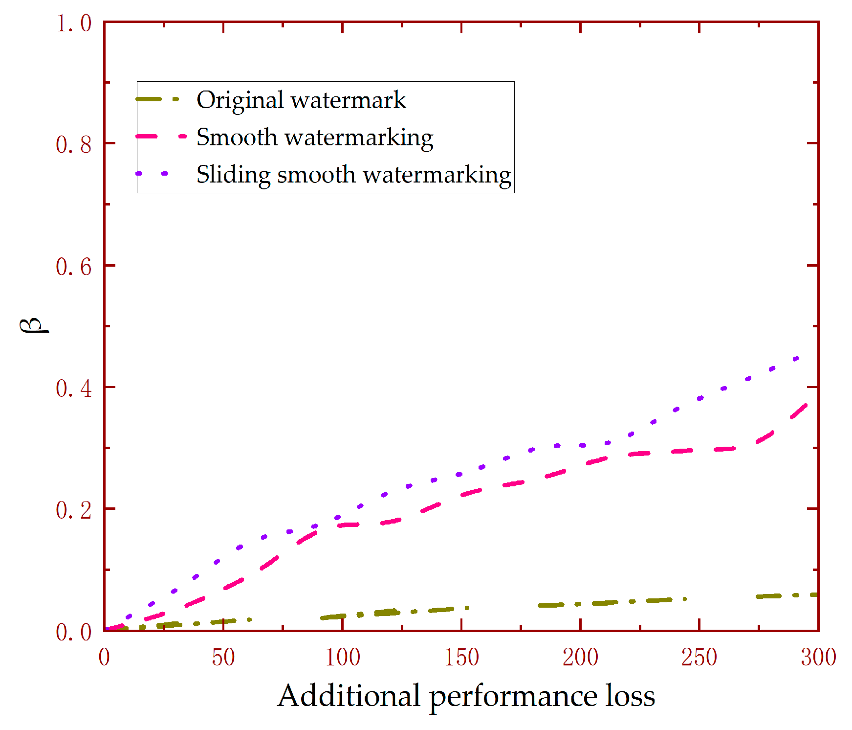
The sliding smooth watermarking method is introduced in the following. Two positive integer variables $u$ and $K_1$ are defined. $u$ indicates the number of smoothing segments, and $K_1$ indicates the size of the sliding window.

It is assumed that the original watermarking signal is divided into $u$ parts between two continuous signal points $\left({\xi }_k,\hspace{1em}{\xi }_{k+1}\right)$. A sliding window with the size $K_1$ is deployed to calculate the average of the first $K_1$ part.

For each $K_1$ part, there is an inner window with a variable size. The left side of the inner window overlaps the left side of the sliding window. The right side of the inner window moves one step to the right until it reaches the end of the sliding window. The mean of the first $K_1$ part is obtained by averaging the values derived from each moving step of the inner window. After moving the sliding window one step to the right, the second mean of the $K_1$ part is obtained. The sliding window continues to move right until it reaches the end of the original watermarking signal segment.

Ultimately, the final smooth signal is obtained by averaging the values derived from each moving step of the sliding window. Note that the smooth parameter $u$ and window size $K_1$ should satisfy the condition $u>K_1$, and the number of moving steps should be equal to $u-K_1+1$ $\left\{u,K_1 | u,K_1>0,u,K_1\in Z\right\}$.

A new sliding smooth watermarking signal $\Delta {\xi }_k$ is generated by performing the aforementioned process. In essence, the new watermarking signal is obtained by taking the sliding average of the sampling points of the original watermarking signal. The mathematical model of this new watermarking signal can be described as

$$\Delta {\xi }_k=\frac{1}{u-K_1+1}{\displaystyle \sum }_{m=1}^{u-K_1+1}\frac{1}{K_1}{\displaystyle \sum }_{i=m}^{K_1+m-1}\left[{\xi }_k+\left({\xi }_{k+1}-{\xi }_k\right)\frac{i}{n}\right],$$

(46)

It is worth noting that $u$ and $K_1$ can be freely designed. The statistical properties of the sliding smooth watermarking are

$$E\Delta {\xi }_k=E\left[\frac{1}{u-K_1+1}{\displaystyle \sum }_{m=1}^{u-K_1+1}\frac{1}{K_1}{\displaystyle \sum }_{i=m}^{K_1+m-1}\left[{\xi }_k+\left({\xi }_{k+1}-{\xi }_k\right)\frac{i}{u}\right]\right]=0$$

(47)

$$\begin{array}{ll}D\Delta {\xi }_k& =D\left[\frac{1}{u-K_1+1}{\displaystyle {\displaystyle \sum }_{m=1}^{u-K_1+1}}\frac{1}{K_1}{\displaystyle {\displaystyle \sum }_{i=m}^{K_1+m-1}}\left[{\xi }_k+\left({\xi }_{k+1}-{\xi }_k\right)\frac{i}{u}\right]\right]\\ & =E{\left(\frac{1}{u-K_1+1}{\displaystyle {\displaystyle \sum }_{m=1}^{u-K_1+1}}\frac{1}{K_1}{\displaystyle {\displaystyle \sum }_{i=m}^{K_1+m-1}}\left[{\xi }_k+\left({\xi }_{k+1}-{\xi }_k\right)\frac{i}{u}\right]\right)}^2\\ & =E\left[{\left(\frac{1}{u-K_1+1}{\displaystyle {\displaystyle \sum }_{m=1}^{u-K_1+1}}\left(\frac{{\xi }_k}{K_1}{\displaystyle {\displaystyle \sum }_{i=m}^{K_1+m-1}}\frac{u-i}{u}+\frac{{\xi }_{k+1}}{K_1}{\displaystyle {\displaystyle \sum }_{i=m}^{K_1+m-1}}\frac{i}{u}\right)\right)}^2\right]\\ & =E\left[{\left(\frac{1}{u-K_1+1}{\displaystyle {\displaystyle \sum }_{m=1}^{u-K_1+1}}\frac{{\xi }_k}{K_1}{\displaystyle {\displaystyle \sum }_{i=m}^{K_1+m-1}}\frac{u-i}{u}+\frac{1}{u-K_1+1}{\displaystyle {\displaystyle \sum }_{m=1}^{u-K_1+1}}\frac{{\xi }_{k+1}}{K_1}{\displaystyle {\displaystyle \sum }_{i=m}^{K_1+m-1}}\frac{i}{u}\right)}^2\right]\\ & =E\left[{\left(\frac{{\xi }_k}{u-K_1+1}{\displaystyle {\displaystyle \sum }_{m=1}^{u-K_1+1}}\frac{1}{K_1}{\displaystyle {\displaystyle \sum }_{i=m}^{K_1+m-1}}\frac{u-i}{u}+\frac{{\xi }_{k+1}}{u-K_1+1}{\displaystyle {\displaystyle \sum }_{m=1}^{u-K_1+1}}\frac{1}{K_1}{\displaystyle {\displaystyle \sum }_{i=m}^{K_1+m-1}}\frac{i}{u}\right)}^2\right]\\ & ={\left(\frac{1}{u-K_1+1}{\displaystyle {\displaystyle \sum }_{m=1}^{u-K_1+1}}\frac{1}{K_1}{\displaystyle {\displaystyle \sum }_{i=m}^{K_1+m-1}}\frac{u-i}{u}\right)}^2\mathsf{\Lambda }+{\left(\frac{1}{u-K_1+1}{\displaystyle {\displaystyle \sum }_{m=1}^{u-K_1+1}}\frac{1}{K_1}{\displaystyle {\displaystyle \sum }_{i=m}^{K_1+m-1}}\frac{i}{u}\right)}^2\mathsf{\Lambda }\end{array}$$

(48)

Let $D\Delta {\xi }_k=\mathsf{\Psi }\mathsf{\Lambda }$, where $\mathsf{\Psi }=\left(\gamma +\vartheta \right)$,$\gamma ={\left(\frac{1}{u-K_1+1}{\displaystyle {\displaystyle \sum }_{m=1}^{u-K_1+1}}\frac{1}{K_1}{\displaystyle {\displaystyle \sum }_{i=m}^{K_1+m-1}}\frac{u-i}{u}\right)}^2$, and $\vartheta ={\left(\frac{1}{u-K_1+1}{\displaystyle {\displaystyle \sum }_{m=1}^{u-K_1+1}}\frac{1}{K_1}{\displaystyle {\displaystyle \sum }_{i=m}^{K_1+m-1}}\frac{i}{u}\right)}^2$.

According to (35), the additional performance loss caused by the sliding smooth watermarking is

$$\Delta J^{\prime }\triangleq trace\left[\left(B^{T}SB+U\right)\mathsf{\Psi }\mathsf{\Lambda }\right],$$

(49)

$$\Delta J^{\prime }=\mathsf{\Psi }\Delta J.$$

(50)

Similar to the smooth watermarking signal, the additional performance loss caused by the sliding smooth watermarking signal can be less than that of the original watermarking signal by designing appropriate sliding smooth parameters.

5. Simulations

In this section, two simulation results are presented to demonstrate the effectiveness of the proposed watermarking smooth methods. Firstly, a numerical example of a process control plant is illustrated. Secondly, a double-tank system example is provided to test the effectiveness of the watermarking smooth methods.

5.1. Numerical Example

The model parameters of a discrete system are given as follows:

$$A=\left[\begin{array}{cc}0.8976& -0.0126\\ 0.01896& 0.9987\end{array}\right]$$

(51)

$$B=\left[\begin{array}{c}0.1896\\ 0.0193\end{array}\right]$$

(52)

$$C=\left[\begin{array}{cc}0& 0.0667\end{array}\right]$$

(53)

In the following, the effectiveness of the two watermarking smooth schemes proposed in this paper is analyzed. Additionally, we compare these methods with the watermark in [18] to illustrate the potential superiority. The control gain and Kalman filter gain then can be respectively designed as $L=\left[-1.1216,-0.8187\right]$ and $K=\left[0.1392,1.2406\right]$. The stability of the closed-loop system under replay attacks is guaranteed, as the eigenvalues of $A+BL$, $A-KCA$, $A$, and $\left(I-KC\right)\left(A+BL\right)$ all lie within the unit circle. In the following simulation, the parameters used in the smooth watermarking method and sliding smooth watermarking method are listed in

Table 1. The parameters used in the smooth watermarking method and sliding smooth watermarking method.

Method	Weight	Smooth Segment
smooth watermarking	$a=0.3$	$m=2$
	$b=0.2$	$n=2$
	$c=0.5$	$v=1$
method	step size	smooth segment
sliding smooth watermarking	$K_1=5$	$u=9$

.

As shown in Figure 2, the asymptotic detection rate $\beta$ is directly proportional to the variance $\mathsf{\Lambda }$ of the original watermarking signal for all three watermarks. However, the proposed smooth schemes have higher asymptotic detection rates compared with the watermark in [18] for a specified variance, $\mathsf{\Lambda }$. Looking at Figure 3, it is apparent that the asymptotic detection rate $\beta$ is proportional to the additional performance loss for all watermarking signals. However, the proposed smooth signals exhibit a higher asymptotic detection level compared with the watermark in [18] for the same additional performance loss $\Delta J$.

5.2. Double-Tank System

In this section, the effectiveness of the proposed watermarking smooth methods is demonstrated through a double-tank system. The double-tank system, as depicted in Figure 4, is a commonly used verification model in process control systems. The purpose of the system is to maintain the fluid level $h_2$ of tank 2 at a desired value by regulating inlet valve 1. The dynamic model of the double-tank system can be represented as

$$\Delta q_1-\Delta q_2=c_1\frac{d\Delta h_1}{dt},$$

(54)

$$\Delta q_2-\Delta q_3=c_2\frac{d\Delta h_2}{dt},$$

(55)

$$\Delta q_2=\left(\frac{\Delta h_1}{R_2}\right),$$

(56)

$$\Delta q_3=\left(\frac{\Delta h_2}{R_3}\right),$$

(57)

where $c_1$ and $c_2$ are the capacity coefficients. $R_1$, $R_2$, and $R_3$ represent the fluid resistance of the three valves, respectively. The transfer function of the double-tank system can be derived.

$$G(s)=\frac{h_2(s)}{q_1(s)}=\frac{K_0}{T_1{T}_2{s}^2+T_{2}s+T_{1}s+1},$$

(58)

where $T_1=c_1{R}_2$ is the time constant of tank 1, and $T_2=c_2{R}_3$ is the time constant of tank 2. $K_0=R_3$ means the magnification factor.

Let $c_1=33.33$, $c_2=0.2$, $R_2=9$, and $R_3=10$, and the state space expression of the double-tank system can be obtained.

$$\{\begin{array}{c}\dot{x}\left(t\right)=\left[\begin{array}{cc}-1.0033& -0.0033\\ 1.0000& 0\end{array}\right]x\left(t\right)+\left[\begin{array}{c}1\\ 0\end{array}\right]u\left(t\right)\\ y\left(t\right)=\left[\begin{array}{cc}0& 0.0333\end{array}\right]x\left(t\right)\end{array} ,$$

(59)

Given a sampling period of 0.2 s, the discrete model of the double-tank system can be represented as

$$\{\begin{array}{c}x\left(k+1\right)=\left[\begin{array}{cc}0.8181& -0.0006\\ 0.1812& 0.9999\end{array}\right]x\left(k\right)+\left[\begin{array}{c}0.1812\\ 0.0187\end{array}\right]u\left(k\right)\\ y\left(k\right)=\left[\begin{array}{cc}0& 0.0333\end{array}\right]x\left(k\right)\end{array},$$

(60)

In the following, the effectiveness of the two watermarking smooth schemes proposed in this paper is demonstrated. $W$ and $U$ in Equation (9) are set to be identity matrices. The controller and Kalman filter gains then can be respectively designed as $L=\left[-0.9006,-0.9018\right]$ and $K=\left[0.0502,1.1677\right]$. The stability of the closed-loop system under replay attacks is guaranteed according to the stability condition presented in Section 3.2. In the following simulation, the same parameters listed in Table 1 are used for the two watermarking smooth schemes.

The covariance matrices $Q$ and $R$ are equal to 0.8 times the identity matrix and identity matrix, respectively. According to (45), the additional performance loss of the smooth watermarking signal is $\Delta J^{\prime }=\frac{29}{50}\Delta J$. Similarly, the additional performance loss of the sliding smooth watermarking signal is $\Delta J^{\prime }=\frac{41}{81}\Delta J$. The additional performance losses of the proposed smooth signals are less than that of the watermark in [18]. Moreover, the additional performance loss of the sliding smooth method is lower compared with the smooth watermarking scheme. However, the sliding smooth method has a higher design and computational complexity.

As can be seen from Figure 5, the asymptotic detection rate $\beta$ is directly proportional to the variance $\mathsf{\Lambda }$ of the original watermarking signal for all three watermarks. However, the proposed smooth schemes have higher asymptotic detection rates compared with the watermark in [18] for a specified $\mathsf{\Lambda }$. Additionally, the sliding smooth watermarking signal exhibits a better asymptotic detection performance compared with the smooth watermarking signal.

As shown in Figure 6, the increase in the additional performance loss $\Delta J$ is proportional to the variance $\mathsf{\Lambda }$, which accords with the discussion in Section 3.3. However, the additional performance losses of the proposed smooth schemes are all smaller than that of the watermark in [18] for the same variance $\mathsf{\Lambda }$. In addition, the sliding smooth watermarking method possesses a lower performance loss compared with the smooth watermarking strategy.

From Figure 7, the asymptotic detection rate $\beta$ is proportional to the additional performance loss for every type of watermarking signal. However, the proposed smooth schemes exhibit a higher asymptotic detection level compared with the watermark in [18]. It is worth noting that the sliding smooth watermarking method demonstrates a superior asymptotic detection rate compared with the smooth watermarking strategy.

These numerical examples demonstrate that the watermarking scheme discussed in [18] exhibits lower performance when used to process control systems. The frequency should be reduced if it is to be used for process control systems. The smooth watermarking schemes proposed in this paper offer improved performance in terms of the additional performance loss and asymptotic detection rate. Additionally, the sliding smooth watermarking method outperforms the smooth watermarking scheme, although higher design and calculation complexity is required.

6. Conclusions

Two watermarking smooth methods, namely the smooth watermarking scheme and sliding smooth watermarking strategy, are proposed for detecting replay attacks in industrial process control systems. In light of these significant findings, we believe that our analysis may contribute to extending the original watermarking signal from dynamic systems to large-inertia process systems. The smooth watermarking signals significantly improve the detection of replay attacks in industrial process systems. These signals enhance the security of attack-sensitive systems, particularly nuclear power stations. Furthermore, these findings can also be applied to the field of fault diagnoses. Future studies will primarily focus on determining the optimal smooth parameters for a specified variance and an additional performance loss.

References

1. Naha, A.; Teixeira, A.; Ahlén, A.; Dey, S. Sequential detection of replay attacks. IEEE Trans. Autom. Control 2023, 68, 1941–1948. [Google Scholar] [CrossRef]
2. Sandberg, H.; Gupta, V.; Johansson, K.H. Secure networked control systems. Annu. Rev. Control Robot. Auton. Syst. 2021, 5, 445–464. [Google Scholar] [CrossRef]
3. Ding, D.R.; Han, Q.L.; Ge, X.H.; Wang, J. Secure state estimation and control of cyber-physical systems: A survey. IEEE Trans. Syst. Man Cybern. Syst. 2020, 51, 176–190. [Google Scholar] [CrossRef]
4. Zhang, H.; Liu, B.; Wu, H.Y. Smart grid cyber-physical attack and defense: A review. IEEE Access 2021, 9, 29641–29659. [Google Scholar] [CrossRef]
5. Inayat, U.; Zia, M.F.; Mahmood, S.; Berghout, T.; Benbouzid, M. Cybersecurity enhancement of smart grid: Attacks, methods, and prospects. Electronics 2022, 11, 3854. [Google Scholar] [CrossRef]
6. Bayou, L.; Espes, D.; Cuppens-boulahia, N.; Cuppens, F. Security issue of wirelesshart based SCADA systems. In Proceedings of the 10th International Conference on Risks and Security of Internet and Systems, Mytilene, Lesbos Island, Greece, 20–22 July 2015. [Google Scholar]
7. Smith, R.S. Covert misappropriation of networked control systems: Presenting a feedback structure. IEEE Control Syst. Mag. 2015, 35, 82–92. [Google Scholar]
8. Whitehead, D.E.; Owens, K.; Gammel, D.; Smith, J. Ukraine cyber-induced power outage: Analysis and practical mitigation strategies. In Proceedings of the 70th Annual Conference for Protective Relay Engineers, College Station, TX, USA, 3–6 April 2017. [Google Scholar]
9. Hemsley, K.E.; Fisher, E. History of Industrial Control System Cyber Incidents; No. INL/CON-18-44411-Rev002; Idaho National Lab: Idaho Falls, ID, USA, 31 December 2018.
10. Wang, A.M.; Fei, M.R.; Song, Y.; Peng, C.; Du, D.J.; Sun, Q. Secure adaptive event-triggered control for cyber–physical power systems under denial-of-service attacks. IEEE Trans. Cybern. 2023. [Google Scholar] [CrossRef] [PubMed]
11. Li, T.X.; Wang, Z.D.; Zou, L.; Chen, B.; Yu, L. A dynamic encryption–decryption scheme for replay attack detection in cyber–physical systems. Automatica 2023, 151, 110926. [Google Scholar] [CrossRef]
12. Kashima, K.; Inoue, D. Replay attack detection in control systems with quantized signals. In Proceedings of the 2015 European Control Conference, Linz, Austria, 15–17 July 2015. [Google Scholar]
13. Hosseinzadeh, M.; Sinopoli, B.; Garone, E. Feasibility and detection of replay attack in networked constrained cyber-physical systems. In Proceedings of the 57th Annual Allerton Conference on Communication, Control, and Computing, Monticello, IL, USA, 24–27 September 2019. [Google Scholar]
14. Yaseen, A.A.; Bayart, M. Attack-Tolerant networked control system based on the deception for the cyber-attacks. In Proceedings of the 2015 World Congress on Industrial Control Systems Security, London, UK, 14–16 December 2015. [Google Scholar]
15. Mo, Y.L.; Sinopoli, B. Secure control against replay attacks. In Proceedings of the 47th Annual Allerton Conference on Communication, Control, and Computing, Monticello, IL, USA, 30 September–2 October 2009. [Google Scholar]
16. Ferrari, R.M.; Teixeira, A.M. A switching multiplicative watermarking scheme for detection of stealthy cyber-attacks. IEEE Trans. Autom. Control 2020, 66, 2558–2573. [Google Scholar] [CrossRef]
17. Du, D.J.; Zhang, C.D.; Li, X.; Fei, M.R.; Zhou, H.Y. Attack detection for networked control systems using event-triggered dynamic watermarking. IEEE Trans. Ind. Inform. 2022, 19, 351–361. [Google Scholar] [CrossRef]
18. Mo, Y.L.; Weerakkody, S.; Sinopoli, B. Physical authentication of control systems designing watermarked control inputs to detect counterfeit sensor outputs. IEEE Control Syst. Mag. 2015, 35, 93–109. [Google Scholar]
19. Satchidanandan, B.; Kumar, P.R. Dynamic watermarking: Active defense of networked cyber-physical systems. Proc. IEEE 2017, 105, 219–240. [Google Scholar] [CrossRef]
20. Zhao, Y.; Smidts, C. A control-theoretic approach to detecting and distinguishing replay attacks from other anomalies in nuclear power plants. Prog. Nucl. Energy 2020, 123, 103315. [Google Scholar] [CrossRef]
21. Huang, T.; Satchidanandan, B.; Kumar, P.R.; Xie, L. An online detection framework for cyber attacks on automatic generation control. IEEE Trans. Power Syst. 2018, 33, 6816–6827. [Google Scholar] [CrossRef]
22. Fang, C.R.; Qi, Y.F.; Cheng, P.; Zheng, W.X. Cost-effective watermark-based detector for replay attacks on cyber-physical systems. In Proceedings of the 11th Asian Control Conference, Gold Coast, QLD, Australia, 17–20 December 2017. [Google Scholar]
23. Liu, H.X.; Yan, J.Q.; Mo, Y.L.; Johansson, K.H. An on-line design of physical watermarks. In Proceedings of the 2018 IEEE Conference on Decision and Control, Miami, FL, USA, 17–19 December 2018. [Google Scholar]
24. Porter, M.; Hespanhol, P.; Aswani, A.; Johnson-Roberson, M.; Vasudevan, R. Detecting generalized replay attacks via time-varying dynamic watermarking. IEEE Trans. Autom. Control 2020, 66, 3502–3517. [Google Scholar] [CrossRef]
25. Miao, F.; Pajic, M.; Pappas, G.J. Stochastic game approach for replay attack detection. In Proceedings of the 52nd IEEE Conference on Decision and Control, Firenze, Italy, 10–13 December 2013. [Google Scholar]
26. Fang, C.R.; Qi, Y.F.; Cheng, P.; Zheng, W.X. Optimal periodic watermarking schedule for replay attack detection in cyber-physical systems. Automatica 2020, 112, l08698. [Google Scholar] [CrossRef]
27. Forment Navarro, A. Security Analysis of a Wireless Quadruple Tank Control System. Master’s Thesis, KTH Royal Institute of Technology, Stockholm, Sweden, May 2011. [Google Scholar]
Figure 1. Control system with replay attacks and watermarking signal.
Electronics 12 03812 g001
Figure 2. Comparisons of the asymptotic detection rates with different Λ .
Electronics 12 03812 g002
Figure 3. Comparisons of the asymptotic detection rates with different additional performance losses.
Electronics 12 03812 g003
Figure 4. Double-tank control system.
Electronics 12 03812 g004
Figure 5. Comparisons of the asymptotic detection rateswith different Λ for the double-tank system.
Electronics 12 03812 g005
Figure 6. Comparisons of the additional performance losses with different Λ .
Electronics 12 03812 g006
Figure 7. Comparisons of the asymptotic detection rates with different additional performance losses for the double-tank system.
Electronics 12 03812 g007