Abstract
Dispatching and cooperative trajectory planning for multiple autonomous forklifts in a warehouse is a widely applied research topic. The conventional methods in this domain regard dispatching and planning as isolated procedures, which render the overall motion quality of the forklift team imperfect. The dispatching and planning problems should be considered simultaneously to achieve optimal cooperative trajectories. However, this approach renders a large-scale nonconvex problem, which is extremely difficult to solve in real time. A joint dispatching and planning method is proposed to balance solution quality and speed. The proposed method is characterized by its fast runtime, light computational burden, and high solution quality. In particular, the candidate goals of each forklift are enumerated. Each candidate dispatch solution is measured after concrete trajectories are generated via an improved hybrid A* search algorithm, which is incorporated with an artificial neural network to improve the cost evaluation process. The proposed joint dispatching and planning method is computationally cheap, kinematically feasible, avoids collisions with obstacles/forklifts, and finds the global optimum quickly. The presented motion planning strategy demonstrates that the integration of a neural network with the dispatching approach leads to a warehouse filling/emptying mission completion time that is 2% shorter than the most efficient strategy lacking machine-learning integration. Notably, the mission completion times across these strategies vary by approximately 15%.
1. Introduction
The increasing demands in the logistics industry all over the world have driven researchers and engineers to focus on developing intelligent transportation systems aimed at enhancing logistics efficiency [1,2]. One prominent application in this domain is unmanned warehouse systems [3]. As a typical component in an unmanned warehouse, an autonomous forklift transports parcels more efficiently than one driven manually because the former does not induce objective mistakes such as fatigue, anxiety, impatience, or anger [4]. Multiple autonomous forklifts should work together when the delivery burden is heavy [5]. Deploying multiple autonomous forklifts enhances delivery efficiency if the inter-forklift cooperation potential can be maximized. The typical modules that influence delivery efficiency include delivery task dispatch [6], cooperative trajectory planning [7,8], and control [9]. This paper is focused on the dispatching and cooperative trajectory planning schemes.
1.1. Related Work
1.1.1. Dispatching Methods for Multiple Forklifts
A complete multi-forklift delivery planning system consists of two functions: delivery task dispatch and cooperative trajectory planning. Before cooperative trajectory planning, the goal point of each forklift is assigned in the dispatching phase [10]. Weidinger et al. [6] proposed a metaheuristic-based method in which assignment candidates are pruned a priori to facilitate the solution process [11]. A similar idea was proposed by Zhang et al. [12] to dispatch multiple automated guided vehicles (AGVs) in a matrix manufacturing workshop. However, both methods run slowly; thus, they cannot meet the real-time computation demand in a warehouse [6,12]. Lin et al. built a multi-AGV dispatching system via network structure together with simplex decision variables; in this system, an evolutionary algorithm minimizes the completion time of all AGVs in a formulated network optimization problem. However, References [6,12,13] shared a common limitation of assuming a uniform speed for AGVs. Moreover, the inter-vehicle collision avoidance problem is reduced to an oversimplified constraint, ensuring solely nonoverlapping time intervals per stopover.
Furthermore, recent studies have focused on the task integration of one AGV instead of considering how multiple AGVs cooperatively operate within the confined area. Bao et al. [14] proposed a heuristic method based on an auction strategy for a multi-AGV task dispatch scheme considering complex factors (such as pod repositioning). The concerned dispatch scheme is inherently an optimization problem with complex cost terms and constraints facilitated by the proposed auction strategy. Lee et al. [15] proposed a two-stage dispatching method. In particular, the first stage deals coarsely with the delivery efficiency and delivery flow balance by solving a bi-objective optimization problem. The result indicates how the parcels to be picked can be clustered. At stage 2, vehicles are dispatched to complete the clustered missions. Dividing the original scheme into two stages largely reduces the number of dispatch candidates without losing the optimum. Machine-learning-based dispatching methods have also been proposed [16]. The formulated reward functions efficiently simplify the dispatch scheme, particularly when complex factors are considered [17,18]. However, few vehicle kinematics is considered in [14,15], and the dispatching phase is fully separated from the trajectory planning strategy. This approach results in difficulties in maximizing overall delivery efficiency.
1.1.2. Cooperative Trajectory Planning Methods for Multiple Forklifts
Cooperative trajectory planning follows the aforementioned dispatching phase. The prevalent cooperative trajectory planners are based on model predictive control [19], which is highlighted by its fast feature while strictly satisfying safety-related constraints. The artificial potential field method is similarly widely applied in trajectory planning, but it may encounter difficulty finding paths through narrow passages [20].
Ma et al. [21] converted constrained time-varying nonlinear programming problems to general unconstrained optimization problems by properly designing a penalty function. Thereafter, a particle swarm optimization method was employed to plan the motion of multiple robots sequentially in a double warehouse with two elevators. However, the optimization phase, along with other methods based on optimization, can significantly increase the computational burden [22,23,24], which can be reduced by forming model-based paths because warehouses are generally structured.
Yang et al. [1] proposed a strategy in which a time-varying dynamic evaluation function is formed based on a network congestion diffusion model to quantify the degree of road congestion. Hereafter, an improved A* search algorithm and a time window algorithm were combined as a hierarchical planning method to search the idle path and avoid collisions. A path planning framework was designed by Zhou et al. [25] to simultaneously reduce the cost of operation and the path for AGVs in airport parcel loading scenarios. An ant colony optimization method was used to optimize the parcel pickup sequencing by ignoring other moving vehicles, while Dijkstra’s algorithm was employed to determine the shortest route of each AGV. Zacharia et al. developed a joint routing and motion planning method for AGVs that addresses uncertainties in demands and travel times. Their approach combines a scheduler for updating destination resources during navigation and integrates a fuzzy-based genetic algorithm with A* search to handle capacity and distance variations [26]. Nonetheless, the vehicle kinematics considered in [1,25,26] remain oversimplified for industrial use even in the trajectory planning phase.
In other studies, the paths of vehicles were assumed to be predefined, and only the longitude trajectories were investigated. Kneissl et al. [27] formulated a method in which potential collision zones are continuously detected. Moreover, the right-of-way is granted to the first arriving vehicle while all the other vehicles involved stop and wait. Dresner et al. proposed confronting the analogous problem of conflict zones with a reservation-based system; in this system, vehicles request and receive time slots from the intersection while they pass [28]. Similarly, a discrete-event logic, which is comparable with a conventional right-handed bidirectional traffic system, was designed by Guney et al. [29] to handle the priorities of the AGVs in a warehouse dynamically. Thus, the need for computationally demanding heuristic searches is eliminated to ease strategy implementation in real-life industrial applications. Furthermore, Digani et al. [30] proposed an obstacle-free path generation method to deal with local deviations from the predetermined path. In the proposed method, new paths are generated via polar spline curves. However, the aisles in a warehouse cannot be fully exploited when certain traffic laws in [27,28,29,30] are strictly enforced.
1.1.3. Joint Dispatching and Planning Methods for Multiple Forklifts
Most of the existing dispatching studies, e.g., [6,10,11,12,13,14,15,16,17,18], cannot accurately evaluate the candidate choices, possibly preventing the downstream planning module from achieving global optimality [1,21,22,23,24,25,26,27,28,29,30]. Thus, combining the dispatching and planning phases is naturally considered. The multi-agent path finding (MAPF) problem in its classical form is an effective approach for simplifying complex warehouse scenarios and facilitating cooperative solutions for dispatching and planning. In the MAPF problem, time is discretized into steps, allowing vehicles to either move or wait during each step [31]. Consequently, it becomes challenging to plan trajectories for vehicles with varying velocities or based on specific kinematic constraints. To address this limitation, researchers have explored extensions of the MAPF problem to accommodate such complexities. Among those extensions, Zhang et al. [32] designed a joint strategy to deal with an automatic valet parking system, in which a travel-distance-related reward function combined with a deep reinforcement learning technique was used to allocate the target parking spaces. The parking lot was segmented into local regions, and a rule-based right-of-way assignment strategy was applied to solve collisions and deadlocks. A simplified trajectory planning algorithm based on the car-following model [33] served as a tool to solve the trajectories of multiple AGVs when no potential collision was involved. A similar strategy was proposed by Lee et al. [34] for a supply-chain-connected warehouse. In their work, a cloud-based semiautomatic warehouse management system assigns tasks to mobile robots to optimize resource allocation. A robot control system executes an improved A* search algorithm to generate the path of each AGV. Then, potential collisions, named stay-on, head-on, and cross-conflict, are identified and solved by following certain priority-based rules. Redispatchment of the AGV with low priority is triggered as the conflict cannot be prevented by those basic rules.
With regard to joint strategies, the studies above [32,34] can deal with large-scale AGV-based scenarios. However, these studies were concerned with vehicles possessing the simple kinematics of unicycle (differential-drive) robots [35] and generally focused on the construction of maneuverable systems, ignoring the overall optimal solutions concerning warehouse operations. Furthermore, during the trajectory planning phase, they initially planned only the paths and ignored other moving obstacles. Such considerations substantially reduce the risk of collisions and simplify the evaluation of the traveling difficulties pertaining to one potential task relative to the corresponding traveling distance. In other words, it remains unknown the specific trajectory pertaining to each AGV as the jointed strategy is finished, and this trajectory is dependent on local scenes when conflict zones are involved. Thus, the results become unreliable when such strategies are applied to a warehouse of automated forklifts with complex kinematics. As a conclusion of this subsection, it deserves to develop a joint dispatching and planning method to balance the forks’ motion quality and reaction speed in an unmanned warehouse.
1.2. Motivations
This study aims to substantially improve the efficiency of cooperative operations among multiple autonomous forklifts by seamlessly integrating the dispatching and cooperative trajectory planning phases. Our primary objective is to address the limitations of existing dispatching methods, which often overlook low-level forklift kinematic capability. To overcome this challenge, we opt for the implementation of a graph search process in this phase. Moreover, to ensure a robust solution that avoids getting trapped in local optima, we chose to incorporate a machine-learning-based technique. In the trajectory planning phase, we recognize that optimization-based methods are computationally expensive. As such, our secondary objective is to develop an alternative search algorithm that employs a model-based approach. This algorithm is designed to be both velocity-aware and sequentially solvable, striking a balance between accuracy and computational efficiency.
1.3. Contributions
The core contribution of this paper is the proposal of a joint framework, which is promising to reduce the computational burden because all formulations involved are explicitly expressed. Concretely, the dispatching stage can enhance the multi-vehicle task solution quality because it considers the future trajectory pertaining to each forklift. Moreover, the kinematically feasible and safe trajectory of each forklift can be quickly generated through our proposed method at the trajectory planning stage, due to the removal of optimization-based methods.
1.4. Organization
In the rest of this paper, Section 2 formulates the in-warehouse delivery problem. Section 3 provides the score-based dispatching technique, in which ANN is applied to avoid deadlocks in evaluating the cost of each candidate dispatching option. Section 4 introduces the trajectory planning method, namely a model-based velocity-aware hybrid A* search algorithm. Section 5 integrates the two aforementioned methods to develop a joint dispatching and cooperative trajectory planning framework, followed by Section 6, where comparative simulation results are present. Conclusions are drawn in Section 7, finally.
2. Problem Statement
Forklifts are used to deliver goods between fixed picking stations and predetermined shelf areas during delivery tasks in warehouses. The passages are generally designed to be narrow, and they merely allow turning maneuvers with a minimum radius and the passing of only two vehicles. Hence, conflicts arise when multiple forklifts cooperatively operate within a single warehouse.
Within one subtask during the filling of one warehouse, there are two stages: first, the initial pose and the final one should be assigned to one forklift as the dispatching stage; second, the trajectory planning stage generates a trajectory by avoiding collisions with any static or moving objects and satisfying the vehicle kinematics.
2.1. Warehouse Layout
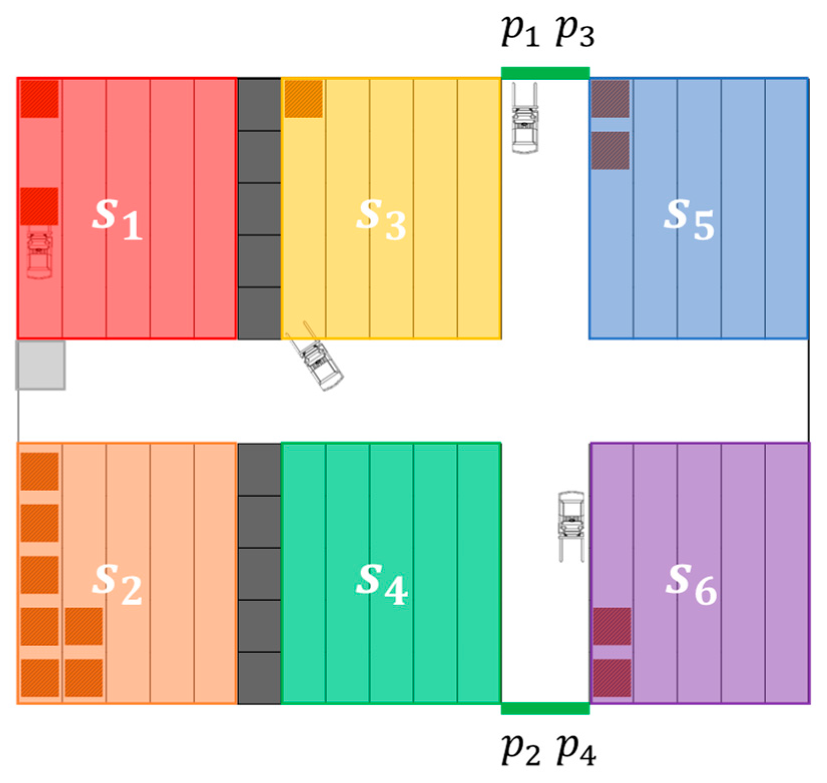
A typical small warehouse layout is schematized in Figure 1. In this warehouse, six separated shelf clusters, denoted as (), are placed and provide areas to store goods. Continuous lines indicate shelf walls, through which forklifts cannot move. Two firewalls, represented by rows of grey squares, are present between shelf cluster and as well as cluster and . Meanwhile, four picking stations, marked with slender solid rectangles and (), are located in both extremities of the vertical and wide passage in Figure 1. Four forklifts can enter the passage of each row of the shelf clusters, as long as neither stored stacks nor other vehicles block the route.

Figure 1.
Schematic of a warehouse layout.
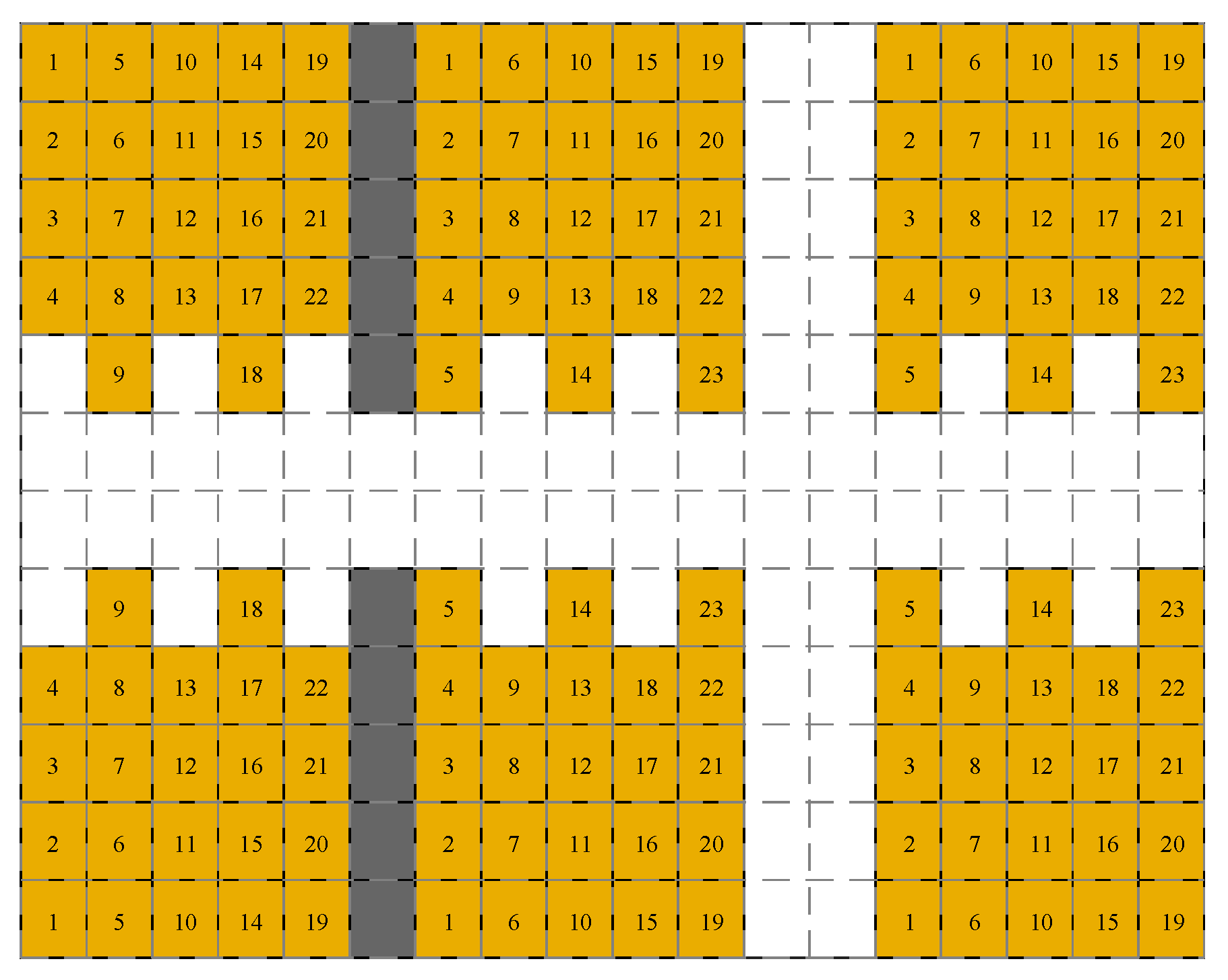
As presented in Figure 2, each shelf cluster has the capacity to accommodate varying numbers of goods stacks with strategically positioned notches in the arrangement designed to suit forklift kinematics during turns. This aspect will be elaborated on in Section 2.2. Each stack is marked with a number in Figure 2 to represent the order in which a shelf cluster can be filled. The shelf filling state and the vehicle state can be effectively expressed by noting the covered grids when the warehouse is divided by the squares outlined by grey dashed lines in Figure 2. In addition, when one forklift is unloading goods within a shelf cluster, its fork side should point to the stack position (cf. upper left forklift schematic and within shelf cluster in Figure 1). Similarly, when one forklift is picking goods at a picking station, the fork side should point to the station position (cf. upper forklift schematic and picking station in Figure 1).
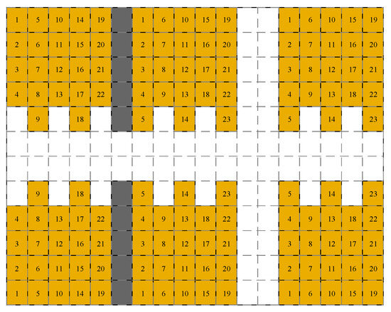
Figure 2.
Filling sequence pertaining to each shelf cluster.
2.2. Kinematics of a Forklift Vehicle
As reported in Figure 3, a forklift can be described as a front-steering vehicle if the fork part of the vehicle is treated as the rear side. The corresponding kinematic formulas write:
where is time; , located at coordinate (, ), indicates the mid-point of the rear wheel axis; and , , , , and respectively denote the orientation angle, linear velocity pertaining to point , acceleration, steering angle of the front wheels, and steering rate. Furthermore, stands for the wheelbase length, denotes the rear overhang length, refers to the front overhang length, and is the car width. Given that the initial values as well as and are provided, the state variables can be calculated through integration over the dynamic process.
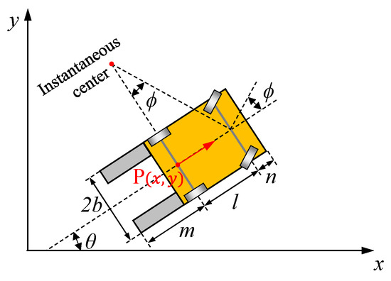
Figure 3.
Parametric notations related to vehicle size and kinematics.
Meanwhile, a few boundaries are imposed on the state profiles over the entire simulation period throughout all dynamic maneuvers:
where , , , and respectively indicate the upper limits of the corresponding variables.
3. ANN-Combined Score-Based Dispatching Approach
Filling a warehouse in an orderly manner requires several forklifts to perform multiple deliveries and return subtasks. In the current work, subtasks are assigned to different vehicles sequentially. With regard to such subtasks, selecting which vehicle will be used to plan the new trajectory and determining which goal coordinates the forklift is going to should comprise the fundamental initialization. Therefore, a dispatching system is necessary to solve these problems.
The dispatching approach (cf. Algorithm 1) utilizes the planned trajectories of all vehicles, along with map information , and vector representing filled stacks for different clusters, as its inputs. The core of this approach lies within a while loop, wherein the potential subtask undergoes iterative updates (with a preset maximum iteration number ) until it reaches an optimal state, as defined by the proposed method.
Outside of the loop, the function sorts all vehicles based on , arranging them in ascending order from first to last. This sorting process generates a ranking vector consisting of four vehicle indices. If , indicating a failure in the trajectory search between at instant and , the corresponding vehicle is repositioned at the end in and flagged as having been selected as . In the loop, the algorithm is divided into two parts. The first one (lines 4 to 13) concerns the selection of the current investigated vehicle with an index of , and the second part (lines 14 to 30), featuring a scoring system combined with the results of an ANN method, determines the goal coordinate for the current subtask. Notably, Algorithm 1 is applied when the ANN correction system, which is elaborated on in Section 3.2, is enforced.
| Algorithm 1: ANN combined score-based dispatching algorithm |
|
3.1. Vehicle Selection and Initial Pose of a New Subtask
The function selects the vehicle, ranking the first one as , and sets , which is the initial instant of the trajectory to be planned, as the ending instant of the last trajectory pertaining to . Failure may occur in the determination of the new trajectory for the fork in the new subtask because other forklifts may block the only corresponding route for a considerable time. Under such circumstances, a flag variable is set to 1, and all vehicles in are checked to see if they have been selected as once for the current subtask by . The function is then utilized. In this function, the first motion-finished vehicle is discarded, and the other forklifts are subsequently selected in turn as on the basis of the rankings in until the trajectory can be formed. Furthermore, no trajectory can be successfully planned for all forklifts at certain moments. In this case, is applied, in which the vehicle that ranks last in is selected, and the of the new trajectory is postponed for a fixed time length of relative to the end of the last subtask for vehicle . The vehicle final stopping pose is set as the initial pose of the new subtask by function .
3.2. Scoring System
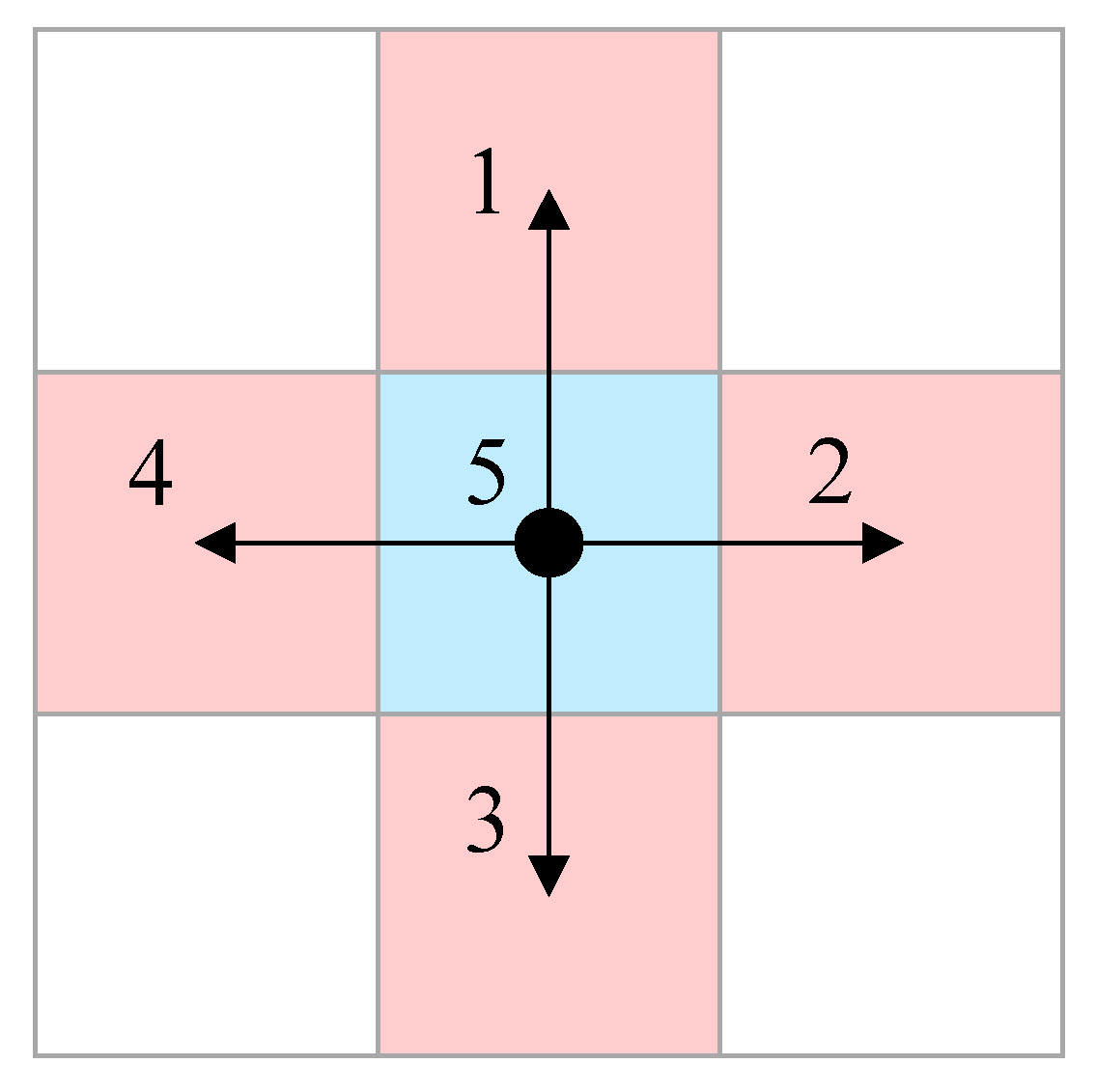
A scoring system is applied to decide the goal coordinate of the new subtask. First, the function is initially employed to ascertain whether the planned trajectory involves heading to clusters or returning. The functions and are then applied separately depending on whether the goal is a rack cluster or a picking station. In both functions, the grid networks, outlined by light colors in Figure 2, indicate the nodes used to define the location of a vehicle and stacks. The resolution of such nodes is purposely reduced with the aim of lowering computation costs. Given that the nodes are defined, a time dimension involved preliminary A* search algorithm, whose expansion manner is presented in Figure 4, is used to generate preliminary trajectories that link the starting pose at instant to each potential target coordinate. Five patterns in total for this search algorithm are applied to vaguely indicate the possible maneuvers a vehicle could perform. In particular, manner 5 in Figure 4 expands only in the time dimension, representing the stopping condition of a virtual forklift. The time consumed derived from this algorithm for a virtual vehicle represented by one node is then applied as a parameter to evaluate the difficulty grades of reaching different goal poses. Other vehicles and walls are treated as obstacles during the search. Notably, the orientation angles for the initial and final poses are not required to be determined in such a system. Thus, is not considered a dimension in this search for the sake of calculation simplification.
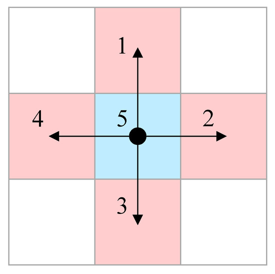
Figure 4.
Expansion manner of the preliminary hybrid A* search.
In the function , the function is applied to evaluate the scores pertaining to different target stack locations (cf. Figure 1) when a subtask with one stack as the goal is considered. It writes:·
where denotes the number of stacks to be filled/emptied in the target shelf cluster in order to balance the warehouse filling/emptying mission in different clusters. stands for the approximate difficulty to reach different goal coordinates in shelf cluster . is a negative constant applied when the goal in practice is not reachable. indicates time length . counts the time units during which other vehicles occupy the shelf entrance node (cf. the grey grid for the upper left forklift in in Figure 1) of the goal pose within a fixed time length after the virtual vehicle entering the rack passage. The reason is added as a parameter is that, in practice, the availability of the above-mentioned node is critical during the planning of the final trajectory that considers kinematics. is a function of the time length consumed to arrive at the target in this preliminary search. Notably, this function is built to normalize the results for different shelf clusters because shelf clusters and are far from the picking stations, and delivering goods to these locations consumes much time. Furthermore, a negative constant is assigned to when the target cannot be reached through the search within a predefined maximum iteration number . Meanwhile, , ,…, are calibration parameters. Among these, a substantial weighting coefficient, , is allocated to regulate the stacks filled in each shelf cluster; aiming for balance, , , , and are designed to quantitatively assess scores with respect to time considerations. If is derived within , the vehicle kinematics-considered trajectory is difficult to find. Thus, the flag variable is set to 1 in the initialization cycle, where ANN is not enforced, and should be reassigned.
Similarly, in the function , only the time consumed with respect to different picking stations (cf. Figure 1) in the A* search is used in the evaluation of , which is expressed as:
When ANN is not enforced, the potential targets are initially scored solely by means of Equations (3) and (4). The greater the functions to be evaluated are, the greater the likelihood of subsequent trajectory planning is and the faster the entire warehouse can be filled. In this case, and are selected as the goal poses for delivery and return subtasks, respectively.
3.3. ANN Correction Method
The function is employed to refine goal score evaluations through a multilayer perceptron (MLP) network, which is elaborated upon as follows.
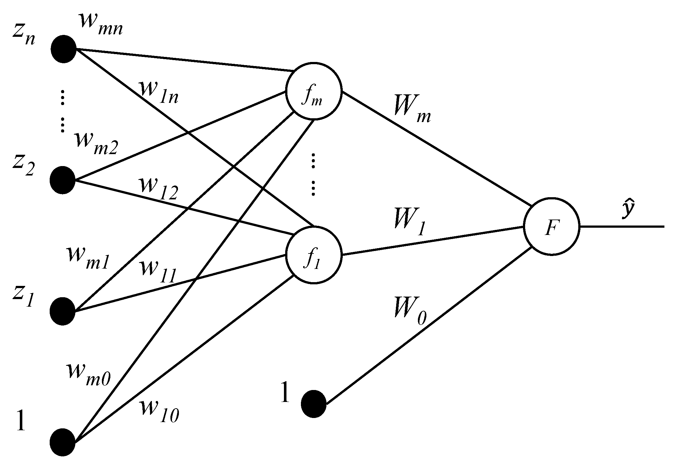
Figure 5 presents a typical MLP network of ANN with one hidden layer. Mathematically, with the trajectory planning states as known variables, the MLP network of the type reported in Figure 5 can be expanded step by step as follows:
where and denote the weights assigned to the connection of the neurons. and are linked to the bias, whose values are simply the constant 1.
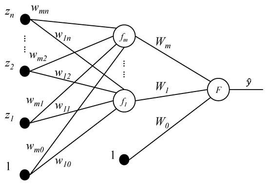
Figure 5.
Schematic of an MLP network.
The ANN correction in the current study is designed for the scoring system for the goal pose determination of delivery subtasks. In the initialization phase of the ANN correction system, excluding the filling balance parameter of in Equation (3), respectively denote the base values of the output elements in (cf. in Figure 5) for six MLP networks. Among the six elements, the one whose corresponding pose is selected as the target for vehicle kinematics-considered trajectory planning is further fixed based on the corresponding trajectory variables. The values of the other elements remain as unchanged as the results in Equation (3). Suppose that is the shelf cluster investigated within a subtask. Given that the base value is derived with Equation (3), if that corresponds to is selected as the goal to determine the trajectory, then the trajectory with the goal of will be planned, and the corresponding element in will be derived with Equation (6) as follows:
where is the ending instant of the trajectory, stands for the average value of the time length pertaining to all previously derived trajectories, is a calibrated constant intended to balance , and the latter solely accounts for time consumed to reach a goal without factoring in the distance covered. and are respectively used to normalize the difference in distances corresponding to various shelf clusters and the expected moving time period of each subtask.
Similar to the parameter in Equation (3), the inputs (cf. in Figure 5) of the ANN system are the number of stacks filled within each shelf cluster. A vector with six elements }, which correspond to six shelf clusters , is used. Suppose that is considered, it can be formulated as
The integers other than 0 can represent the filling states of the shelf clusters, which are associated with the currently moving forklifts. The vehicle motion states are also observed. This input of the MLP network vaguely provides information associated with the possible area the vehicles may be located in, given that each shelf cluster should be filled by following certain orders. Furthermore, at least two shelf clusters are not connected to any subtask because only four forklifts in the warehouse are employed. Evidently, these shelf clusters have no impact on the trajectory planning, and this situation is in line with the circumstances, where the investigated shelf group is filled. Thus, 0 is assigned to in this case.
As the number of hidden neurons is set to 12 according to an empirical technique [36], the MLP system used to score shelf cluster can be expressed in the form of Equation (5) as
The Levenberg-Marquardt method is then used to train the MLP and the values assigned to the elements of and .
In the following warehouse filling cycles and the final dispatching system, the scoring system described in Equation (3) is replaced by the expression below to determine the optimal goal pose for vehicle . Equation (9) is the final scoring equation of the discussed dispatching system, wherein and act as the calibration constants. These constants are determined via a trial-and-error approach to yield results. The MLP contributes without excessively disrupting performance concerning warehouse filling/emptying time.
After the initialization cycle of warehouse filling (referring to Figure 6), the training process can continue until cycles are finished. In the following cycles, the MLP has already been established depending on the data pertaining to the previous cycles, and the saved values of and are used to estimate the values via Equation (8). Therefore, the base values of the MLP outputs are replaced by in Equation (9) when shelf cluster is considered. The expression of the corresponding element in for the following cycles writes:
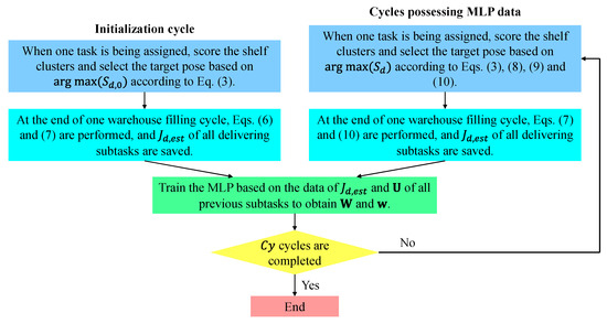
Figure 6.
Flowchart of MLP training.
3.4. Final Pose Selection
The final pose of each subtask is determined using the function. For subtasks with the purpose of delivery, the destination coordinate is chosen based on the criterion; for return subtasks, the coordinate corresponding to is selected. Finally, the corresponding information should be added to complete the destination pose.
4. Improved Hybrid A* Search Algorithm
Hybrid A* algorithm [37] is an extension of the conventional 2D A* search algorithm due to its consideration of kinematics during node expansions over time. Different from the original hybrid A* search, the velocity variation is considered, and the node expansion manner is determined based on action purposes in the algorithm (cf. Algorithm 2) applied in this study. Furthermore, this improved heuristic method directly determines trajectory details throughout a subtask without an optimization stage.
Algorithm 2 is used to expand a parent node () in one manner through the improved hybrid A* search with the target of . Focusing on the motion of one vehicle, is used to store the data pertaining to all nodes (), which has been explored and can be further expanded. The information contains the corresponding parent nodes, expansion manner (cf. Section 4.1), time expansion data (cf. Section 4.2), and costs (cf. Section 4.4). On the contrary, the node () cannot be expanded anymore and is stored in . Furthermore, the function is discussed in Section 4.3. In addition, the function is used to add a node with its affiliating data into or .
| Algorithm 2: Improved hybrid A* search algorithm |
|
4.1. Node Expansion Method
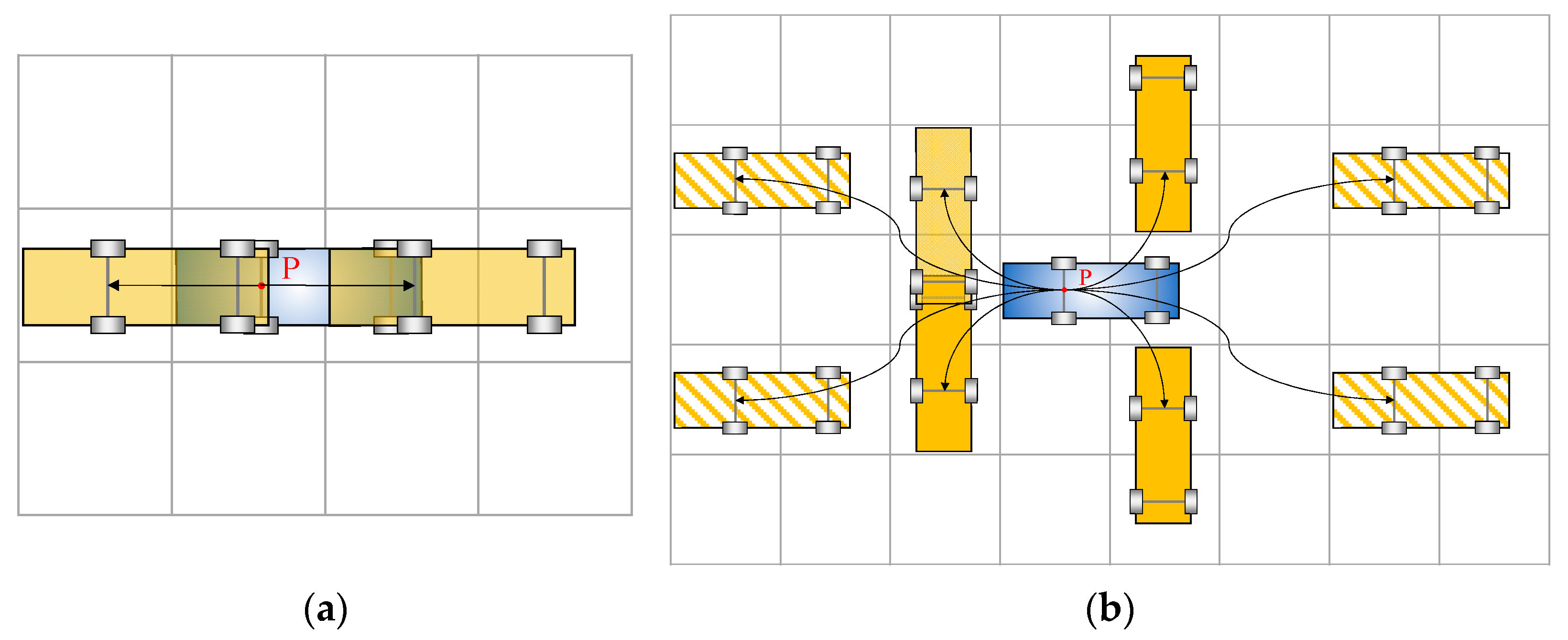
This section elaborates on the various possible expansion manners denoted as , with each individual possibility represented by . The drivable area is initially mapped with the above-discussed grid networks (cf. Figure 2). The dimensions of the grid should be skillfully coupled with the size of the vehicle, with the aim of reducing occupied cells during a certain action and enhancing the utility rate of the space. The case demonstrated in Figure 7 is a well-designed example. In this case, one vehicle covers two grid cells. Thus, on a 2D space domain, the orientation angle involved in forklift movements can be easily described. In addition, through one maneuver, the vehicle body occupies a small number of grids. This can reduce the possibility of interference with other forklifts during motion planning.
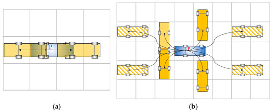
Figure 7.
Node expansion manners of improved hybrid A* algorithm: (a) Stopping and going straight; (b) lane changing and turning.
As reported in Figure 7a,b, the nodes expanding manners in the space domain can be divided into eleven patterns, which are summarized as four categories covering all possible maneuvers a forklift may intend to conduct. These include stopping, going straight (cf. semitransparent solid rectangles in Figure 7a), lane changing (cf. rectangles with diagonal stripes in Figure 7b), and turning (cf. solid rectangles in Figure 7b).
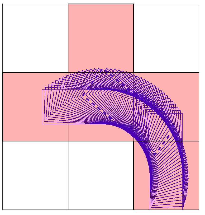
As far as the expanding manners are concerned, when remains 0, one vehicle stops. As is other than 0 with steering angle , one fork can go or reverse straight. Figure 8 demonstrates one modeled forklift path depicted by consecutive outlines, when the vehicle goes upward and turns to the left from the right lower side to the center left. Through this maneuver, is varied to gain an identical final location relative to grids as the initial state, despite the change of in . Under such circumstances, the consecutive motions can be easily established. Meanwhile, the modeled maneuver of reverse turning to the left can also be noted in Figure 8, when the initial and final body outlines are exchanged.
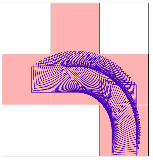
Figure 8.
Path of turning.
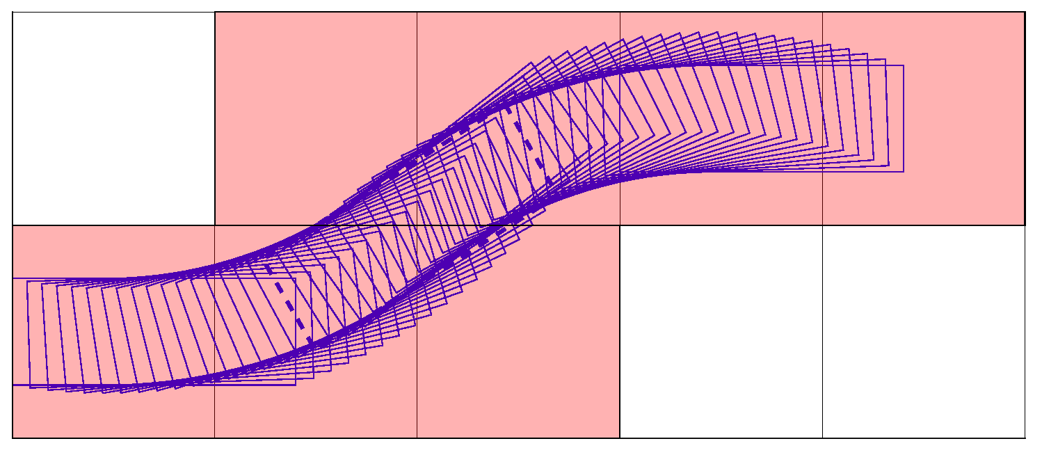
Similar to turning actions, a typical lane-changing maneuver is also modeled and outlined in Figure 9. The forklift goes forward and changes to the left lane, which is shown on the top row in Figure 9. The other possible node-expanding paths of turning and lane changing are modeled by mirroring or rotating the examples reported in Figs. 8 and 9.
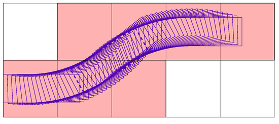
Figure 9.
Path of lane changing.
The smoothness of the modeled paths can be enhanced by adopting advanced techniques, and the identical heuristic trajectory search rule of this work can also be applied to the newly modeled paths.
4.2. Velocity Planner
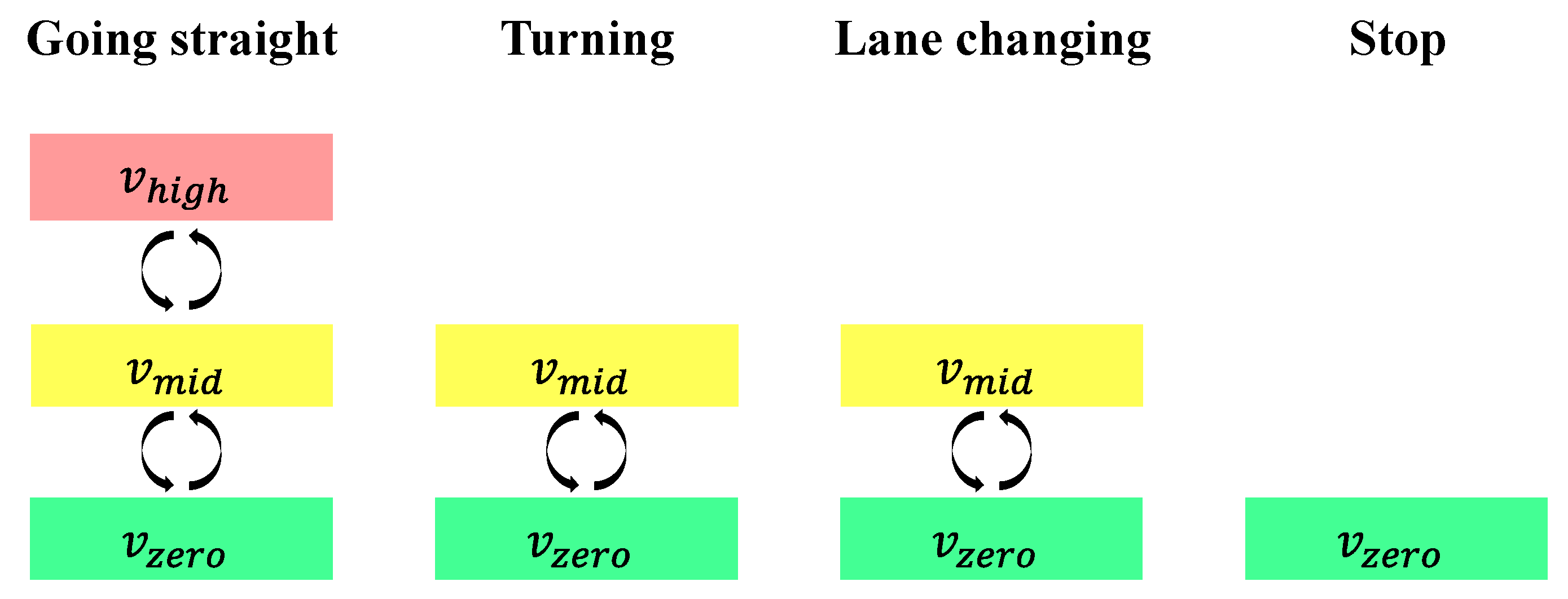
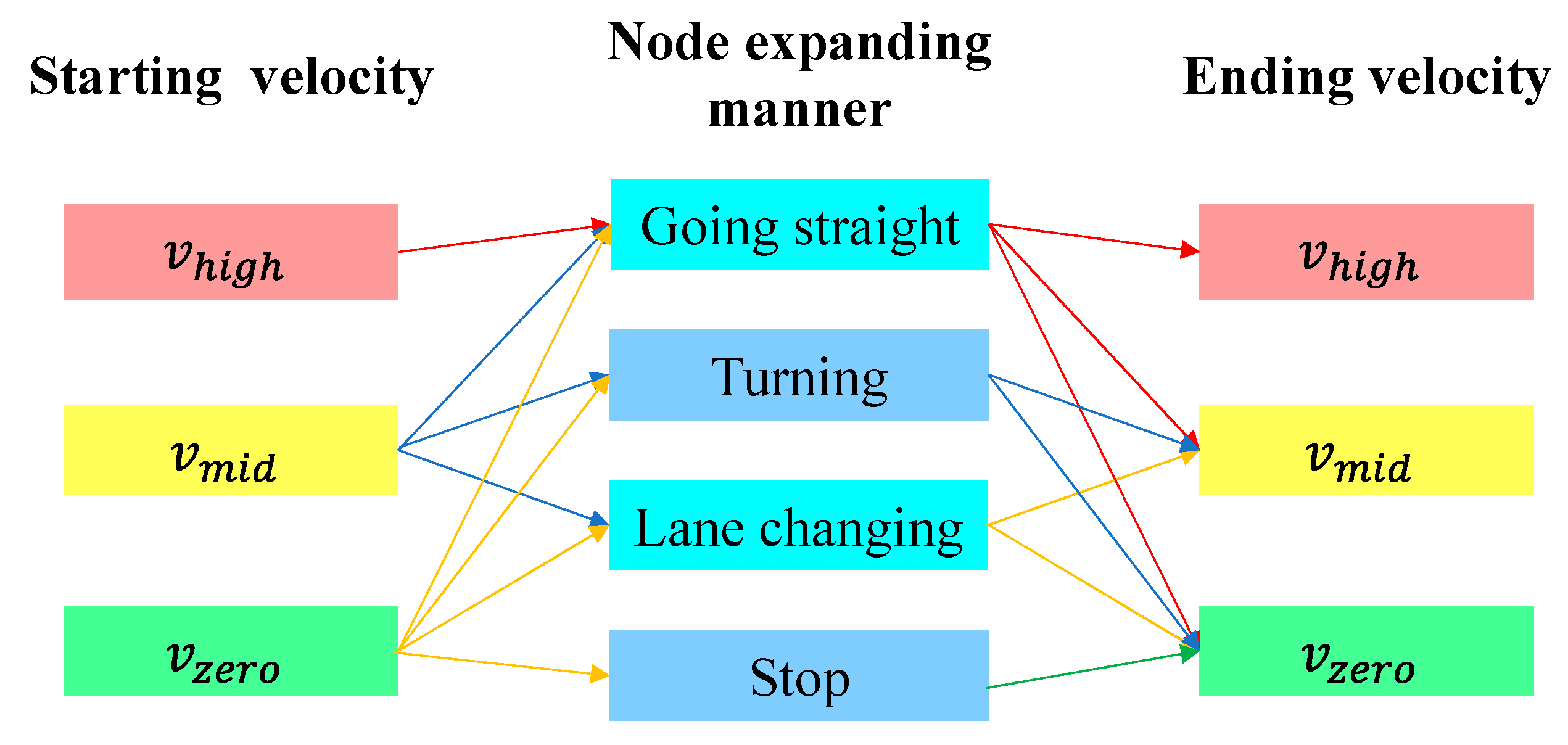
The velocity planner determines the node expansion rule in the time domain and the potential node arrival instants. When one maneuver starts or finishes, the vehicle speed solely falls into one of three determined constants (, and ), which correspond to high speed, mid speed, and zero speed. Figure 10 reports all possible velocity selections linked to the start and end of the maneuvers. can only be selected with the expansion pattern of going straight to fulfill the kinematic constraints given by Equations (1) and (2). The stop maneuver is an expansion of finite value solely on the time domain, it follows that only can be applied to this action.
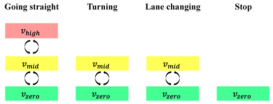
Figure 10.
Velocity selections when one maneuver starts or ends.
The velocity level over one maneuver can only be linked to itself or an adjacent one, although all maneuvers can be arbitrarily linked along a trajectory. In other words, during one maneuver, the vehicle speed can maintain or alter among those three velocities, but the direct change between and is illegal. For instance, if the vehicle finishes a series of going straight actions with speed , its ending velocity of the last second action should then be or . Likewise, if turning follows going straight with an original velocity , the speed of the last going straight maneuver should reduce to to gain an initial velocity for turning.
Following the velocity selection rules, all possible speed variations through one maneuver are shown in Figure 11. It is noteworthy that the link of →Going straight→ and the opposite link are infeasible. Thus, 16 connection choices in total are applicable. Furthermore, velocity is merely an intermediate state used to determine a time dimension expansion, although it is a vital parameter for motion planning. The detailed velocity time history during one maneuver can be modeled by applying varied techniques to obtain the required initial and finishing speeds. In the current work, deceleration or acceleration along one action between the same velocity levels is modeled with identical time lengths, with the aim of simple calculation. The number of time expansion selections (cf. with in Table 1) thus reduces to 12.
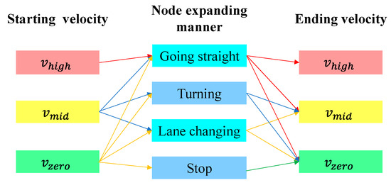
Figure 11.
Velocity variations through one maneuver.

Table 1.
Node expansion selections in time domain.
The function determines time expansion data based on Table 2, which is elaborated as follows. When planning a trajectory, the maximum feasible velocities are consistently selected for all maneuvers with zero speed supplied to the start and end of the trajectory. With regard to one node expansion, three values of , and are initially saved in the parent node as the possible start instant of the maneuver, and these respectively correspond to ending velocities of , , and , if they exist. In the cases where is not reachable, the value stored in will be the minimum time length during the maneuver, with ending velocity . Consequently, . Similar result of is obtained when the maximum realizable ending velocity is . As the parent node is initialized, values of , , and are derived and saved for the child node with the identical manner for the parent node. Furthermore, the starting velocity of a new expansion may be imposed as , combined with the node expansion type of the previous maneuver. A stopping flag is then set as 1. Such a case happens when an expansion of stop occurs or moving direction of a vehicle is reversed. In the rest of the working conditions, the flag remains 0. Notably, a node is of four dimensions, , , , and ; among them, is an index used in the graph search, and more than one value stored in one index could complicate the problem. Consequently, only the -related time instant is stored as the node index.

Table 2.
Model-based approach for saving time consumption data.
Meanwhile, each node stores three ending time instants. Thus, one algorithm should be applied to select the exact ending instant of each node. This algorithm first chooses the minimum time of each maneuver over the path. The deceleration phase is then imposed on the last two nodes of the trajectory, and the corresponding and are in turn assigned to these two nodes as the maneuver-finishing time instants. As the above methods are implemented from the start to the end of the initialized trajectory, a few modifications are imposed to fix the node time indices in certain circumstances. For instance, when , the maximum achievable ending time for the former maneuver node is determined by selecting the value of . In this case, the ending velocity of this maneuver turns to be . Meanwhile, in the same combination of maneuvers, if a previous maneuver exists and , is assigned to , as the prior maneuver cannot achieve a higher velocity.
4.3. Collision Detection Strategy
The pseudocode of the collision detection function is recorded in Algorithm 3. A variable is used as a flag to indicate the validity of the node expansion as well as the type of collisions that may have occurred. When the current expansion is valid, is set as 0. means that at least the ending pose of the expansion risks colliding, and signifies that the invalidity is only found in the link between the starting and final locations. This algorithm consists of two parts, which separately refer to collisions that occurred with ending and intermediate pose of the vehicle. As regards both circumstances, collisions should be avoided throughout .
| Algorithm 3: Collision detection algorithm |
|
Static obstacles correspond to the walls of the shelves and warehouse, and the related collision detection method is expressed on lines 4 to 7 in Algorithm 3. is used to obtain the current pose based on the parent pose and the current expansion manner . The function is applied to check if collisions with static obstacles exist. This check is first judged by identifying the validity of the final pose. When it comes to maneuvers of turning and lane changing, an additional intermediate pose (cf. thick dashed rectangular in Figure 8 and Figure 9), obtained through , should be further examined (cf. lines 15 to 18 in Algorithm 3). Focusing on the collision avoidance constraints formulation between the point ( and denotes the obstacle point number) and the current investigated vehicle featuring vertexes , , and . A collision forms when enters the rectangle . The restriction that is located outside of the rectangle can be formulated by applying a triangle-area-based criterion [38],
where indicates the triangle area, and refers to the rectangle area. Applying Equation (11) to every node expansion with respect to every obstacle point, the static obstacle collision judgement is yielded.
Dynamic obstacles in the current study are only forklifts, whose motions have been saved in , and the function is applied to find in and by calling Table 2. As reported in Figure 8 and Figure 9, the highlighted grids indicate the approximate area occupied during the movements of turning and lane changing. Similarly, the covered grids pertaining to other maneuvers in the same category can be determined by mirroring or rotating the highlighted grids (cf. Figure 8 and Figure 9). The functions and are respectively used to record the covered grids of the final pose and the intermediate pose for the current node expansion patterns.
Without loss of generality, let us focus on the collision avoidance constraint formulation between the vehicle and the vehicle ( and ). The function is first utilized to search for the covered grids by the vehicles , whose trajectories are not being planned, with respect to time. It is possible that no actions of the forklift have been determined during the period when the current maneuver of vehicle could occupy. Under such circumstances, the grids that the vehicle finally parks are treated as the covered ones.
Finally, is used to detect if or is going to simultaneously cover the grids already stored in over the valid time. Notably, during the collision detection, the current action is virtually regarded as the final maneuver with set as the finishing velocity with selected, thus an equal or longer time length of this maneuver in actual operation is considered. This treatment can enhance the safety performance to certain extents.
Notably, referring to Algorithm 3, the types of failure through an expansion have been noticed when one expansion has failed. This provides a tool to distinguish if one child node should be closed or skipped because that failure can be simply due to the intermediate trajectory of the action is interfered, while the corresponding child node could be valid in other situations.
4.4. Trajectory Cost Function
The function is explained in this section. With regard to one node expansion, the cost function is the sum of two parts, as reported in Equation (12),
in which stands for the cumulative cost from the initial pose to the current pose and indicates the estimated cost from the child node of the current expansion to the target node of the trajectory being defined. is a calibrated weighting aimed at achieving a balance between the computational resources used for searching and the resultant trajectory’s quality. In total, it is expected that one forklift complete a delivery or return subtasks subjected to the minimum travelling time of . Meanwhile, times of turning, lane changing, and speed inverse maneuvers should be minimized in order to reduce unnecessary movements, which may decrease the traffic capacity of the passages.
As far as the function of trajectory to the goal is concerned, Equation (13) is applied. We used the Manhattan distance plus another function of . Both the distance and the angle are evaluated in times of certain characteristic dimensions.
where , indicating the grid side length; , , and correspond to the goal space coordinates; , , and refer to the coordinates of the current expansion child node.
The passed trajectory cost function that characterizes the time consumed from the starting pose of the trajectory to the current one writes:
where , , and respectively indicate the predefined penalties pertaining to single time of turning, lane changing, and speed inverse. , , and denote the cumulative number of corresponding maneuvers from the initial pose to the current child node along the trajectory being defined.
In addition, if one node originally stored in is reached a second time with a reduced value of during a node expansion compared to the previous saved for the same nodes, the function is used to switch the parent node to the parent node of current expansion, with the aim of reducing calculation time length and optimizing the trajectory being planned.
5. Joint Dispatching and Cooperative Trajectory Planning Framework
The trajectories of forklift vehicles in the warehouse are sequentially determined in the complete cooperative operative algorithm (cf. Algorithm 4). Generally, the dispatching technique is first applied to select the current vehicle index as well as the goal coordinate in the space domain for the current trajectory planning subtask. Subsequently, an improved hybrid A* search algorithm is used to determine all details pertaining to the newly planned trajectory . The above methods are repeated until all stack locations in the warehouse are filled, as the warehouse filling state is being updated.
The function is used to derive the number of unfilled stacks. The function is then applied to find the parent node for the next expansion with minimum cost found in and to simultaneously remove this node from .
A maximum number of iterations in the improved hybrid A* algorithm is induced to break the endless iterations that may derive a trajectory involving an unacceptable waiting period. The improved hybrid A* search algorithm is finished by satisfying any one of the three criteria, which are, respectively, the goal coordinate reached as a new child node, the iteration number exceeding , and no node saved in . Among them, only the first criterion indicates the trajectory of the current subtask is successfully planned, and a corresponding flag is thus set as 1 to declare this success.
The function is employed to generate the trajectory with the newly planned trajectory by backtracking from to with as the ending instants. During the backtracking, the maximum realizable velocities of the intermediate nodes are selected based on the manner depicted in Figure 11 and Table 2.
Finally, the function updates as the stack located at has been filled.
| Algorithm 4: Cooperative operation algorithm |
|
6. Numerical Experiments
Simulations of filling and emptying missions were conducted on the MATLAB 2021b platform, utilizing the parametric settings reported in Table 3. Each warehouse filling or emptying mission began with fully empty or filled initial conditions, respectively. The motion planning for each forklift in the simulation environment solely takes into account obstacles such as warehouse walls and other forklifts.

Table 3.
Parametric settings regarding model and approach.
The simulation results are divided into two parts. The first part focuses on assessing the consistency of the motion planning strategy by presenting three short-time trajectories for multiple forklifts. In the second part, various dispatching strategies were benchmarked using different scores specifically designed for the current warehouse scenario. This evaluation was conducted to determine the performance and efficiency of different dispatching strategies in the given warehouse scenario.
6.1. On the Performance of the Trajectory Planning Technique
Figure 12 reports how forklift 1 returns to a picking station from shelf cluster , where it has just unloaded goods. Before the start of the scenario, forklifts 2 and 4 are in the same state of return, and forklift 3 is unloading in shelf cluster . When the scene in Figure 12 starts, forklift 1 accelerates and decelerates to reverse to the entrance of shelf cluster . At the meantime, forklift 4 turns and heads to the picking station , leaving the crossing of the wide passages empty. With the purple square showing the newly filled stack, forklift 3 leaves shelf cluster and enters to finish turning round. When it is inside of , forklift 1 goes through the passage between and . Subsequently, forklift 1 reverses and turns to the picking station , and forklift 3 then enters the wide passages to return to the assigned picking station, which is . Finally, forklift 2 is the first vehicle that arrives at the crossing area of wide passages with the goods picked. During the scenario, all trajectories are directly determined by means of the approach elaborated on in Section 4. The least priority is dynamically offered to the newly departed vehicle. For instance, in this scenario, forklift 3 initially has the lowest priority. Thus, it should judge if there is enough time for the vehicle to turn around. Therefore, if the time is limited, vehicle 3 would wait at the entrance of , until the passing of forklift 1.
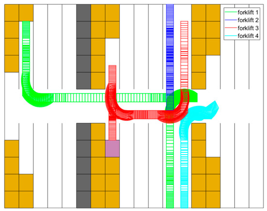
Figure 12.
Planned trajectories between s and s.
Figure 13 shows how the last stack is filled. Because there is nowhere to be filled hereafter, forklift 3 is parked in one picking station, and forklift 1 heads to picking station and stops. Initially, forklift 4 has just finished one unloading process, then it enters shelf cluster to turn over. After forklift 4 leaves , forklift 2 enters the shelf cluster to complete the last delivery subtask. Meanwhile, forklift 4 accelerates, decelerates, and turns to picking station for final parking.
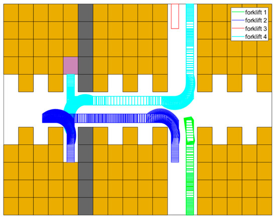
Figure 13.
Planned trajectories between s and s.
Figure 14 shows a scenario where the trajectory decision for forklift 3 encounters a failure. In this case, forklift 1 reaches shelf to unload goods, while forklift 3 completes its unloading process earlier than forklift 1. Consequently, forklift 3 should be assigned a higher priority to plan the trajectory based on function . However, at this moment, forklift 1 remains stationed at the entrance of shelf , obstructing the passage for forklift 3. As a result, a decision failure occurs, leading to an update in the trajectory planning priority stored in . Only after the completion of the trajectory planning for forklift 1 can the trajectory planning for forklift 3 proceed accordingly.
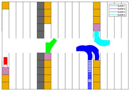
Figure 14.
Planned trajectories between s and s.
6.2. On the Performance of Dispatching Strategies
Table 4 benchmarks five distinct dispatching strategies for both filling and emptying tasks. It is worth noting that these dispatching methods are applicable only to specific coupling scenarios between grids and vehicle maneuvers, as they incorporate a preliminary A* search during the dispatching process.

Table 4.
Benchmark of the different dispatching strategies.
The approaches differ in the assignment methods pertaining to delivering subtasks. While the decision failure times in Table 4 indicate the number of times or is changed without a solid trajectory decided throughout the entire warehouse filling mission, the end time is the finishing timing of the same task. Among the strategies, ANN combined determines the goal through (cf. in Equation (9)) when the coefficients of the MLP are determined. Comprehensive strategy applies in Equation (3), and the target is determined based on . The other three strategies only concern a few parameters in Equation (3). Greedy, traffic jam removal, and balance strategies select the goal pose through , and respectively.
As reported in Table 4, the end time of the emptying task is approximately 10% longer than that for filling tasks. However, the occurrence of decision failure times is generally lower. This indicates that during emptying tasks, instances of a forklift obstructing routes and blocking other vehicles for extended periods are rare. Yet, with the current configuration of and , all vehicles might experience longer wait times on average during each subtask.
The ANN combined strategy is the optimal method in terms of end time for both filling and emptying tasks, requiring approximately 2% less time than the comprehensive strategy. However, it does exhibit comparable or even slightly greater decision failure times when compared to the comprehensive strategy. In general, a reduction in the first parameter can reduce the computation burden of the hardware by performing fewer useless calculations in searching a trajectory. The second parameter directly shows the efficiency of the cooperative operation of multiple forklifts. Notably, the ANN approach applied to train the dispatching system only concerns the efficiency of planning a trajectory for the current vehicle. Therefore, it is possible that some stacks in only one shelf cluster are left to be filled by selecting the best solution multiple times. In this case, multiple forklifts have to cooperatively fill one shelf cluster, and the waiting period of each vehicle must increase. Therefore, both the decision failure times and the end time may sharply increase.
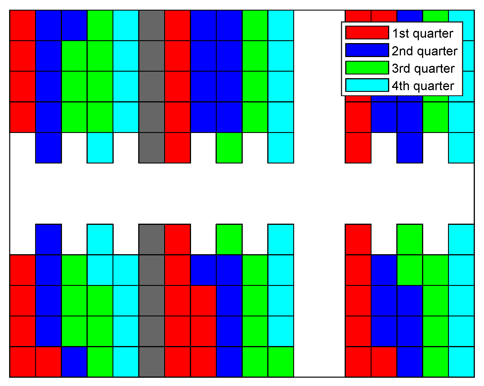
In Figure 15, Figure 16, Figure 17 and Figure 18, the sequence in which the warehouse is filled with different methods is reported. The colored blocks plotted in the schematic warehouse stand for the stacks filled during different periods (red for the first quarter of time, blue for the second, green for the third, and cyan for the last). It is observed that the filling of different shelf clusters for the ANN combined strategy (cf. Figure 15) in different quarters of the period is balanced to a certain extent. There are, respectively, 35, 37, 34, and 30 stacks filled during each quarter. Particularly in the last quarter of the period, similar numbers of stacks filled are distributed within all six shelf clusters, and this provides a possibility for a feasible and fast solution to filling the warehouse.
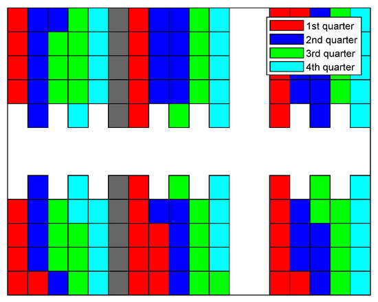
Figure 15.
Filling sequence of ANN combined strategy.
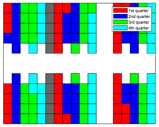
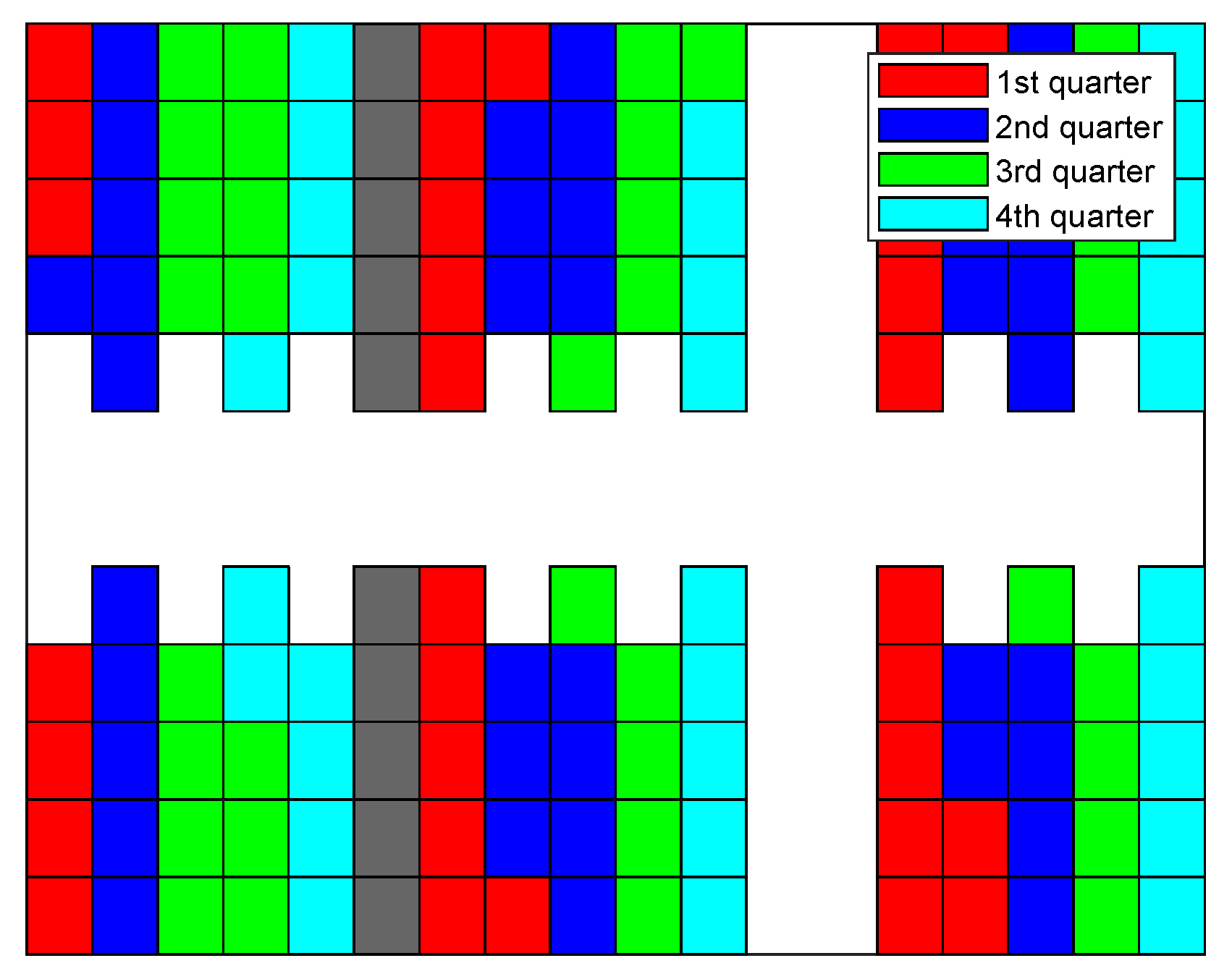
Figure 16.
Filling sequence of comprehensive strategy.
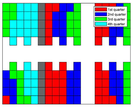
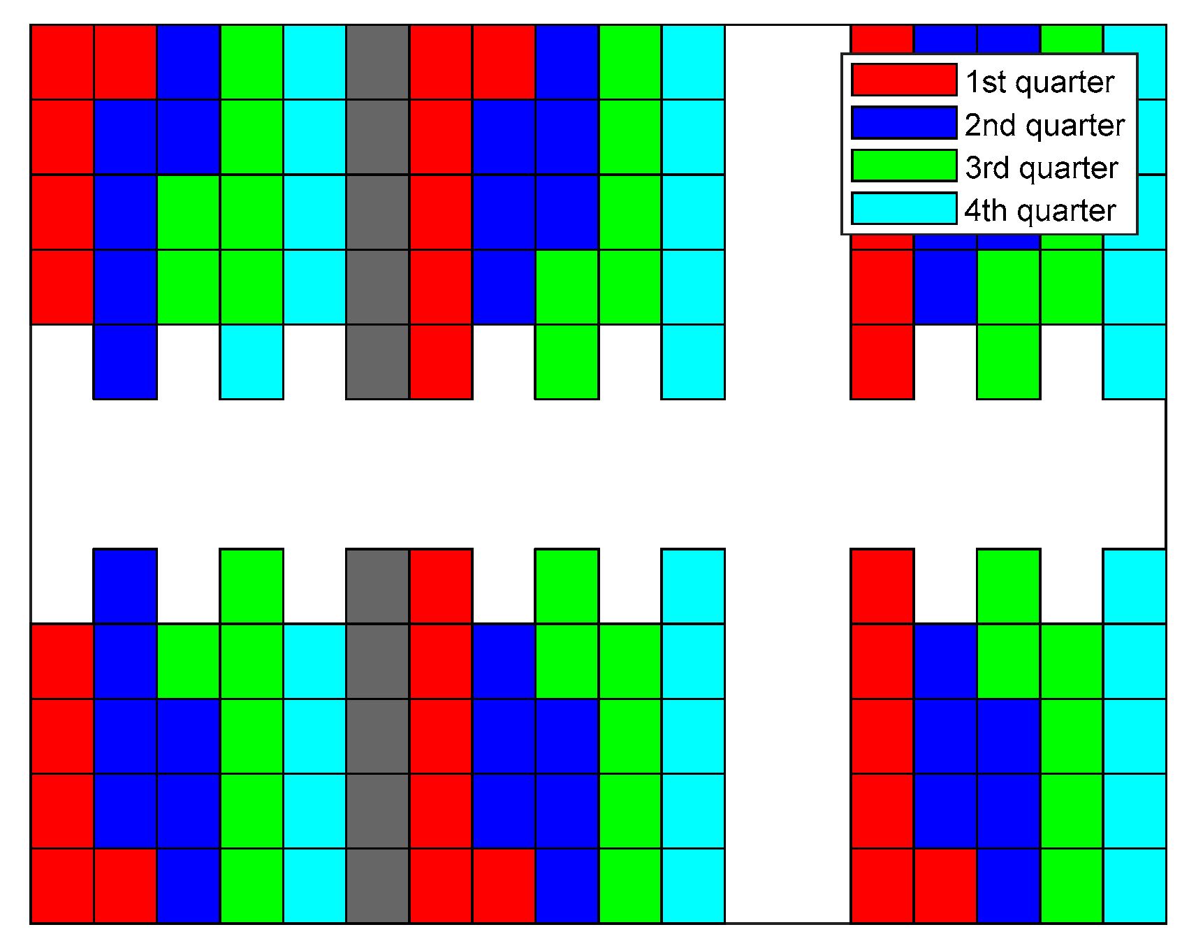
Figure 17.
Filling sequence of traffic jam removing strategy.
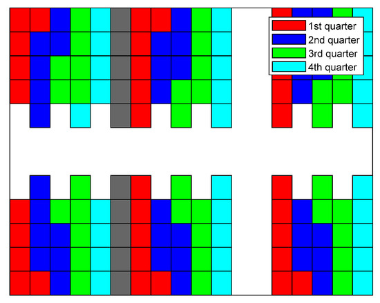
Figure 18.
Filling sequence of balance strategy.
By excluding the MLP of ANN, a comprehensive strategy is also capable of assigning subtasks to each forklift explicitly. Although the performance is slightly worse than the ANN combined one, it does not require the data pertaining to previous cycles. Figure 16 demonstrates the filling sequence for this approach. Similar to that of the ANN combined approach, the filling state of the shelf clusters in the warehouse is relatively balanced throughout the period. A few seconds are added in terms of the end time for this strategy without the fine adjustment of the MLP.
Figure 17 exhibits the filling sequence of the traffic-jam-removing strategy. The difference between this method and the greedy strategy is that the previous one simultaneously considers in Equation (3). One stack in shelf cluster is filled in the first quarter of the period, and both the decision failure times and the end time pertaining to the traffic jam removal approach reduce compared to the greedy strategy. Thus, a simple additional function of can slightly further characterize the difficulty of the trajectory planning. Meanwhile, because the filling sequences of these two strategies are similar, the figure pertaining to the greedy method is omitted. As shown in Figure 17, it basically evenly fills shelf clusters , , and in the first quarter of the period. The majority of stacks in and around a third of stacks in are filled in the last quarter. Considering four vehicles cooperatively delivering goods, violations between trajectories evidently arise, and the times of failure in trajectory decisions and the waiting time can increase markedly.
The filling sequence of the balance strategy is plotted in Figure 18. The filling of different shelf clusters is nearly perfectly balanced. Evidently, this strategy can better arrange the trajectories to fill the last few stacks of the warehouse compared to any other approach. Therefore, the number of stacks filled during the last quarter of the warehouse filling cycle is comparable to that during other periods. In particular, when the 5th, 14th, and 23rd stacks of shelf clusters and (cf. Figure 2) are being filled, the paths between the shelf clusters ( and ) in the left side of the warehouse (cf. Figure 1) and picking stations are cut. Meanwhile, the first delivery vehicle reaching these certain stack locations between shelf clusters and can simultaneously block the routes to certain shelf clusters. This phenomenon also appears in shelf clusters and when the identical stack indexes are considered. Those are the unique conflicts that arose to cause the failure decisions and the lengthening of the end time for the balance strategy.
7. Conclusions
This study presents a joint dispatching and cooperative trajectory planning framework. In this framework, the dispatching method applies a time dimension involved A* search, which is used to score different goal poses during a delivery subtask. ANN is simultaneously implemented to evaluate the difficulties for a forklift to arrive at a goods unloading pose from a picking station. In addition, the stacks to be filled pertaining to different shelf clusters are used as the third parameter to balance the shelf filling states, with the aim of avoiding deadlocks at the final stage of the mission.
As far as the trajectory planning approach within the framework is concerned, a model-based improved A* search algorithm is used to sequentially determine the trajectory of each vehicle without further optimization-based techniques. The node expansion manners are determined on the basis of the purpose of a maneuver, and the speed pertaining to the start and end of a maneuver is divided into stages.
Different dispatching strategies are benchmarked. The ANN combined strategy shows the best performance in warehouse filling efficiency, but the decision failure times of this method are comparable to those of the comprehensive strategy. Meanwhile, it is observed that the balance of the filling state pertaining to shelf clusters is as important as the evaluation of the goal-reaching difficulties. Furthermore, the trajectories of multiple vehicles in a short time are presented. It is shown that although the priority of a vehicle during one subtask is predefined, the vehicles are capable of cooperatively and continuously finding feasible trajectories.
In the future, our joint strategy will be tested in a downsized unmanned warehouse setup. Additionally, we aim to implement a zonal shutdown feature for enhanced safety in case pedestrians enter the area. We also plan to integrate a forklift failure detection mechanism to enable uninterrupted warehouse operations even in the presence of a few malfunctioning forklifts.
Author Contributions
Conceptualization, T.Z., M.L. and K.C.; methodology, H.L. and Y.F.; validation, T.Z., Y.F. and K.C. All authors have read and agreed to the published version of the manuscript.
Funding
This research was funded by Fundamental Research Funds for the Central Universities: 531118010692; National Natural Science Foundation of China: 62103139; Fundamental Research Funds for the Central Universities: 531118010509; Natural Science Foundation of Hunan Province, China: 2021JJ40114.
Conflicts of Interest
The authors declare no conflict of interest.
References
- Bozek, P.; Karavaev, Y.L.; Ardentov, A.A.; Yefremov, K.S. Neural network control of a wheeled mobile robot based on optimal trajectories. Int. J. Adv. Robot. Syst. 2020, 17, 2. [Google Scholar] [CrossRef]
- Blatnický, M.; Dižo, J.; Sága, M.; Gerlici, J.; Kuba, E. Design of a Mechanical Part of an Automated Platform for Oblique Manipulation. Appl. Sci. 2020, 10, 8467. [Google Scholar] [CrossRef]
- Yang, Q.; Lian, Y.; Xie, W. Hierarchical planning for multiple AGVs in warehouse based on global vision. Simul. Model. Pract. Theory 2020, 104, 102124. [Google Scholar] [CrossRef]
- Li, G.; Wang, X.; Yang, J.; Wang, B. A new method to design fuzzy controller for unmanned autonomous forklift. In Proceedings of the 2015 IEEE International Conference on Robotics and Biomimetics (ROBIO), Zhuhai, China, 6–9 December 2015; pp. 946–951. [Google Scholar] [CrossRef]
- Zhong, Z.; Wan, M.; Pei, Z.; Qin, X. Spatial and temporal optimization for smart warehouses with fast turnover. Comput. Oper. Res. 2021, 125, 105091. [Google Scholar] [CrossRef]
- Weidinger, F.; Boysen, N.; Briskorn, D. Storage assignment with rack moving mobile robots in KIVA warehouses. Transp. Sci. 2018, 52, 1297–1588. [Google Scholar] [CrossRef]
- Yu, W.; Wang, S.; Wang, R.; Tan, M. Generation of temporal-spatial Bezier curve for simultaneous arrival of multiple unmanned vehicles. Inf. Sci. 2017, 418–419, 34–45. [Google Scholar] [CrossRef]
- Ouyang, Y.; Li, B.; Zhang, Y.; Acarman, T.; Guo, Y.; Zhang, T. Fast and optimal trajectory planning for multiple vehicles in a nonconvex and cluttered environment: Benchmarks, methodology, and experiments. In Proceedings of the 2022 IEEE International Conference on Robotics and Automation (ICRA), Philadelphia, PA, USA, 23–27 May 2022; pp. 10746–10752. [Google Scholar]
- Chen, B.M. On the trends of autonomous unmanned systems research. Engineering 2022, 12, 20–23. [Google Scholar] [CrossRef]
- Miyamoto, T.; Inoue, K. Local and random searches for dispatch and conflict-free routing problem of capacitated AGV systems. Comput. Ind. Eng. 2016, 91, 1–9. [Google Scholar] [CrossRef]
- Stutzle, T.; Ruiz, R. Iterated Local Search. In Handbook of Heuristics; Marti, R., Pardalos, P., Resende, M., Eds.; Springer: Cham, Switzerland, 2018. [Google Scholar] [CrossRef]
- Zhang, X.; Sang, H.; Li, J.; Han, Y.; Duan, P. An effective multi-AGVs dispatching method applied to matrix manufacturing workshop. Comput. Ind. Eng. 2022, 163, 107791. [Google Scholar] [CrossRef]
- Lin, L.; Shinn, S.W.; Gen, M.; Hwang, H. Network model and effective evolutionary approach for AGV dispatching in manufacturing system. J. Intell. Manuf. 2006, 17, 465–477. [Google Scholar] [CrossRef]
- Bao, Y.; Jiao, G.; Huang, M. Cooperative optimization of pod repositioning and AGV task allocation in Robotic Mobile Fulfillment Systems. In Proceedings of the 2021 33rd Chinese Control and Decision Conference (CCDC), Kunming, China, 22–24 May 2021; pp. 2597–2601. [Google Scholar] [CrossRef]
- Lee, I.G.; Chung, S.H.; Yoon, S.W. Two-stage storage assignment to minimize travel time and congestion for warehouse order picking operations. Comput. Ind. Eng. 2020, 139, 106129. [Google Scholar] [CrossRef]
- Fragapane, G.; de Koster, R.; Sgarbossa, F.; Strandhagen, J.O. Planning and control of autonomous mobile robots for intralogistics: Literature review and research agenda. Eur. J. Oper. Res. 2021, 294, 405–426. [Google Scholar] [CrossRef]
- Hu, H.; Jia, X.; He, Q.; Fu, S.; Liu, K. Deep reinforcement learning based AGVs real-time scheduling with mixed rule for flexible shop floor in industry 4.0. Comput. Ind. Eng. 2020, 149, 106749. [Google Scholar] [CrossRef]
- Zhou, T.; Tang, D.; Zhu, H.; Zhang, Z. Multi-agent reinforcement learning for online scheduling in smart factories. Robot. Comput.-Integr. Manuf. 2021, 72, 102202. [Google Scholar] [CrossRef]
- Lian, Y.; Yang, Q.; Liu, Y.; Xie, W. A spatio-temporal constrained hierarchical scheduling strategy for multiple warehouse mobile robots under industrial cyber-physical system. Adv. Eng. Inform. 2022, 52, 101572. [Google Scholar] [CrossRef]
- Liu, Y.; Du, Y.; Dou, S.; Peng, L.; Su, X. Research summary of intelligent optimization algorithm for warehouse AGV path planning. In Lecture Notes in Operations Research; Shi, X., Bohács, G., Ma, Y., Gong, D., Shang, X., Eds.; Springer: Singapore, 2022. [Google Scholar] [CrossRef]
- Ma, Y.; Wang, H.; Xie, Y.; Guo, M. Path planning for multiple mobile robots under double-warehouse. Inf. Sci. 2014, 278, 357–379. [Google Scholar] [CrossRef]
- Xidias, E.K. A decision algorithm for motion planning of car-like robots in dynamic environments. Cybern. Syst. 2021, 52, 1909844. [Google Scholar] [CrossRef]
- Li, B.; Acarman, T.; Zhang, Y.; Ouyang, Y.; Yaman, C.; Kong, Q.; Zhong, X.; Peng, X. Optimization-based trajectory planning for autonomous parking with irregularly placed obstacles: A lightweight iterative framework. IEEE Trans. Intell. Transp. Syst. 2022, 23, 11970–11981. [Google Scholar] [CrossRef]
- Li, B.; Zhang, Y.; Feng, Y.; Zhang, Y.; Ge, Y.; Shao, Z. Balancing computation speed and quality: A decentralized motion planning method for cooperative lane changes of connected and automated vehicles. IEEE Trans. Intell. Veh. 2018, 3, 340–350. [Google Scholar] [CrossRef]
- Zhou, Y.; Huang, N. Airport AGV path optimization model based on ant colony algorithm to optimize Dijkstra algorithm in urban systems. Sustain. Comput. Inform. Syst. 2022, 35, 100716. [Google Scholar] [CrossRef]
- Zacharia, P.T.; Xidias, E.K. AGV routing and motion planning in a flexible manufacturing system using a fuzzy-based genetic algorithm. Int. J. Adv. Manuf. Technol. 2020, 109, 1801–1813. [Google Scholar] [CrossRef]
- Kneissl, M.; Madhusudhanan, A.K.; Molin, A.; Esen, H.; Hirche, S. A multi-vehicle control framework with application to automated valet parking. IEEE Trans. Intell. Transp. Syst. 2021, 22, 5697–5707. [Google Scholar] [CrossRef]
- Dresner, K.; Stone, P. Multiagent traffic management: A reservation-based intersection control mechanism. In Proceedings of the Third International Joint Conference on Autonomous Agents and Multiagent Systems, New York, NY, USA, 23 July 2004; pp. 530–537. [Google Scholar]
- Guney, M.A.; Raptis, I.A. Dynamic prioritized motion coordination of multi-AGV systems. Robot. Auton. Syst. 2021, 139, 103534. [Google Scholar] [CrossRef]
- Digani, V.; Caramaschi, F.; Sabattini, L.; Secchi, C.; Fantuzzi, C. Obstacle avoidance for industrial AGVs. In Proceedings of the 2014 IEEE 10th International Conference on Intelligent Computer Communication and Processing (ICCP), Cluj-Napoca, Romania, 4–6 September 2014; pp. 227–232. [Google Scholar] [CrossRef]
- Stern, R. Multi-Agent Path Finding—An Overview. In Artificial Intelligence. Lecture Notes in Computer Science; Osipov, G., Panov, A., Yakovlev, K., Eds.; Springer: Cham, Switzerland, 2019; Volume 11866. [Google Scholar] [CrossRef]
- Zhang, J.; Li, Z.; Li, L.; Li, Y.; Dong, H. A bi-level cooperative operation approach for AGV based automated valet parking. Transp. Res. Part C 2021, 128, 103140. [Google Scholar] [CrossRef]
- Meng, Y.; Li, L.; Wang, F.; Li, K.; Li, Z. Analysis of cooperative driving strategies for nonsignalized intersections. IEEE Trans. Veh. Technol. 2018, 67, 2900–2911. [Google Scholar] [CrossRef]
- Lee, C.K.M.; Lin, B.; Ng, K.K.H.; Lv, Y.; Tai, W.C. Smart robotic mobile fulfillment system with dynamic conflict-free strategies considering cyber-physical integration. Adv. Eng. Inform. 2019, 42, 100998. [Google Scholar] [CrossRef]
- Rochel, P.; Rios, H.; Mera, M.; Dzul, A. Trajectory tracking for uncertain Unicycle Mobile Robots: A Super-Twisting approach. Control Eng. Pract. 2022, 122, 105078. [Google Scholar] [CrossRef]
- Zhang, T. An estimation method of the fuel mass injected in large injections in Common-Rail diesel engines based on system identification using artificial neural network. Fuel 2022, 310, 122404. [Google Scholar] [CrossRef]
- Dolgov, D.; Thrun, S.; Montemerlo, M.; Diebel, J. Path planning for autonomous vehicles in unknown semi-structured environment. Int. J. Robot. Res. 2010, 29, 485–501. [Google Scholar] [CrossRef]
- Li, B.; Shao, Z. A unified motion planning method for parking an autonomous vehicle in the presence of irregularly placed obstacles. Knowl. Based Syst. 2015, 86, 11–20. [Google Scholar] [CrossRef]
Disclaimer/Publisher’s Note: The statements, opinions and data contained in all publications are solely those of the individual author(s) and contributor(s) and not of MDPI and/or the editor(s). MDPI and/or the editor(s) disclaim responsibility for any injury to people or property resulting from any ideas, methods, instructions or products referred to in the content. |
© 2023 by the authors. Licensee MDPI, Basel, Switzerland. This article is an open access article distributed under the terms and conditions of the Creative Commons Attribution (CC BY) license (https://creativecommons.org/licenses/by/4.0/).

